Proximity Drawings of High-Degree Trees

Abstract.

A drawing of a given (abstract) tree that is a minimum spanning tree of the vertex set is considered aesthetically pleasing. However, such a drawing can only exist if the tree has maximum degree at most 6. What can be said for trees of higher degree? We approach this question by supposing that a partition or covering of the tree by subtrees of bounded degree is given. Then we show that if the partition or covering satisfies some natural properties, then there is a drawing of the entire tree such that each of the given subtrees is drawn as a minimum spanning tree of its vertex set.

1. Introduction

The field of graph drawing studies aesthetically pleasing drawings of graphs. There are a number of recognised criteria for measuring the quality of a drawing of a given graph. These include:

• no two edges should cross in drawings of planar graphs;

• the edges should be drawn as straight line-segments; and

• the drawing should have large angular resolution (defined to be the minimum angle determined by two consecutive edges incident to a vertex).

These three criteria are adopted in the present paper. More formally, a (straight-line general position) drawing of graph $G$ is an injective function $\phi:V(G)\rightarrow\mathbb{R}^{2}$ such that the points $\phi(u),\phi(v),\phi(w)$ are not collinear for all distinct vertices $u,v,w\in V(G)$. The image of an edge $vw\in E(G)$ under $\phi$ is the line segment $\overline{\phi(v)\phi(w)}$. Where no confusion is caused, we henceforth do not distinguish between a graph element and its image in a drawing. Two edges cross if they intersect at a point other than a common endpoint.

Our focus is on drawings of trees. Here a number of other criteria have been studied that will not be considered in this paper. These include: small bounding box area [9, 7, 27, 33, 8, 23, 11], small aspect ratio [23, 8], few bends in the edges [28], few distinct edge-slopes [14], few distinct edge-lengths [6], layered vertices [34], upwardness in rooted trees [36, 11, 28, 7], and maximising symmetry [24].

A minimum spanning tree of a finite set $P\subset\mathbb{R}^{2}$, denoted by ${\sf MST}(P)$, is a straight-line drawing of a tree with vertex set $P$ and with minimum total edge length; see Figure 1 for an example. A drawing of a given (abstract) tree that is a minimum spanning tree of its vertex set is considered to be particularly aesthetically pleasing. In particular, every minimum spanning tree is crossing-free and has angular resolution at least $\frac{\pi}{3}$. Drawings defined in this way are called ‘proximity drawings’; see Section 2 and [1, 2, 32, 31, 4, 12, 30] for more on proximity drawings.

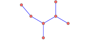
Figure 1. Example of a minimum spanning tree.

Monma and Suri [31] proved that every degree-$5$ tree can be drawn as a minimum spanning tree of its vertex set, and they provided a linear time (real RAM) algorithm to compute the drawing. In any drawing of a vertex $v$ with degree at least $7$, some angle at $v$ is greater than $\frac{\pi}{3}$, and the same is true for a degree-$6$ vertex if the points are required to be in general position. Thus a tree that contains a vertex with degree at least $7$ cannot be drawn as a minimum spanning tree, and the same is true for a degree-$6$ vertex if the points are in general position. If collinear vertices are allowed, then Eades and Whitesides [18] showed that it is NP-hard to decide whether a given degree-$6$ tree can be drawn as a minimum spanning tree. In this sense, the problem of testing whether a tree can be drawn as a minimum spanning tree is essentially solved. (In related work, Liotta and Meijer [29] characterised those trees that have drawings that are Voronoi diagrams of their vertex set.)

What can be said about drawings of a high degree tree $T$ that ‘approximate’ the minimum spanning tree of the vertex set? We prove the following solutions to this question based on partitions of $T$ into subtrees of bounded degree. A partition of a graph $G$ is a set of subgraphs of $G$ such that every edge of $G$ is in exactly one subgraph. A partition can also be thought of as a (non-proper) edge-colouring, with one colour for each subgraph. We emphasise that ‘trees’ and ‘subtrees’ are necessarily connected.

Theorem 1.1.

Let $\mathcal{P}$ be a partition of a tree $T$ into degree-$5$ subtrees. Then there is a drawing of $T$ such that each subtree in $\mathcal{P}$ is drawn as the minimum spanning tree of its vertex set.

The drawing of $T$ produced by Theorem 1.1 possibly has crossings, which are undesirable. The next result eliminates the crossings, at the expense of a slightly stronger assumption about the partition, which is expressed in terms of rooted trees. A rooted tree is a directed tree such that exactly one vertex, called the root, has indegree $0$. It follows that every vertex except $r$ has indegree $1$, and every edge $vw$ of $T$ is oriented ‘away’ from $r$; that is, if $v$ is closer to $r$ than $w$, then $vw$ is directed from $v$ to $w$. If $r$ is a vertex of a tree $T$, then the pair $(T,r)$ denotes the rooted tree obtained by orienting every edge of $T$ away from $r$.

Theorem 1.2.

Let $\mathcal{P}$ be a partition of a rooted tree $T$ into outdegree-$4$ subtrees. Then there is a non-crossing drawing of $T$ such that each subtree in $\mathcal{P}$ is drawn as the minimum spanning tree of its vertex set.

By further restricting the partition we introduce large angular resolution as an additional property of the drawing, again at the expense of a slightly stronger assumption about the partition.

Theorem 1.3.

Let $\mathcal{P}$ be a partition of a rooted tree $T$ into outdegree-$3$ subtrees. Then there is a non-crossing drawing of $T$ with angular resolution at least $\frac{\pi}{\max\{\Delta^{+}(T)-1,4\}}$ such that each subtree in $\mathcal{P}$ is drawn as the minimum spanning tree of its vertex set.

Since every drawing of $T$ has angular resolution at most $\frac{2\pi}{\Delta(T)}$, the bound on the angular resolution in Theorem 1.3 is within a constant factor of optimal.

Our final drawing theorem concerns a given covering of a tree by two bounded degree subtrees. A covering of a graph $G$ is a set of connected subgraphs of $G$ such that every edge of $G$ is in at least one subgraph.

Theorem 1.4.

Let $\{T_{1},T_{2}\}$ be a covering of a tree $T$ by two degree-$5$ subtrees. Then there is a non-crossing drawing of $T$ such that each $T_{i}$ is drawn as a minimum spanning tree of its vertex set.

A number of notes about Theorems 1.1–1.4 are in order:

• Each of Theorems 1.1, 1.2 and 1.4 imply and generalise the above-mentioned result by Monma and Suri [31] that every degree-$5$ tree $T$ can be drawn as a minimum spanning tree of its vertex set. (Take $k=1$ in Theorem 1.1; root $T$ at a leaf in Theorem 1.2; and take $T_{1}=T$ and $T_{2}=\emptyset$ in Theorem 1.4.)

• Theorem 1.4 cannot be generalised for coverings by three or more subtrees; see Section 5.

• The above theorems are loosely related to the notion of geometric thickness. The geometric thickness of a graph $G$ is the minimum integer $k$ such that there is a straight-line drawing of $G$ and an edge $k$-colouring such that monochromatic edges do not cross; see [20, 3, 13, 16, 15, 17, 19, 25]. Thus in the drawing of $G$, the subgraph induced by each colour class is crossing-free. The above theorems also produce drawings in which the edges are partitioned into non-crossing subgraph, but with additional proximity properties. Moreover, each subgraph of the partition is connected, which intuitively at least, is a desirable property in visualisation applications.

• All our proofs are constructive, and lead to polynomial time algorithms (in the real RAM model). These algorithmic details are omitted.

2. Relative Neighbourhood Graphs

To aid in the proofs of Theorems 1.1–1.4, we now introduce some notation and a number of geometric objects. Let $x$ and $y$ be points in the plane. Let $|xy|$ be the Euclidean distance between $x$ and $y$. Let ${\sf circle}(x,\delta)$ be the circle of radius $\delta$ centred at $x$. Let ${\sf disc}(x,\delta)$ be the open disc of radius $\delta$ centred at $x$. Let ${\overline{{\sf disc}}}(x,\delta)$ be the closed disc of radius $\delta$ centred at $x$. As illustrated in Figure 2, for every real number $\delta$ such that $0<\delta<|xy|$, let

$${\sf lune}(x,y,\delta):=({\sf disc}(y,\delta)-{\overline{{\sf disc}}}(x,|xy|))\cup\{y\}\enspace.$$

The relative neighbourhood lens of $x$ and $y$ is

$${\sf lens}(x,y):={\sf disc}(x,|xy|)\cap{\sf disc}(y,|xy|)\enspace.$$

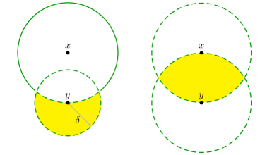
Figure 2. The regions ${\sf lune}(x,y,\delta)$ and ${\sf lens}(x,y)$

Let $P\subset\mathbb{R}^{2}$ be a finite set of points in the plane. Toussaint [35] defined the relative neighbourhood graph of $P$, denoted by ${\sf RNG}(P)$, to be the graph with vertex set $P$, where two vertices $v,w\in P$ are adjacent if and only if ${\sf lens}(x,y)\cap P=\emptyset$. That is $v$ and $w$ are adjacent whenever no vertex is simultaneously closer to $v$ than $w$ and closer to $w$ than $v$. Toussaint [35] proved that ${\sf MST}(P)\subseteq{\sf RNG}(P)$. Hence if ${\sf RNG}(P)$ is a tree, then ${\sf RNG}(P)={\sf MST}(P)$. The result of Monma and Suri [31] mentioned in Section 1 was strengthened by Bose et al. [4] as follows.

Lemma 2.1 (Bose et al. [4]).

Every degree-$5$ tree has a drawing that is the relative neighbourhood graph of its vertex set.

For all of the theorems introduced in Section 1, we in fact prove stronger results about relative neighbourhood graphs.

3. Drawings Based on a Partition

Theorem 1.1 is implied by the following result, since a relative neighbourhood graph that is a tree is a minimum spanning tree.

Theorem 3.1.

Let $\{T_{1},\dots,T_{k}\}$ be a partition of a tree $T$ into degree-$5$ subtrees. Then there is a drawing of $T$ in which each $T_{i}$ is drawn as the relative neighbourhood graph of its vertex set.

Proof.

Let $D$ be the maximum distance between any two vertices in $T$ (the diameter of $T$). Let $Q$ be the complete $5$-ary tree of height $D$. That is, every non-leaf vertex in $Q$ has degree $5$, and for some vertex $r$, the distance between $r$ and every leaf equals $D$.

By Lemma 2.1, there is a drawing of $Q$ that is the relative neighbourhood graph of its vertex set. Since the vertices of $Q$ are in general position, for some $\varepsilon>0$, for all distinct vertices $x,y\in V(Q)$, the discs ${\sf disc}(x,\varepsilon)$ and ${\sf disc}(y,\varepsilon)$ are disjoint, and if $P$ is a point set that contains exactly one point from each disc ${\sf disc}(x,\varepsilon)$ (where $x\in V(Q)$), then $Q\cong{\sf RNG}(P)$. (Here ${\sf disc}(x,\varepsilon)$ means the disc centred at the point where $x$ is drawn.)

Define a homomorphism $f$ from $T$ to $Q$ as follows. Choose an arbitrary starting vertex $v$ of $T$, let $f(v)=r$, and recursively construct a function $f$ such that $f(v)f(w)$ is an edge of $Q$ for every edge $vw$ of $T$, and if $f(v)f(w)=f(v^{\prime})f(w^{\prime})$ for distinct edges $vw\in E(T_{i})$ and $v^{\prime}w^{\prime}\in E(T_{j})$, then $i\neq j$. That is, edges in the same subtree are mapped to distinct edges of $Q$. Hence for each subtree $T_{i}$ of $T$, no two vertices in $T_{i}$ are mapped to the same vertex in $Q$ (otherwise the image of the path in $T_{i}$ between the two vertices would form a cycle in $Q$). Moreover, if $Q_{i}$ is the subgraph of $Q$ induced by $\{f(v):v\in V(T_{i})\}$ then $Q_{i}\cong T_{i}$. Draw each vertex $v\in V(T)$ at a distinct point $\phi(v)\in{\sf disc}(f(v),\varepsilon)$ so that $\{\phi(v):v\in V(T)\}$ is in general position. Thus $P_{i}:=\{\phi(v):v\in V(T_{i})\}$ contains exactly one point from each disc ${\sf disc}(x,\varepsilon)$ where $x\in V(Q_{i})$. Hence $T_{i}\cong Q_{i}\cong{\sf RNG}(P_{i})$ as desired. ∎

Theorem 1.2 is implied by the following stronger result.

Theorem 3.2.

Let $\{T_{1},\dots,T_{k}\}$ be a partition of a rooted tree $T$ into outdegree-$4$ subtrees. Then there is a non-crossing drawing of $T$ such that each $T_{i}$ is drawn as the relative neighbourhood graph of its vertex set.

Theorem 3.2 is proved by induction with the following hypothesis. This proof method generalises that of Bose et al. [4].

Lemma 3.3.

Let $\{T_{1},\dots,T_{k}\}$ be a partition of a rooted tree $T$ into outdegree-$4$ subtrees. Let $r$ be the root of $T$. Let $p$ and $q$ be distinct points in the plane. Let $\delta$ be a real number with $0<\delta<|pq|$. Then there is a non-crossing drawing of $T$ contained in ${\sf lune}(p,q,\delta)$ such that:

• $r$, which is drawn at $q$, is in ${\sf lens}(x,p)$ for every vertex $x$ of $T-r$, and

• for all $i\in\{1,\dots,k\}$, the subtree $T_{i}$ is drawn as the relative neighbourhood graph of its vertex set.

Proof.

We proceed by induction on $|V(T)|$. The result is trivial if $|V(T)|=1$. Now assume that $|V(T)|\geq 2$. Let $\delta^{\prime}$ be a real number with $0<\delta^{\prime}<\delta$. The circular arc $A:={\sf circle}(q,\delta^{\prime})-{\sf disc}(p,|pq|)$ has an angle (measured from $q$) greater than $\pi$. Thus, as illustrated in Figure 3, there are four points $s_{1},s_{2},s_{3},s_{4}$ in the interior of $A$, such that the angle (measured from $q$) between distinct points $s_{i}$ and $s_{j}$ is greater than $\frac{\pi}{3}$, implying $|s_{i}q|=|s_{j}q|<|s_{i}s_{j}|$ and $q\in{\sf lens}(s_{i},s_{j})$, and ${\sf lens}(q,s_{i})\cap\{s_{1},s_{2},s_{3},s_{4}\}=\emptyset$.

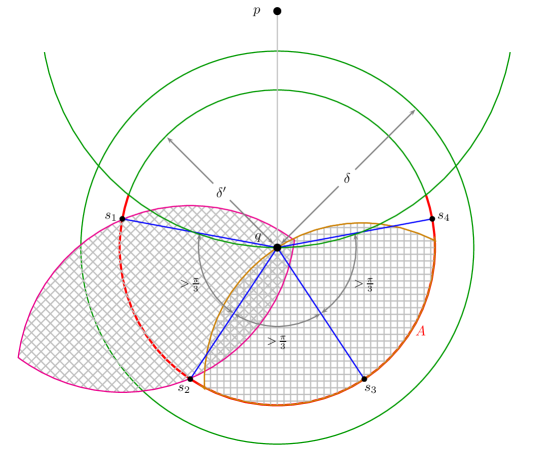
Figure 3. The points $s_{1},s_{2},s_{3},s_{4}$, showing that $q\in{\sf lens}(s_{1},s_{2})$ and ${\sf lens}(q,s_{3})\cap\{s_{1},s_{2},s_{3},s_{4}\}=\emptyset$.

For small enough discs around the $s_{i}$, these properties are extended to every point in the disc. More precisely, there is a real number $\varepsilon\in(0,\delta^{\prime})$ such that:

1. ${\sf disc}(s_{i},\varepsilon)\subset{\sf lune}(p,q,\delta)$ for all $i\in\{1,2,3,4\}$;

2. $q\in{\sf lens}(x,y)$ for all points $x\in{\sf disc}(s_{i},\varepsilon)$ and $y\in{\sf disc}(s_{j},\varepsilon)$ for all distinct $i,j\in\{1,2,3,4\}$;

3. $q\not\in{\sf lens}(x,y)$ for all points $x,y\in{\sf disc}(s_{i},\varepsilon)$ for all $i\in\{1,2,3,4\}$; and

4. ${\sf lens}(x,y)\cap{\sf disc}(s_{j},\varepsilon)=\emptyset$ for all points $x,y\in{\sf disc}(s_{i},\varepsilon)$ and for all distinct $i,j\in\{1,2,3,4\}$.

For $j\in\{1,2,3,4\}$, since ${\sf disc}(s_{j},\varepsilon)$ has diameter $2\varepsilon$, there are points $t_{j,1},\dots,t_{j,k}$ on the arc $A\cap{\sf disc}(s_{j},\varepsilon)$ such that discs of radius $\frac{\varepsilon}{k}$ centred at $t_{j,1},\dots,t_{j,k}$ are pairwise disjoint, as illustrated in Figure 4.

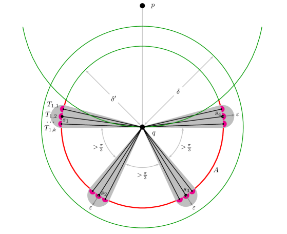
Figure 4. Construction in the proof of Lemma 3.3.

For $i\in\{1,\dots,k\}$, let $d_{i}$ be the outdegree of $r$ in $T_{i}$. So $d_{i}\in\{0,1,2,3,4\}$. Let $v_{i,1},\dots,v_{i,d_{i}}$ be the neighbours of $r$ in $T_{i}$. For $j\in\{1,\dots,d_{i}\}$, let $T_{i,j}$ be the component of $T-r$ that contains $v_{i,j}$. So $T_{i,j}$ is rooted at $v_{i,j}$, and $\{T_{1}\cap T_{i,j},\dots,T_{k}\cap T_{i,j}\}$ is a partition of $T_{i,j}$ into outdegree-$4$ subtreess. By induction, there is a non-crossing drawing of each $T_{i,j}$ contained in ${\sf lune}(q,t_{j,i},\frac{\varepsilon}{k})$ such that:

1. $v_{i,j}$, which is drawn at $t_{j,i}$, is in ${\sf lens}(x,q)$ for every vertex $x$ of $T_{i,j}-v_{i,j}$, and

2. for all $\ell\in\{1,\dots,k\}$, the subtree $T_{\ell}\cap T_{i,j}$ is drawn as the relative neighbourhood graph of its vertex set.

Draw $r$ at $q$, and draw a straight-line edge from $r$ to each neighbour $v_{i,j}$ of $r$. Each subtree $T_{i,j}$ is drawn outside of ${\sf disc}(q,\delta^{\prime})$, while the edges incident to $r$ are contained within ${\sf disc}(q,\delta^{\prime})$, and therefore do not cross any other edge. Hence the drawing of $T$ is non-crossing. By (a), $T_{i,j}$ is drawn within ${\sf lune}(q,t_{j,i},\frac{\varepsilon}{k})\subset{\sf disc}(t_{j},\varepsilon)\subset{\sf lune}(p,q,\delta)$. The edges incident to $r$ are drawn within ${\sf lune}(p,q,\delta)$. Hence all of $T$ is drawn within ${\sf lune}(p,q,\delta)$.

Now consider a vertex $x$ of $T-r$. Then $x$ is in $T_{i,j}$ for some $i\in\{1,2\dots,k\}$ and $j\in\{1,\dots,d_{i}\}$. Thus $x$ is drawn in ${\sf disc}(q,\delta)-{\sf disc}(p,|pq|)$, implying $|xq|<\delta<|xp|$ and $|pq|<|px|$. Hence $q\in{\sf lens}(x,p)$, implying $r\in{\sf lens}(x,p)$. This proves the first claim of the induction hypothesis.

It remains to prove that each subtree $T_{i}$ is drawn as the relative neighbourhood graph of its vertex set. Consider distinct vertices $v$ and $w$ in $T_{i}$. We must show that ${\sf lens}(v,w)\cap V(T_{i})=\emptyset$ if and only if $vw\in E(T_{i})$. Without loss of generality, $w\neq r$.

Case 1. $v=r$ and $vw\in E(T_{i})$: So $w=v_{i,j}$ for some $j\in\{1,2,3,4\}$. Then $v$ is drawn at $q$, and $w$ is drawn at $t_{j,i}$ . Now ${\sf lens}(q,t_{j,i})\subset{\sf disc}(q,\delta^{\prime})$, which contains no vertex except $r$ (at $q$). Thus ${\sf lens}(v,w)\cap V(T)=\emptyset$, as desired.

Case 2. $v=r$ and $vw\not\in E(T_{i})$: Then $w$ is in $T_{i,j}$ for some $j\in\{1,2,3,4\}$. Since $v$ is drawn at $q$, by induction, the vertex $t_{j,i}$, which is in $T_{i}$, is in ${\sf lens}(v,w)$, as desired.

Now assume that $v\neq r$ and $w\neq r$.

Case 3. $v$ and $w$ are in the same component $T_{\ell,j}$ of $T-r$: Then $v$ and $w$ are drawn within ${\sf disc}(t_{\ell},\varepsilon)$. Each vertex in $T_{i}$ is $r$, is in $T_{\ell,j}$, or is in $T_{i,j^{\prime}}$ for some $j^{\prime}\neq j$. Since $r$ is drawn at $q$, (c) implies that $r\not\in{\sf lens}(v,w)$. Since $T_{i,j^{\prime}}$ is drawn within ${\sf disc}(t_{j^{\prime},i},\varepsilon)$, by (d), ${\sf lens}(v,w)\cap V(T_{i,j^{\prime}})=\emptyset$. Hence ${\sf lens}(v,w)\cap V(T_{i})=\emptyset$ if and only if ${\sf lens}(v,w)\cap V(T_{\ell,j})\cap T_{i}=\emptyset$. By induction, ${\sf lens}(v,w)\cap V(T_{i})=\emptyset$ if and only if $v$ and $w$ are adjacent in $T_{i}$, as desired.

Case 4. $v$ and $w$ are in distinct components of $T-r$: Thus $r$ is in $T_{i}$, $v$ is in $T_{i,j}$ and $w\in T_{i,j^{\prime}}$ for some $j\neq j^{\prime}$, and $v$ and $w$ are not adjacent. By construction, $v$ is drawn in ${\sf disc}(s_{j},\varepsilon)$ and $w$ is drawn in ${\sf disc}(s_{j^{\prime}},\varepsilon)$. Thus (b) implies that $q\in{\sf lens}(v,w)$. Thus $r$, which is drawn at $q$, is in ${\sf lens}(v,w)$, as desired. ∎

4. Drawings with Large Angular Resolution

Theorem 1.3 is implied by the following stronger result:

Theorem 4.1.

Let $\{T_{1},\dots,T_{k}\}$ be a partition of a rooted tree $T$ into outdegree-$3$ subtrees. Then there is a non-crossing drawing of $T$ with angular resolution at least $\frac{\pi}{\max\{\Delta^{+}(T)-1,4\}}$ such that each subtree $T_{i}$ is drawn as the relative neighbourhood graph of its vertex set.

Theorem 4.1 is proved by induction with the following hypothesis.

Lemma 4.2.

Let $\{T_{1},\dots,T_{k}\}$ be a partition of a rooted tree $T$ into outdegree-$3$ subtrees. Let $r$ be the root of $T$. Let $p$ and $q$ be distinct points in the plane. Let $\delta$ be a real number with $0<\delta<|pq|$. Then there is a non-crossing drawing of $T$ contained in ${\sf lune}(p,q,\delta)$ such that:

• $r$, which is drawn at $q$, is in ${\sf lens}(x,p)$ for every vertex $x$ of $T-r$, and

• for all $i\in\{1,\dots,k\}$, the subtree $T_{i}$ is drawn as the relative neighbourhood graph of its vertex set, and

• the drawing of $T$ has angular resolution greater than $\frac{\pi}{\max\{4,\Delta^{+}(T)-1\}}$.

Proof.

We proceed by induction on $|V(T)|$. The result is trivial if $|V(T)|=1$. Now assume that $|V(T)|\geq 2$. Let $\delta^{\prime}$ be a real number with $0<\delta^{\prime}<\delta$.

Let $d:=\operatorname{outdeg}(r)$. For $i\in\{1,\dots,k\}$, let $d_{i}$ be the outdegree of $r$ in $T_{i}$. So $d_{i}\in\{0,1,2,3\}$ and $d=\sum_{i=1}^{k}d_{i}$. Let $v_{i,1},\dots,v_{i,d_{i}}$ be the neighbours of $r$ in $T_{i}$. Let

$$X:=\{i:d_{i}=3\},\;\;\;Y:=\{i:d_{i}=2\},\;\;\;Z:=\{i:d_{i}=1\}\enspace.$$

Thus $d=3|X|+2|Y|+|Z|$. Partition $Z=Z^{\prime}\cup Z^{\prime\prime}$ such that $|Z^{\prime\prime}|\leq|Z^{\prime}|\leq|Z^{\prime\prime}|+1$.

The circular arc $A:={\sf circle}(q,\delta^{\prime})-{\sf disc}(p,|pq|)$ has an angle (measured from $q$) greater than $\pi$. Thus there are points $s_{1},\dots,s_{d}$ in this order on $A$ such that the angle (measured from $q$) between distinct points $s_{a}$ and $s_{b}$ is greater than $\frac{\pi|b-a|}{d-1}$.

Let $\preceq$ be the total ordering of the neighbours of $r$ such that $\{v_{i,1}:i\in X\}\preceq\{v_{i,1}:i\in Y\}\preceq\{v_{i,1}:i\in Z^{\prime}\}\preceq\{v_{i,2}:i\in X\}\preceq\{v_{i,2}:i\in Y\}\preceq\{v_{i,1}:i\in Z^{\prime\prime}\}\preceq\{v_{i,3}:i\in X\}$, where within each set, the vertices are ordered by their $i$-value. Draw the neighbours of $r$ in the order of $\preceq$ at $s_{1},\dots,s_{d}$. That is, the first vertex in $\preceq$ is drawn at $s_{1}$, the second vertex in $\preceq$ is drawn at $s_{2}$, and so on. Let $t_{i,j}$ be the point where $v_{i,j}$ is drawn.

Consider distinct vertices $v_{i,j}$ and $v_{i,\ell}$ in some subtree $T_{i}$ such that $\ell>j$. Say $t_{i,j}=s_{a}$ and $t_{i,\ell}=s_{b}$. Observe that $b-a\geq|X|+|Y|+|Z^{\prime\prime}|\geq|X|+|Y|+\tfrac{1}{2}(|Z|-1)\geq\tfrac{1}{3}(3|X|+2|Y|+|Z|-1)=\frac{d-1}{3}$. Hence the angle (measured from $q$) between $v_{i,j}$ and $v_{i,\ell}$ is greater than $\frac{\pi(d-1)/3}{d-1}=\frac{\pi}{3}$. This implies that $|t_{i,j}q|=|t_{i,\ell}q|<|t_{i,j}t_{i,\ell}|$. Thus $q\in{\sf lens}(t_{i,j},t_{i,\ell})$ and $t_{i,\ell}\not\in{\sf lens}(q,t_{i,j})$ and $t_{i,j}\not\in{\sf lens}(q,t_{i,\ell})$.

For small enough discs around $s_{1},\dots,s_{d}$, these properties are extended to every point in the disc. More precisely, there is a real number $\varepsilon\in(0,\delta^{\prime})$ such that:

1. ${\sf disc}(s_{a},\varepsilon)\subset{\sf lune}(p,q,\delta)$ for all $a\in\{1,\dots,d\}$;

2. $q\in{\sf lens}(x,y)$ for all points $x\in{\sf disc}(t_{i,j},\varepsilon)$ and $y\in{\sf disc}(t_{i,\ell},\varepsilon)$ for all distinct vertices $v_{i,j}$ and $v_{i,\ell}$ in the same subtree $T_{i}$;

3. $q\not\in{\sf lens}(x,y)$ for all points $x,y\in{\sf disc}(s_{a},\varepsilon)$ for all $a\in\{1,\dots,d\}$; and

4. ${\sf lens}(x,y)\cap{\sf disc}(s_{b},\varepsilon)=\emptyset$ for all distinct $a,b\in\{1,\dots,d\}$ and for all points $x,y\in{\sf disc}(s_{a},\varepsilon)$.

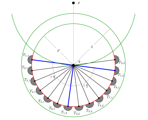
Figure 5. Construction in the proof of Lemma 4.2. Here $X=\{1,2\}$, $Y=\{3,4\}$, $Z^{\prime}=\{5,6\}$ and $Z^{\prime\prime}=\{7,8\}$. The tree $T_{1}$ is highlighted.

For $i\in\{1,\dots,k\}$ and $j\in\{1,\dots,d_{i}\}$, let $T_{i,j}$ be the component of $T-r$ that contains $v_{i,j}$. Each subtree $T_{i,j}$ is rooted at $v_{i,j}$, and $\{T_{1}\cap T_{i,j},\dots,T_{k}\cap T_{i,j}\}$ is a partition of $T_{i,j}$ into outdegree-$3$ subtreess. By induction, there is a non-crossing drawing of $T_{i,j}$ contained in ${\sf lune}(q,t_{i,j},\varepsilon)$ such that:

1. $v_{i,j}$, which is drawn at $t_{i,j}$, is in ${\sf lens}(x,q)$ for every vertex $x$ of $T_{i,j}-v_{i,j}$; and

2. for all $\ell\in\{1,\dots,k\}$, the subtree $T_{\ell}\cap T_{i,j}$ is drawn as the relative neighbourhood graph of its vertex set; and

3. the drawing of $T_{i,j}$ has angular resolution greater than $\frac{\pi}{\max\{\Delta^{+}(T_{i,j})-1,4\}}$, which is at least $\frac{\pi}{\max\{\Delta^{+}(T)-1,4\}}$.

Draw $r$ at $q$, and draw a straight-line edge from $r$ to each neighbour $v_{i,j}$ of $r$. The angle between two edges incident to $r$ is at least $\frac{\pi}{d-1}\geq\frac{\pi}{\Delta^{+}(T)-1}$. The angle between an edge $rv_{i,j}$ and each edge $v_{i,j}x$ in $T_{i,j}$ is at least $\frac{\pi}{4}$. With (g), this proves the third claim of the lemma.

Each subtree $T_{i,j}$ is drawn outside of ${\sf disc}(q,\delta^{\prime})$, while the edges incident to $r$ are contained within ${\sf disc}(q,\delta^{\prime})$, and therefore do not cross any other edge. Hence the drawing of $T$ is non-crossing. By (a), $T_{i,j}$ is drawn within ${\sf lune}(q,t_{i,j},\varepsilon)\subset{\sf disc}(t_{i,j},\varepsilon)\subset{\sf lune}(p,q,\delta)$. The edges incident to $r$ are drawn within ${\sf lune}(p,q,\delta)$. Hence all of $T$ is drawn within ${\sf lune}(p,q,\delta)$.

Now consider a vertex $x$ of $T-r$. Then $x$ is in $T_{i,j}$ for some $i\in\{1,\dots,k\}$ and $j\in\{1,\dots,d_{i}\}$. Thus $x$ is drawn in ${\sf disc}(q,\delta)-{\sf disc}(p,|pq|)$, implying $|xq|<\delta<|xp|$ and $|pq|<|px|$. Hence $q\in{\sf lens}(x,p)$, implying $r\in{\sf lens}(x,p)$. This proves the first claim of the lemma.

It remains to prove that each subtree $T_{i}$ is drawn as the relative neighbourhood graph of its vertex set. Consider distinct vertices $v$ and $w$ in $T_{i}$. We must show that ${\sf lens}(v,w)\cap V(T_{i})=\emptyset$ if and only if $vw\in E(T_{i})$. Without loss of generality, $w\neq r$.

Case 1. $v=r$ and $vw\in E(T_{i})$: So $w=v_{i,j}$ for some $j\in\{1,2,3\}$. Then $v$ is drawn at $q$, and $w$ is drawn at $t_{i,j}$ . Now ${\sf lens}(q,t_{i,j})\subset{\sf disc}(q,\delta^{\prime})$, which contains no vertex except $r$ (at $q$). Thus ${\sf lens}(v,w)\cap V(T)=\emptyset$, as desired.

Case 2. $v=r$ and $vw\not\in E(T_{i})$: Then $w$ is in $T_{i,j}$ for some $j\in\{1,2,3\}$, but $w\neq v_{i,j}$. Since $v$ is drawn at $q$, by (e), the vertex $v_{i,j}$, which is in $T_{i}$, is in ${\sf lens}(v,w)$, as desired.

Now assume that $v\neq r$ and $w\neq r$.

Case 3. $v$ and $w$ are in the same component $T_{\ell,j}$ of $T-r$, for some $\ell\in\{1,\dots,k\}$: Then $v$ and $w$ are drawn within ${\sf disc}(t_{\ell,j},\varepsilon)$. Each vertex in $T_{i}$ is $r$, is in $T_{\ell,j}$, or is in $T_{i,j^{\prime}}$ for some $(i,j^{\prime})\neq(\ell,j)$. Since $r$ is drawn at $q$, (c) implies that $r\not\in{\sf lens}(v,w)$. Since $T_{i,j^{\prime}}$ is drawn within ${\sf disc}(t_{i,j^{\prime}},\varepsilon)$, by (d), ${\sf lens}(v,w)\cap V(T_{i,j^{\prime}})=\emptyset$. Hence ${\sf lens}(v,w)\cap V(T_{i})=\emptyset$ if and only if ${\sf lens}(v,w)\cap V(T_{\ell,j})\cap T_{i}=\emptyset$. By (f), ${\sf lens}(v,w)\cap V(T_{i})=\emptyset$ if and only if $v$ and $w$ are adjacent in $T_{i}$, as desired.

Case 4. $v$ and $w$ are in distinct components of $T-r$: Thus $r$ is in $T_{i}$, $v$ is in $T_{i,j}$ and $w\in T_{i,j^{\prime}}$ for some $j\neq j^{\prime}$, and $v$ and $w$ are not adjacent. By construction, $v$ is drawn in ${\sf disc}(t_{i,j},\varepsilon)$ and $w$ is drawn in ${\sf disc}(t_{i,j^{\prime}},\varepsilon)$. Thus (b) implies that $q\in{\sf lens}(v,w)$. Thus $r$, which is drawn at $q$, is in ${\sf lens}(v,w)$, as desired.

Therefore the subtree $T_{i}$ is drawn as the relative neighbourhood graph of its vertex set. This completes the proof. ∎

5. Drawings Based on a Covering

Theorem 5.2 below establishes a result for relative neighbourhood graphs that implies Theorem 1.4 for minimum spanning trees. Before proving Theorem 5.2 we give a simpler proof of a weaker result, in which the obtained drawing might have crossings.

Proposition 5.1.

Let $\{T_{1},T_{2}\}$ be a covering of a tree $T$ by degree-$5$ subtrees. Then there is a drawing of $T$ in which each $T_{i}$ is drawn as the relative neighbourhood graph of its vertex set.

Proof.

We proceed by induction on $|V(T)|$. If $\Delta(T)\leq 5$ then $T\cong{\sf RNG}(P)$ for some point set $P$ by Lemma 2.1. This drawing is crossing-free since it also a minimum spanning tree. Furthermore, each $T_{i}$ is drawn as the relative neighbourhood graph of the subset of $P$ representing $T_{i}$. Now assume that $\Delta(T)\geq 6$. Thus $\deg_{T}(v)\geq 6$ for some vertex $v$. Hence there are edges $vx\in E(T_{1})-E(T_{2})$ and $vy\in E(T_{2})-E(T_{1})$. Let $T^{\prime}$ be the tree obtained from $T$ by identifying $x$ and $y$ into a new vertex $w$. (This operation is called an elementary homomorphism or folding; see [10, 21, 22, 5] and Figure 6.) Let $T^{\prime}_{i}$ be the subtrees of $T^{\prime}$ determined by $T_{i}$ for $i\in\{1,2\}$. Note that the edge $vw$ is in $T_{1}^{\prime}\cap T_{2}^{\prime}$. Observe that $\{T_{1}^{\prime},T_{2}^{\prime}\}$ is a covering of $T^{\prime}$ by degree-$5$ subtrees. By induction, there is a drawing of $T^{\prime}$ such that each $T_{i}^{\prime}$ is the relative neighbourhood graph of its vertex set. Moreover, for some $\varepsilon>0$, if $w$ is moved to any point in ${\sf disc}(w,\varepsilon)$ then in the resulting drawing of $T^{\prime}$, each $T_{i}^{\prime}$ is drawn as the relative neighbourhood graph of its vertex set. Consider a drawing of $T$ in which every vertex in $V(T)-\{x,y\}$ inherits is position in the drawing of $T^{\prime}$, and $x$ and $y$ are assigned distinct points in ${\sf disc}(w,\varepsilon)$. Since $x\in V(T_{1})-V(T_{2})$ and $y\in V(T_{2})-V(T_{1})$, each $T_{i}$ is drawn as the relative neighbourhood graph of its vertex set in the drawing of $T$. ∎

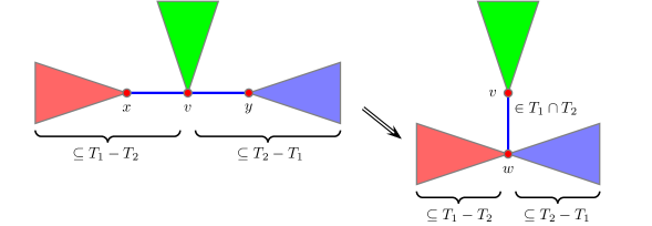
Figure 6. Folding the tree $T$ in the proof of Proposition 5.1.

We now strengthen Proposition 5.1 by showing that the drawing of $T$ can be made crossing-free. Theorem 1.4 is implied by the following stronger result:

Theorem 5.2.

Let $\{T_{1},T_{2}\}$ be a covering of a tree $T$ by degree-$5$ subtrees. Then there is a non-crossing drawing of $T$ such that each $T_{i}$ is drawn as the relative neighbourhood graph of its vertex set.

The proof of Theorem 5.2 depends on the following definition. A combinatorial embedding of a graph is a cyclic ordering of the edges incident to each vertex. We define a combinatorial embedding of a graph $G$, with respect to a covering $\{G_{1},G_{2}\}$ of $G$, to be good if for each vertex $v$ of $G$, in the clockwise ordering of the edges incident to $v$, the edges in $E(G_{1})-E(G_{2})$ are grouped together, followed by the edges in $E(G_{1})\cap E(G_{2})$, followed by the edges in $E(G_{2})-E(G_{1})$. Since every tree, covered by two subtrees, obviously has a good embedding, Theorem 5.2 now follows from the next lemma:

Lemma 5.3.

Let $\{T_{1},T_{2}\}$ be a covering of a tree $T$ by degree-$5$ subtrees. For every good combinatorial embeddding of $T$, with respect to $\{T_{1},T_{2}\}$, there is a non-crossing drawing of $T$ such that each $T_{i}$ is drawn as the relative neighbourhood graph of its vertex set, and the given combinatorial embedding of $T$ is preserved in the drawing.

Proof.

We proceed by induction on $|V(T)|$. If $\Delta(T)\leq 5$ then $T\cong{\sf RNG}(P)$ for some point set $P$ by Lemma 2.1. This drawing is crossing-free since it also a minimum spanning tree. Moreover, by examining the proof of Lemma 2.1, it is easily seen that any given combinatorial embedding of $T$ can be preserved in the drawing. Each $T_{i}$ is drawn as the relative neighbourhood graph of the subset of $P$ representing $T_{i}$. Now assume that $\deg_{T}(v)\geq 6$ for some vertex $v$. Hence there are edges $vx\in E(T_{1})-E(T_{2})$ and $vy\in E(T_{2})-E(T_{1})$ such that $vx$ and $vy$ are consecutive in the cyclic ordering of the edges incident to $v$.

Let $T^{\prime}$ be the tree obtained from $T$ by identifying $x$ and $y$ into a new vertex $w$. Let $T^{\prime}_{i}$ be the subtrees of $T^{\prime}$ determined by $T_{i}$ for $i\in\{1,2\}$. Note that the edge $vw$ is in $T_{1}^{\prime}\cap T_{2}^{\prime}$. The cyclic ordering of the edges in $T^{\prime}$ incident to $v$ is obtained from the cyclic ordering of the edges in $T$ incident to $v$ by replacing $vx$ and $vy$ (which are consecutive) by $vw$. And $N_{T^{\prime}}(w)$ is ordered $(N_{T_{1}-E(T_{2})}(x),wv,N_{T_{2}-E(T_{1})}(y))$. Other vertices keep their ordering in $T$.

Observe that $\{T_{1}^{\prime},T_{2}^{\prime}\}$ is a covering of $T^{\prime}$ by degree-$5$ subtrees. By induction, there is a non-crossing drawing of $T^{\prime}$ such that each $T_{i}^{\prime}$ is the relative neighbourhood graph of its vertex set, and the given combinatorial embedding of $T$ is preserved in the drawing. For some $\varepsilon>0$, if $w$ is moved to any point in ${\sf disc}(w,\varepsilon)$ then in the resulting drawing of $T^{\prime}$, each $T_{i}^{\prime}$ is drawn as the relative neighbourhood graph of its vertex set, and the given combinatorial embedding of $T$ is preserved. Consider a drawing of $T$ in which every vertex in $V(T)-\{x,y\}$ inherits is position in the drawing of $T^{\prime}$, and $x$ and $y$ are assigned distinct points in ${\sf disc}(w,\varepsilon)$. Since $x\in V(T_{1})-V(T_{2})$ and $y\in V(T_{2})-V(T_{1})$, each $T_{i}$ is drawn as the relative neighbourhood graph of its vertex set in the drawing of $T$. It remains to assign points for $x$ and $y$ in ${\sf disc}(w,\varepsilon)$ so that the drawing of $T$ is crossing-free. In the drawing of $T^{\prime}$, the edges incident to $w$ are ordered $(N_{T_{1}-E(T_{2})}(x),wv,N_{T_{2}-E(T_{1})}(y))$. Let $R$ be a ray centred at $w$ that separates the edges in $T_{1}-E(T_{2})$ incident to $w$ and those in $T_{2}-E(T_{1})$ incident to $w$, such that $v$ is not on the extension of $R$. At most one of $x$ and $y$, say $x$, has neighbours on both sides of the extension of $R$. As illustrated in Figure 7, position $x$ at $w$, and position $y$ on $R$ and inside ${\sf disc}(w,\varepsilon)$. It follows that there are no crossings and the correct ordering of edges is preserved at $v$, $x$ and $y$. ∎

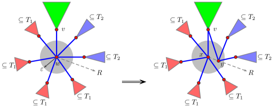
Figure 7. Producing a drawing of $T$ given a drawing of $T^{\prime}$ in the proof of Lemma 5.3.

We now show that Theorem 1.4 cannot be generalised for coverings by three or more subtrees. (Thus neither Proposition 5.1 nor Theorem 5.2 can be similarly generalised.) Let $T$ be the $6$-star with root $r$ and leaves $v_{1},\dots,v_{6}$. Let $\{T_{1},T_{2},T_{3}\}$ be the following covering of $T$. Let $T_{1}$ be the subtree of $T$ induced by $\{r,v_{1},v_{2},v_{3},v_{4}\}$. Let $T_{2}$ be the subtree of $T$ induced by $\{r,v_{1},v_{2},v_{5},v_{6}\}$. Let $T_{3}$ be the subtree of $T$ induced by $\{r,v_{3},v_{4},v_{5},v_{6}\}$. Thus each $T_{i}$ is a $4$-star. Suppose on the contrary that $T$ has a drawing such that each $T_{i}$ is drawn as a minimum spanning tree of its vertex set. The angle $\angle v_{i}rv_{j}$ between some pair of consecutive edges $rv_{i}$ and $rv_{j}$ (in the cyclic order around $r$) is less than $\frac{\pi}{3}$ since no three vertices are collinear. Since $v_{i}$ and $v_{j}$ are each in two subtrees, and $r$ is in every subtree, the vertices $r,v_{i},v_{j}$ are in a common subtree $T_{\ell}$. Every minimum spanning tree has angular resolution at least $\frac{\pi}{3}$. Thus $T_{\ell}$ is not drawn as a minimum spanning tree. This contradiction proves there is no drawing of $T$ such that each $T_{i}$ is drawn as a minimum spanning tree of its vertex set. Note that this argument generalises to show that if $P_{1},\dots,P_{15}$ are the $\binom{6}{2}$ paths through the root of the $6$-star $T$, then in every drawing of $T$, some $P_{i}$ is not a minimum spanning tree of its vertex set.

6. Further Research

This paper has not analysed the area of the drawings produced by our algorithms. It would be interesting to consider whether there are drawings whose area is polynomial in the number of vertices of the given tree, for example when the tree is partitioned into outdegree-3 subtrees. While the problem of drawing a tree as a minimum spanning tree in polynomial area is open in the general case [31], Kaufmann [26] proved that every degree-4 tree has a drawing as a minimum spanning tree in polynomial area; also see [32].

A second direction for further research is to extend the approach used in this paper to other types of proximity drawings of trees; see [30]. For example, every degree-4 tree admits a w-$\beta$-drawing for all values of $\beta$ in $(\cos(\frac{2\pi}{5})^{-1},\infty)$; see [12, Theorem 7]. Given a partition of a rooted tree $T$ into outdegree-3 subtrees and a value of $\beta$ in the above interval, is there a drawing of $T$ in which each subtree is drawn as a w-$\beta$-drawing?

The results of this paper motivate studying coverings and partitions of trees by subtrees of bounded degree. We consider these purely combinatorial problems in our companion paper [37]. For example, given a tree $T$ and integer $d$, we present there a formula for the minimum number of degree-$d$ subtrees that partition $T$, and describe a polynomial time algorithm that finds such a partition. Similarly, we present a polynomial time algorithm that finds a covering of $T$ by the minimum number of degree-$d$ subtrees.

References

- Aronov et al. [2009a] Boris Aronov, Muriel Dulieu, and Ferran Hurtado. Witness (Delaunay) graphs. In Proc. 7th Japan Conference on Computational Geometry and Graphs (JCCGG ’09). 2009a. http://arxiv.org/abs/1008.1053.
- Aronov et al. [2009b] Boris Aronov, Muriel Dulieu, and Ferran Hurtado. Witness (Gabriel) graphs. In Proc. 25th European Conference on Computational Geometry (EuroCG ’09), pp. 13–16. 2009b. http://arxiv.org/abs/1008.1051.
- Barát et al. [2006] János Barát, Jiří Matoušek, and David R. Wood. Bounded-degree graphs have arbitrarily large geometric thickness. Electron. J. Combin., 13(1):R3, 2006. http://www.combinatorics.org/Volume_13/Abstracts/v13i1r3.html%.
- Bose et al. [1996] Prosenjit Bose, William Lenhart, and Giuseppe Liotta. Characterizing proximity trees. Algorithmica, 16(1):83–110, 1996. http://dx.doi.org/10.1007/s004539900038.
- Buckley and Superville [1981] Fred Buckley and Lennox Superville. Extremal results for the ajointed number. In Proc. 12th Southeastern Conference on Combinatorics, Graph Theory and Computing, Vol. I, vol. 32 of Congr. Numer., pp. 163–171. 1981.
- Carmi et al. [2008] Paz Carmi, Vida Dujmović, Pat Morin, and David R. Wood. Distinct distances in graph drawings. Electron. J. Combin., 15:R107, 2008. http://www.combinatorics.org/Volume_15/Abstracts/v15i1r107.ht%ml.
- Chan [2002] Timothy M. Chan. A near-linear area bound for drawing binary trees. Algorithmica, 34(1):1–13, 2002. http://dx.doi.org/10.1007/s00453-002-0937-x.
- Chan et al. [2002] Timothy M. Chan, Michael T. Goodrich, S. Rao Kosaraju, and Roberto Tamassia. Optimizing area and aspect ratio in straight-line orthogonal tree drawings. Comput. Geom., 23(2):153–162, 2002. http://dx.doi.org/10.1016/S0925-7721(01)00066-9.
- Cohen et al. [1995] Robert F. Cohen, Giuseppe Di Battista, Roberto Tamassia, and Ioannis G. Tollis. Dynamic graph drawings: trees, series-parallel digraphs, and planar -digraphs. SIAM J. Comput., 24(5):970–1001, 1995. http://dx.doi.org/10.1137/S0097539792235724.
- Cook and Evans [1979] Curtis R. Cook and Anthony B. Evans. Graph folding. In Proc. 10th Southeastern Conference on Combinatorics, Graph Theory and Computing, vol. XXIII–XXIV of Congress. Numer., pp. 305–314. Utilitas Math., 1979.
- Crescenzi et al. [1992] Pilu Crescenzi, Giuseppe Di Battista, and Adolfo Piperno. A note on optimal area algorithms for upward drawings of binary trees. Comput. Geom., 2(4):187–200, 1992. http://dx.doi.org/10.1016/0925-7721(92)90021-J.
- Di Battista et al. [2006] Giuseppe Di Battista, Giuseppe Liotta, and Sue H. Whitesides. The strength of weak proximity. J. Discrete Algorithms, 4(3):384–400, 2006. http://dx.doi.org/10.1016/j.jda.2005.12.004.
- Dillencourt et al. [2000] Michael B. Dillencourt, David Eppstein, and Daniel S. Hirschberg. Geometric thickness of complete graphs. J. Graph Algorithms Appl., 4(3):5–17, 2000. http://www.cs.brown.edu/sites/jgaa/volume04.html.
- Dujmović et al. [2007] Vida Dujmović, David Eppstein, Matthew Suderman, and David R. Wood. Drawings of planar graphs with few slopes and segments. Comput. Geom. Theory Appl., 38:194–212, 2007. http://dx.doi.org/10.1016/j.comgeo.2006.09.002.
- Dujmović and Wood [2007] Vida Dujmović and David R. Wood. Graph treewidth and geometric thickness parameters. Discrete Comput. Geom., 37(4):641–670, 2007. http://dx.doi.org/10.1007/s00454-007-1318-7.
- Duncan [2009] Christian A. Duncan. On graph thickness, geometric thickness, and separator theorems. In Proc. 21st Canadian Conference on Computational Geometry (CCCG 2009), pp. 13–16. 2009. http://cccg.ca/proceedings/2009/cccg09_04.pdf.
- Duncan et al. [2004] Christian A. Duncan, David Eppstein, and Stephen G. Kobourov. The geometric thickness of low degree graphs. In Proc. 20th ACM Symp. on Computational Geometry (SoCG ’04), pp. 340–346. ACM Press, 2004. http://doi.acm.org/10.1145/997817.997868.
- Eades and Whitesides [1996] Peter Eades and Sue Whitesides. The realization problem for Euclidean minimum spanning trees is NP-hard. Algorithmica, 16(1):60–82, 1996. http://dx.doi.org/10.1007/s004539900037.
- Eppstein [2001] David Eppstein. Separating geometric thickness from book thickness, 2001. http://arxiv.org/abs/math/0109195.
- Eppstein [2004] David Eppstein. Separating thickness from geometric thickness. In János Pach, ed., Towards a Theory of Geometric Graphs, vol. 342 of Contemporary Mathematics, pp. 75–86. Amer. Math. Soc., 2004.
- Evans [1986] Anthony B. Evans. Absolutely -chromatic graphs. J. Graph Theory, 10(4):511–521, 1986. http://dx.doi.org/10.1002/jgt.3190100409.
- Gao and Hahn [1995] Guo-Gang Gao and Geňa Hahn. Minimal graphs that fold onto . Discrete Math., 142(1-3):277–280, 1995. http://dx.doi.org/10.1016/0012-365X(93)E0227-U.
- Garg and Rusu [2004] Ashim Garg and Adrian Rusu. Straight-line drawings of binary trees with linear area and arbitrary aspect ratio. J. Graph Algorithms Appl., 8(2):135–160, 2004. http://www.cs.brown.edu/sites/jgaa/volume08.html.
- Hong and Eades [2003] Seok-Hee Hong and Peter Eades. Drawing trees symmetrically in three dimensions. Algorithmica, 36(2):153–178, 2003. http://dx.doi.org/10.1007/s00453-002-1011-4.
- Hutchinson et al. [1999] Joan P. Hutchinson, Thomas C. Shermer, and Andrew Vince. On representations of some thickness-two graphs. Comput. Geom. Theory Appl., 13(3):161–171, 1999. http://dx.doi.org/10.1016/S0925-7721(99)00018-8.
- Kaufmann [2007] Michael Kaufmann. Polynomial area bounds for MST embeddings of trees. In Seok-Hee Hong, Takao Nishizeki, and Wu Quan, eds., Proc. 15th International Symposium on Graph Drawing (GD ’07), vol. 4875 of Lecture Notes in Computer Science, pp. 88–100. Springer, 2007. http://dx.doi.org/10.1007/978-3-540-77537-9_12.
- Kim [1997] Sung Kwon Kim. Logarithmic width, linear area upward drawing of AVL trees. Inform. Process. Lett., 63(6):303–307, 1997. http://dx.doi.org/10.1016/S0020-0190(97)00137-3.
- Kim [2004] Sung Kwon Kim. Order-preserving, upward drawing of binary trees using fewer bends. Discrete Appl. Math., 143(1–3):318–323, 2004. http://dx.doi.org/10.1016/j.dam.2004.02.011.
- Liotta and Meijer [2003] Giuseppe Liotta and Henk Meijer. Voronoi drawings of trees. Comput. Geom. Theory Appl., 24(3):147–178, 2003. http://dx.doi.org/10.1016/S0925-7721(02)00137-2.
- Liotta [pear] Guiseppe Liotta. Proximity drawings. In Roberto Tamassia, ed., Handbook of Graph Drawing and Visualization. CRC Press, to appear.
- Monma and Suri [1992] Clyde Monma and Subhash Suri. Transitions in geometric minimum spanning trees. Discrete Comput. Geom., 8(3):265–293, 1992. http://dx.doi.org/10.1007/BF02293049.
- Penna and Vocca [2004] Paolo Penna and Paola Vocca. Proximity drawings in polynomial area and volume. Comput. Geom. Theory Appl., 29(2):91–116, 2004. http://dx.doi.org/10.1016/j.comgeo.2004.03.015.
- Shin et al. [2000] Chan-Su Shin, Sung Kwon Kim, and Kyung-Yong Chwa. Area-efficient algorithms for straight-line tree drawings. Comput. Geom. Theory Appl., 15(4):175–202, 2000. http://dx.doi.org/10.1016/S0925-7721(99)00053-X.
- Suderman [2004] Matthew Suderman. Pathwidth and layered drawings of trees. Internat. J. Comput. Geom. Appl., 14(3):203–225, 2004. http://dx.doi.org/10.1142/S0218195904001433.
- Toussaint [1980] Godfried T. Toussaint. The relative neighbourhood graph of a finite planar set. Pattern Recognition, 12(4):261–268, 1980. http://dx.doi.org/10.1016/0031-3203(80)90066-7.
- Trevisan [1996] Luca Trevisan. A note on minimum-area upward drawing of complete and Fibonacci trees. Inform. Process. Lett., 57(5):231–236, 1996. http://dx.doi.org/10.1016/0020-0190(96)81422-0.
- Wood [2010] David R. Wood. Partitions and coverings of trees by bounded-degree subtrees. 2010.