Weak limits for exploratory plots in the analysis of extremes

Abstract

Exploratory data analysis is often used to test the goodness-of-fit of sample observations to specific target distributions. A few such graphical tools have been extensively used to detect subexponential or heavy-tailed behavior in observed data. In this paper we discuss asymptotic limit behavior of two such plotting tools: the quantile–quantile plot and the mean excess plot. The weak consistency of these plots to fixed limit sets in an appropriate topology of $\mathbb{R}^{2}$ has been shown in Das and Resnick (Stoch. Models 24 (2008) 103–132) and Ghosh and Resnick (Stochastic Process. Appl. 120 (2010) 1492–1517). In this paper we find asymptotic distributional limits for these plots when the underlying distributions have regularly varying right-tails. As an application we construct confidence bounds around the plots which enable us to statistically test whether the underlying distribution is heavy-tailed or not.

and

1 Introduction

Statistical analysis of extremes in available data has been very important in varied areas like finance (McNeil, Frey and Embrechts [28]), telecommunication (Maulik, Resnick and Rootzén [27], D’Auria and Resnick [10]), hydrology (Katz, Parlange and Naveau [24]), environmental statistics (Davison and Smith [11], Smith [39]) and many more. Before analyzing features of the data using extreme value analysis, it is imperative that we check whether extreme-value modeling is well suited in the given context; see Drees [17] for a recent survey of exploratory techniques for extremes in an actuarial context. Popular exploratory techniques in this direction have been the mean excess (ME) plots (Davison and Smith [11]) and the quantile–quantile (QQ) plots which are specifically tuned for heavy-tailed data (Kratz and Resnick [25]). A distribution $F$ is heavy-tailed if the tail probability $(1-F)$ is regularly varying (Resnick [34], Chapter 1). It has been shown earlier that under an assumption of heavy tails and with proper normalizations, both plots converge in probability to fixed closed sets (for ME plots, an additonal assumption of finiteness of the mean of $F$ is required); see Das and Resnick [9] and Ghosh and Resnick [22]. These results corroborate the use of the QQ plot and the ME plot to test the null hypothesis that the underlying distribution is heavy-tailed. The proximity of the observed plot to the fixed limit set would support the null hypothesis.

Incidentally, one data set leads to just one single plot of each kind. A single plot is often not enough to statistically detect proximity between the plot and the intended fixed limit set; see the examples in Section 6. Creating appropriate confidence bounds around these plots, though, can help us to test the null hypothesis with some degree of confidence. In this paper we study weak limits of both kinds of plots for heavy-tailed data and use these limits to obtain confidence bounds around them with asymptotic coverage probabilities. The methods used here are general and can be used to find weak limits and confidence bounds for other plots used in the analysis of extremes.

1.1 Plan for this paper

We introduce the two plotting methodologies in Section 1. In Section 2 we set up necessary tools to talk about convergence of random closed sets in $\mathbb{R}^{2}$, since the QQ and ME plots are random closed sets in $\mathbb{R}^{2}$. In Sections 3 and 4, we prove weak convergence of the QQ and the ME plot under the null hypothesis that the underlying distribution $F$ is heavy-tailed. We proceed by expressing both plots as appropriate functionals of the tail empirical measure and then use convergence properties of the tail empirical measure to prove weak convergence of both plots. As an application to obtaining these weak limits, we construct confidence bounds with asymptotic coverage probability for both kinds of plots in Section 5. Finally, in Section 6 we apply the results obtained in the previous sections to simulated and real data sets to exemplify how they perform in practice. We conclude in Section 7 along with a discussion on future directions.

1.2 QQ plots for heavy tails

Suppose we want to test the null hypothesis that observations from a sample are independent and identically distributed (i.i.d.) with some known distribution $F$. The QQ plot, which is a plot of the empirical quantiles from the data against the distributional quantiles of $F$, is an intuitive and popular graphical tool for detecting the goodness-of-fit for a sample to the distribution $F$. If the true distribution of the sample is $F$, then the QQ plot should converge, in an appropriate sense, to a straight line. Results involving empirical process and quantile process convergences are available in Shorack and Wellner [38], which can be appropriately used to create confidence intervals for QQ plots. The QQ plot we consider is a little different and is specifically designed to check for distributions $F$ where $\bar{F}:=1-F$ is regularly varying with some index $-1/\xi$, $\xi>0$, also denoted $\bar{F}\in RV_{-1/\xi}$ (Resnick [34], Chapter 1). For a sample $X_{1},X_{2},\ldots,X_{n}$, its decreasing order statistics are denoted by $X_{(1)}\geq X_{(2)}\geq\cdots\geq X_{(n)}$ and the QQ plot in this context is defined by

$$\mathcal{Q}_{n}=\biggl{\{}\biggl{(}-\log\frac{j}{k},\log\frac{X_{(j)}}{X_{(k)}}\biggr{)}\colon\ 1\leq j\leq k\biggr{\}},\qquad k<n.$$

Clearly we concentrate on the top $k$ quantiles of the data justified by the fact that $\bar{F}\in RV_{-1/\xi}$ only provides us with information about the right tail of the data. Under the null hypothesis of $\bar{F}\in RV_{-1/\xi}$ for some $\xi>0$, Das and Resnick [9] have shown convergence in probability for QQ plots in an appropriate topology of random closed sets when the data is assumed to be an i.i.d. sample.

1.3 ME plots

The ME function of a random variable $X$ is defined as

$$M(u):=E[X-u|X>u],$$ (1)

provided $EX_{+}<\infty,$ and is also known as the mean residual life function. A natural estimate of $M(u)$ is the empirical ME function $\hat{M}(u)$ defined as

$$\hat{M}(u)=\frac{\sum_{i=1}^{n}(X_{i}-u)I_{[X_{i}>u]}}{\sum_{i=1}^{n}I_{[X_{i}>u]}},\qquad u\geq 0.$$ (2)

The ME plot is the plot of the points $\{(X_{(k)},\hat{M}(X_{(k)}))\colon\ 1<k\leq n\}$.

The ME plot is often used as a simple graphical test to check if data conform to a generalized Pareto distribution (GPD). The GPD is an important class of distributions and is fundamental for the peaks-over-threshold method used in extreme value analysis (Davison and Smith [11]). The GPD is characterized by its cumulative distribution function $G_{\xi,\beta}$

$$G_{\xi,\beta}(x)=\cases{1-(1+\xi x/\beta)^{-1/\xi}&\quad$\mbox{if }\xi\neq 0,$\vspace*{2pt}\cr 1-\exp(-x/\beta)&\quad$\mbox{if }\xi=0,$}$$ (3)

where $\beta>0$, and $x\geq 0$, when $\xi\geq 0$ and $0\leq x\leq-\beta/\xi$, if $\xi<0$. The parameters $\xi$ and $\beta$ are referred to as the shape and the scale parameter, respectively. The GPD in the case $\xi>0$ corresponds to the classical Pareto law with tail exponent $1/\xi$. For a random variable $X\sim G_{\xi,\beta}$, we have $E(X)<\infty$, if and only if $\xi<1$, and in this case, the ME function of $X$ is linear in $u$.

$$M(u)=\frac{\beta}{1-\xi}+\frac{\xi}{1-\xi}u,$$ (4)

where $0\leq u<\infty$ if $0\leq\xi<1$ and $0\leq u\leq-\beta/\xi$ if $\xi<0$. In fact, the linearity of the ME function characterizes the GPD class; cf. McNeil, Frey and Embrechts [28] and Embrechts, Klüppelberg and Mikosch [18]. Davison and Smith [11] used this property and suggested that if the ME plot is close to a straight line for high values of the threshold, then there is no evidence against the use of a GPD model. See also Embrechts, Klüppelberg and Mikosch [18] and Hogg and Klugman [23] for the implementation of this plot in practice. Ghosh and Resnick [22] discuss convergence in probability for the high thresholds of suitably normalized ME plots in an appropriate topology of random closed sets when the data is an i.i.d. sample.

The advantage of the ME plot over the QQ plot is that it works when $-\infty<\xi<1$, whereas the QQ plot works for $\xi>0$ only. Hence the ME plot can be used whenever the sample is in the maximal domain of attraction of any generalized extreme value distribution with finite mean (Gumbel, Weibull or Fréchet distribution). The QQ plot is restricted to the domain of attraction of Fréchet distribution only. In this paper, though, we restrict to the case when $\xi>0$, which is the case of maximal domain of attraction of the Fréchet distribution. The disadvantage of the ME plot is that it requires $\xi<1$ to make proper sense of the result, that is, the underlying distribution should have a finite mean. Still, limits can and have been obtained for the ME plots, even when the distributional mean is not finite; see Ghosh and Resnick [22].

2 Preliminaries

2.1 Topology on closed sets of $\mathbb{R}^{2}$

Since we are dealing with plots which are closed sets in $\mathbb{R}^{2}$, it is imperative to understand the topology on closed sets. We denote the collection of all closed (compact) sets in $\mathbb{R}^{2}$ by $\mathcal{F}$ ($\mathcal{K}$, resp.). We consider a hit and miss topology on $\mathcal{F}$ called the Fell topology. The Fell topology is the smallest topology containing the families $\{\mathcal{F}^{K},K\mbox{ compact}\}$ and $\{\mathcal{F}_{G},G\mbox{ open}\}$ where, for any set $B$,

$$\mathcal{F}^{B}=\{F\in\mathcal{F}\colon\ F\cap B=\varnothing\}\quad\mbox{and}\quad\mathcal{F}_{B}=\{F\in\mathcal{F}\colon\ F\cap B\neq\varnothing\}.$$

Hence $\mathcal{F}^{B}$ and $\mathcal{F}_{B}$ are collections of closed sets which miss and hit the set $B$, respectively. This is the reason for which such topologies are called hit and miss topologies. In the Fell topology, a sequence of closed sets $\{F_{n}\}$ converges to $F\in\mathcal{F}$ if and only if the following two conditions hold:

• $F\in\mathcal{F}_{G}$ implies there exists $N\geq 1$ such that for all $n\geq N$, $F_{n}\in\mathcal{F}_{G}$, for any open set $G$.

• $F\in\mathcal{F}^{K}$ implies there exists $N\geq 1$ such that for all $n\geq N$, $F_{n}\in\mathcal{F}^{K}$, for any compact set $K$.

The Fell topology on the closed sets of $\mathbb{R}^{2}$ is metrizable (Flachsmeyer [19], Beer [1]) and we indicate convergence in this topology of a sequence $(F_{n})$ of closed sets to a limit closed set $F$ by $F_{n}\to F$. Often though, it is easier to deal with the following characterization of convergence.

Lemma 2.1

A sequence $F_{n}\in\mathcal{F}$ converges to $F\in\mathcal{F}$ in the Fell topology if and only if the following two conditions hold:

1. For any $t\in F$ there exists $t_{n}\in F_{n}$ such that $t_{n}\to t.$

2. If, for some subsequence $(m_{n})$, $t_{m_{n}}\in F_{m_{n}}$ converges, then $\lim_{n\to\infty}t_{m_{n}}\in F$.

See Theorem 1-2-2 in Matheron [26], page 6, for a proof of this lemma.

Let $\sigma_{\mathcal{F}}$ denote the Borel $\sigma$-algebra generated by the Fell topology of open sets (not to be confused with open sets in $\mathbb{R}^{d}$). A random closed set $X\mathchoice{\nobreak\,\colon}{\nobreak\,\colon}{\nobreak\,\colon\;}{\nobreak\,\colon\;}\Omega\mapsto\mathcal{F}$ is a measurable mapping from $(\Omega,\mathcal{A},P^{\prime})$ to $(\mathcal{F},\sigma_{\mathcal{F}})$. Denote by $P$ the induced probability on $\sigma_{\mathcal{F}}$, that is, $P=P^{\prime}\circ X^{-1}.$

Since the Fell topology is metrizable, the definition of convergence in probability is obvious. The following result is a well-known and helpful characterization for convergence in probability of random variables, and it holds for random sets as well; see Theorem 6.21 in Molchanov [29], page 92.

Lemma 2.2

A sequence of random sets $(F_{n})$ in $\mathcal{F}$ converges in probability to a random set $F$ if and only if for every subsequence $(n^{\prime})$ of $\mathbb{Z}_{+}$ there exists a further subsequence $(n^{\prime\prime})$ of $(n^{\prime})$ such that $F_{n^{\prime\prime}}\to F$-a.s.

A sequence of random closed sets $(X_{n})_{n\geq 1}$ weakly converges to a random closed set $X$ with distribution $P$ if the corresponding induced probability measures $(P_{n})_{n\geq 1}$ converge weakly to $P$, that is,

$$P_{n}(\mathcal{B})=P_{n}^{\prime}\circ X_{n}^{-1}(\mathcal{B})\quad\to\quad P(\mathcal{B})=P^{\prime}\circ X^{-1}(\mathcal{B}),\qquad\mbox{as }n\to\infty$$

for each $\mathcal{B}\in\sigma_{\mathcal{F}}$ such that $P(\partial\mathcal{B})=0$. This is not always straightforward to verify from the definition. The following characterization of weak convergence in terms of sup-measures is very useful; cf. Vervaat [42]. Suppose $h\mathchoice{\nobreak\,\colon}{\nobreak\,\colon}{\nobreak\,\colon\;}{\nobreak\,\colon\;}\mathbb{R}^{d}\to\mathbb{R}_{+}=[0,\infty)$. For $X\subset\mathbb{R}^{d}$, define $h(X)=\{h(x)\mathchoice{\nobreak\,\colon}{\nobreak\,\colon}{\nobreak\,\colon\;}{\nobreak\,\colon\;}x\in X\}$, and $h^{\vee}$ is the sup-measure generated by $h$ defined by

$$h^{\vee}(X)=\sup\{h(x)\mathchoice{\nobreak\,\colon}{\nobreak\,\colon}{\nobreak\,\colon\;}{\nobreak\,\colon\;}x\in X\}$$

(Molchanov [29], Vervaat [42]). These definitions permit the following characterization (Molchanov [29], page 87).

Lemma 2.3

A sequence $(X_{n})_{n\geq 1}$ of random closed sets converges weakly to a random closed set $X$ if and only if $\mathbb{E}h^{\vee}(X_{n})$ converges to $\mathbb{E}h^{\vee}(X)$ for every non-negative continuous function $h\mathchoice{\nobreak\,\colon}{\nobreak\,\colon}{\nobreak\,\colon\;}{\nobreak\,\colon\;}\mathbb{R}^{d}\to\mathbb{R}$ with a bounded support.

We often use the following notation: for a $x\in\mathbb{R}$ and a set $A\subset\mathbb{R}^{n}$, $xA=\{xy\colon\ y\in A\}$ and $x+A=\{x+y\colon\ y\in A\}$. See Matheron [26] and Molchanov [29] for further details on the theory of random sets.

2.2 Miscellany

Throughout this paper we will take $k:=k_{n}$ to be a sequence increasing to infinity such that $k_{n}/n\to 0$. For a distribution function $F(x)$ we write $\bar{F}(x):=1-F(x)$ for the tail, and the quantile function is

$$b(u):=F^{\leftarrow}\biggl{(}1-\frac{1}{u}\biggr{)}=\inf\biggl{\{}s\colon\ F(s)\geq 1-\frac{1}{u}\biggr{\}}=\biggl{(}\frac{1}{1-F}\biggr{)}^{\leftarrow}(u).$$

A function $U\mathchoice{\nobreak\,\colon}{\nobreak\,\colon}{\nobreak\,\colon\;}{\nobreak\,\colon\;}(0,\infty)\to\mathbb{R}_{+}$ is regularly varying with index $\rho\in\mathbb{R}$, written $U\in RV_{\rho}$, if

$$\lim_{t\to\infty}\frac{U(tx)}{U(t)}=x^{\rho},\qquad x>0.$$

Regular variation is discussed in several books such as Resnick [33, 34], Seneta [37], Geluk and de Haan [20], de Haan [12], de Haan and Ferreira [13], Bingham, Goldie and Teugels [3].

We use $M_{+}(0,\infty]$ to denote the space of non-negative Radon measures $\mu$ on $(0,\infty]$ metrized by the vague metric. Point measures are written as a function of their points $\{x_{i},i=1,\dots,n\}$ by $\sum_{i=1}^{n}\delta_{x_{i}};$ see, for example, Resnick [34], Chapter 3.

We will use the following notations to denote different classes of functions: For $0\leq a<b\leq\infty$,

1. $\mathbb{C}[a,b)$: Continuous functions on $[a,b)$.

2. $\mathbb{D}[a,b)$: Right-continuous functions with finite left limits defined on $[a,b)$.

3. $\mathbb{D}_{l}[a,b)$: Left-continuous functions with finite right limits defined on $[a,b)$.

$\mathbb{D}[0,1]$ is complete and separable under a metric $d_{0}(\cdot)$, which is equivalent to the Skorohod metric $d_{S}(\cdot)$ (Billingsley [2], page 128), but not under the uniform metric $\|\cdot\|$. As we will see, the limit processes that appear in our analysis below are always continuous. We can check that if $x$ is continuous (in fact, uniformly continuous) in $[0,1]$, for $x_{n}\in\mathbb{D}[0,1]$, $\|x_{n}-x\|\to 0$ is equivalent to $d_{S}(x_{n},x)\to 0$ and hence equivalent to $d_{0}(x_{n},x)\to 0$ as $n\to\infty$ (Billingsley [2], page 124). So we use convergence in uniform metric, for our convenience henceforth. For spaces of the form $\mathbb{D}[a,b)$ or $\mathbb{D}_{l}[a,b)$, we will consider the topology of locally uniform convergence. In some cases we will also consider product spaces of functions, and then the topology will be the product topology. For example, $\mathbb{D}^{2}_{l}[1,\infty)$ will denote the class of 2-dimensional functions on $[1,\infty)$ which are left-continuous with right limit. The classes of functions defined on the sets $[a,b]$ or $(a,b]$ will have the obvious notation.

2.3 A useful lemma

The following lemma will be used often in the proofs below. We use “$\Rightarrow$” to denote weak convergence.

Lemma 2.4

Let $Y_{n}\in\mathbb{D}^{2}_{l}(0,1]$ be a sequence of random functions and assume the following hold:

1. [(ii)]

2. $Y_{n}\Rightarrow Y$, where $Y(t)$ has continuous paths with probability 1.

3. There exists a partition $0=t^{(0)}_{n}<t_{n}^{(1)}<\cdots<t_{n}^{(m_{n})}=1$ such that $Y_{n}(t)$ is constant on the interval $(t_{n}^{(i)},t_{n}^{(i+1)}]$ for all $0\leq i<m_{n}$ with probability 1.

Then for any $0<\varepsilon<1$,

$$\mathcal{Y}^{\varepsilon}_{n}:=\bigl{\{}Y_{n}\bigl{(}t_{n}^{(i)}\bigr{)}\colon\ 0<i\leq m_{n},t_{n}^{(i)}\geq\varepsilon\bigr{\}}\quad\Rightarrow\quad\mathcal{Y}^{\varepsilon}:=\{Y(t)\colon\ \varepsilon\leq t\leq 1\}\qquad\mbox{in }\mathcal{F}.$$ (5)

Furthermore, if $\lim_{t\downarrow 0,n\to\infty}|Y_{n}(t)|=\infty$ with probability 1, then

$$\mathcal{Y}_{n}:=\bigl{\{}Y_{n}\bigl{(}t_{n}^{(i)}\bigr{)}\colon\ 0<i\leq m_{n}\bigr{\}}\quad\Rightarrow\quad\mathcal{Y}:=\{Y(t)\colon\ 0<t\leq 1\}\qquad\mbox{in }\mathcal{F}.$$ (6)

Proof.

Using Lemma 2.3 it suffices to show that

$$\lim_{n\rightarrow\infty}E[h^{\vee}(\mathcal{Y}_{n})]=E[h^{\vee}(\mathcal{Y})]$$

for any continuous function $h\mathchoice{\nobreak\,\colon}{\nobreak\,\colon}{\nobreak\,\colon\;}{\nobreak\,\colon\;}\mathbb{R}^{2}\mapsto\mathbb{R}_{+}$ with a compact support. So take any such function $h$. By the Skorohod representation theorem (Billingsley [2], Theorem 6.7, page 70), there exists a probability space $(\Omega,\mathcal{G},P)$ and random elements $Y_{n}^{*}$ and $Y^{*}$ in $\mathbb{D}^{2}_{l}(0,1]$ such that

$$Y_{n}^{*}\stackrel{{\scriptstyle d}}{{=}}Y_{n}\quad\mbox{and}\quad Y^{*}\stackrel{{\scriptstyle d}}{{=}}Y$$

in the sense of finite dimensional distributions (f.d.d.) and

$$Y_{n}^{*}\to Y^{*},\qquad P\mbox{-a.s. in }\mathbb{D}^{2}_{l}(0,1].$$

Now observe that

$$h^{\vee}(\mathcal{Y}^{\varepsilon})=\sup_{x\in\mathcal{Y}^{\varepsilon}}h(x)\stackrel{{\scriptstyle d}}{{=}}\sup_{\varepsilon\leq t\leq 1}h(Y^{*}(t))\quad\mbox{and}\quad h^{\vee}(\mathcal{Y}^{\varepsilon}_{n})=\sup_{x\in\mathcal{Y}^{\varepsilon}_{n}}h(x)\stackrel{{\scriptstyle d}}{{=}}\sup_{\varepsilon\leq t\leq 1}h(Y_{n}^{*}(t)).$$

Since $Y^{*}(t)$ is continuous, we know that $\sup_{\varepsilon\leq t\leq 1}|Y^{*}_{n}(t)-Y^{*}(t)|\to 0$. Moreover, since $h$ is continuous with a compact support, we get $h$ is uniformly continuous, and hence

$$\sup_{\varepsilon\leq t\leq 1}h(Y_{n}^{*}(t))\to\sup_{\varepsilon\leq t\leq 1}h(Y^{*}(t)),\qquad P\mbox{-a.s.}$$ (7)

As $h$ is bounded, applying the dominated convergence theorem, we get

$$E[h^{\vee}(\mathcal{Y}^{\varepsilon}_{n})]=E\Bigl{[}\sup_{\varepsilon\leq t\leq 1}h(Y_{n}^{*}(t))\Bigr{]}\rightarrow E\Bigl{[}\sup_{\varepsilon\leq t\leq 1}h(Y^{*}(t))\Bigr{]}=E[h^{\vee}(\mathcal{Y}^{\varepsilon})],$$

and this proves (5).

Since $h\mathchoice{\nobreak\,\colon}{\nobreak\,\colon}{\nobreak\,\colon\;}{\nobreak\,\colon\;}\mathbb{R}^{2}\mapsto\mathbb{R}_{+}$ has a bounded support, we can find $M>0$ such that $h(x)=0$ whenever $|x|>M$. If $\lim_{t\downarrow 0,n\to\infty}|Y^{*}_{n}(t)|=\infty$ with probability 1, then almost surely for any $\omega\in\Omega$ we can find $\delta>0$ and $N\geq 1$ such that $|Y^{*}_{n}(t)(\omega)|>M$ for all $\delta\leq t\leq 1$ and $n\geq N$. This implies (using (7))

$$\sup_{0<t\leq 1}h(Y_{n}^{*}(t)(\omega))=\sup_{\varepsilon\leq t\leq 1}h(Y_{n}^{*}(t)(\omega))\to\sup_{\varepsilon\leq t\leq 1}h(Y^{*}(t)(\omega))=\sup_{0<t\leq 1}h(Y^{*}(t)(\omega)).$$

The remaining part of the proof of (6) can be completed using the same argument used to prove (5). ∎

3 Limit results for the QQ plots

Convergence of empirical processes and quantile processes to functionals of Gaussian processes, usually Brownian motion and Brownian bridges, are quite well known; cf. Shorack and Wellner [38]. We prove similar results for extreme order statistics. We use the weak limit of tail empirical measure and deduce weak convergence of the logarithmic version of the QQ plot of the extreme order statistics as a random set.

The following was proved in Das and Resnick [9]:

Proposition 3.1

Suppose $X_{1},\ldots,X_{n}$ are i.i.d. with common distribution $F$, and $X_{(1)}\geq X_{(2)}\geq\cdots\geq X_{(n)}$ are the order statistics from this sample. If $F$ is strictly increasing and continuous on its support, then

$$\mathcal{T}_{n}:=\biggl{\{}\biggl{(}F^{\leftarrow}\biggl{(}\frac{i}{n+1}\biggr{)},X_{(n-i+1)}\biggr{)}\colon\ 1\leq i\leq n\biggr{\}}\quad\stackrel{{\scriptstyle P}}{{\to}}\quad\mathcal{T}:=\{(x,x)\colon\ x\in\operatorname{support}(F)\}$$

in $\mathcal{F}$.

This proposition though is not enough if one is interested in creating confidence bounds from the data. For that purpose one would need weak convergence results which are widely known in terms of convergence of affine transformations of quantile processes to appropriate Brownian Bridges for a known distribution $F$; see Shorack and Wellner [38], Chapter 3, for further details. In the following section, we concentrate on the case where $\bar{F}$ is regularly varying with tail index $-1/\xi$ with $\xi>0$. The specific form of $F$ is otherwise unknown.

3.1 QQ plots for distributions with regularly varying tails

Now assume that $X_{1},X_{2},\ldots,X_{n}$ are i.i.d. from a distribution $F$. Suppose we want to check whether $F$ is heavy-tailed or not. In the sense of testing a hypothesis, our null hypothesis is that $\bar{F}\in RV_{-1/\xi}$ for some $\xi>0$. Note that we really do not have any specific form for $F$. We define the following sets:

$$\mathcal{Q}_{n} = \biggl{\{}\biggl{(}-\log\frac{j}{k},\log\frac{X_{(j)}}{X_{(k)}}\biggr{)}\colon\ 1\leq j\leq k\biggr{\}},\qquad k<n,$$ (8)

$$\mathcal{Q} = \{(x,\xi x)\colon\ x\geq 0\}.$$ (9)

The set $\mathcal{Q}_{n}$ is the logarithmic version of the QQ plot for the first $k$ order statistics from the sample $X_{1},\ldots,X_{n}$.

Das and Resnick [9] proved that under the null hypothesis, $\mathcal{Q}_{n}\stackrel{{\scriptstyle P}}{{\to}}\mathcal{Q}$ in $\mathcal{F}$ as $k,n\to\infty$ with $k/n\to 0$. We show below that a distributional convergence can also be obtained in this case.

Assumption 3.2.

$F$ satisfies

$$\lim_{n\to\infty}\sqrt{k}\biggl{(}\frac{n}{k}\bar{F}\bigl{(}b(n/k)y^{-\xi}\bigr{)}-y\biggr{)}=0$$ (10)

locally uniformly on $(0,\infty]$ as $k,n,n/k\to\infty$.

Theorem 3.3

Suppose $X_{1},\ldots,X_{n}$ are i.i.d. observations from a distribution $F$ satisfying $\bar{F}\in RV_{-1/\xi}$ with $\xi>0$ and Assumption 3.2. Then as $n,k,n/k\to\infty$

$$\mathcal{QN}_{n}:=\biggl{\{}\biggl{(}-\log\frac{j}{k},-\xi\log\frac{j}{k}+\sqrt{k}\biggl{(}\log\frac{X_{(j)}}{X_{(k)}}+\xi\log\frac{j}{k}\biggr{)}\biggr{)}\colon\ 1\leq j\leq k\biggr{\}}$$

(11)

$$\quad\Rightarrow\quad\mathcal{QN}:=\bigl{\{}\bigl{(}-\log t,-\xi\log t+\xi t^{-1}B(t)\bigr{)}\colon\ 0<t\leq 1\bigr{\}}\qquad\mbox{in }\mathcal{F},$$

where $B(t)$ is a Brownian Bridge on $[0,1]$ restricted to $(0,1]$.

Remark 3.4.

The set $\mathcal{QN}_{n}$ is a suitably normalized version of the QQ plot which allows us to obtain a weak limit. It is important to observe that the format in which we have expressed the result is not standard in the literature as far as weak limits of random variables or functions are concerned. Usual weak limit results will only consider the normalized difference of the random variable from its mean or its limit in probability. In our setting it is imperative to state the result in the form which we have used. We look at the plot as the probability limit perturbed by the normalized deviation around it; that is, we shift the normalized differences so that we can obtain the distribution of the deviation of the observed points of the QQ plot from its mean position. If we do not make this shift, the weak limit will always hover around the $y$-axis and will not give the deviation from the actual point in the plot.

Remark 3.5.

We have used Assumption 3.2 in order to prove a weak limit for the QQ plots. Without this assumption we can show the convergence of tail empirical measure with unknown centering $\frac{n}{k}\bar{F}(b(n/k)y^{-\xi})$ as in (14), but we wish the centering to be $y$ here. To achieve this

$$\lim_{n\to\infty}\sqrt{k}\biggl{(}\frac{n}{k}\bar{F}\bigl{(}b(n/k)y^{-\xi}\bigr{)}-y\biggr{)}$$

should exist and have a finite value which we assume to be $0$ without loss of any generality. The same theorem can be proved by replacing Assumption 3.2 with the stronger condition of second order regular variation; see de Haan and Ferreira [13], de Haan and Stadtmueller [15], de Haan and Peng [14]. Neither Assumption 3.2 nor the second order RV condition is easy to check in practice, albeit we resort to assuming them in order to obtain distributional limits.

Proof of Theorem 3.3 The tail empirical measure defined as

$$\nu_{n}(\cdot):=\frac{1}{k}\sum_{i=1}^{n}\varepsilon_{X_{i}/b(n/k)}(\cdot)$$ (12)

is a random element of $M_{+}(0,\infty]$ where $\varepsilon_{x}(\cdot)$ puts unit mass at $x$. By Theorem 4.1 (Resnick [33], page 79), we get that

$$\nu_{n}\Rightarrow\nu\qquad\mbox{in }M_{+}(0,\infty],$$ (13)

where $\nu(y,\infty]=y^{-1/\xi},y>0.$ Furthermore, Theorem 9.1 in Resnick [33], page 292, gives us

$$\sqrt{k}\biggl{(}\nu_{n}(y^{-\xi},\infty]-\frac{n}{k}\bar{F}\bigl{(}b(n/k)y^{-\xi}\bigr{)}\biggr{)}\Rightarrow W(y)\qquad\mbox{in }\mathbb{D}_{l}(0,\infty],$$ (14)

where $W$ is a standard Brownian motion on $[0,\infty)$. Since $F$ satisfies Assumption 3.2, we obtain

$$\sqrt{k}\bigl{(}\nu_{n}(y^{-\xi},\infty]-y\bigr{)}\Rightarrow W(y)\qquad\mbox{in }\mathbb{D}_{l}(0,\infty].$$ (15)

We will use this to find the limiting distribution of

$$\sqrt{k}\biggl{(}\log\frac{X_{(\lceil kt\rceil)}}{X_{(k)}}+\xi\log t\biggr{)}=\sqrt{k}\log\biggl{(}\frac{X_{(\lceil kt\rceil)}}{X_{(k)}}t^{\xi}\biggr{)},\qquad 0<t\leq 1,$$

where for any $z\in\mathbb{R}$, denote by $\lceil z\rceil$, the largest integer less than or equal to $z$. For $0<t\leq 1$, let

$$\nu_{n}^{\leftarrow}(t):=\inf\{y\colon\ \nu_{n}(y^{-\xi},\infty]\geq t\}=\inf\Biggl{\{}y\colon\ \sum_{i=1}^{n}\varepsilon_{X_{i}/b(n/k)}(y^{-\xi},\infty]\geq kt\Biggr{\}}=\biggl{(}\frac{X_{(\lceil kt\rceil)}}{b(n/k)}\biggr{)}^{-1/\xi}.$$

Note that we can apply Vervaat’s lemma (Resnick [33], Proposition 3.3, page 59) to (15) to get

$$\sqrt{k}\biggl{(}\biggl{(}\frac{X_{(\lceil kt\rceil)}}{b(n/k)}\biggr{)}^{-1/\xi}-t\biggr{)}\Rightarrow W(t)\qquad\mbox{in }\mathbb{D}_{l}(0,1].$$ (16)

Therefore, using the continuous map $f\mathchoice{\nobreak\,\colon}{\nobreak\,\colon}{\nobreak\,\colon\;}{\nobreak\,\colon\;}\mathbb{D}_{l}(0,1]\to\mathbb{D}_{l}(0,1]$ with $f(x)(t)=x(t)/t$, we have

$$\sqrt{k}\biggl{(}\biggl{(}\frac{X_{(\lceil kt\rceil)}}{b(n/k)}t^{\xi}\biggr{)}^{-1/\xi}-1\biggr{)}\Rightarrow\frac{W(t)}{t}\qquad\mbox{in }\mathbb{D}_{l}(0,1].$$ (17)

Also observe that

$$\sqrt{k}\log\biggl{(}\frac{X_{(\lceil kt\rceil)}}{b(n/k)}t^{\xi}\biggr{)} = -\sqrt{k}\xi\log\biggl{[}1-\biggl{(}1-\biggl{(}\frac{X_{(\lceil kt\rceil)}}{b(n/k)}t^{\xi}\biggr{)}^{-1/\xi}\biggr{)}\biggr{]}$$

$$= -\sqrt{k}\xi\biggl{(}\biggl{(}\frac{X_{(\lceil kt\rceil)}}{b(n/k)}t^{\xi}\biggr{)}^{-1/\xi}-1\biggr{)}$$

$${}+\mathrm{o}_{P}\biggl{(}\sqrt{k}\xi\biggl{(}\biggl{(}\frac{X_{(\lceil kt\rceil)}}{b(n/k)}t^{\xi}\biggr{)}^{-1/\xi}-1\biggr{)}\biggr{)}.$$

So from (17) and (3.1) it follows that

$$\sqrt{k}\log\biggl{(}\frac{X_{(\lceil kt\rceil)}}{b(n/k)}t^{\xi}\biggr{)}\Rightarrow-\xi\frac{W(t)}{t}\qquad\mbox{in }\mathbb{D}_{l}(0,1].$$ (19)

We again use the continuous mapping theorem with $f\mathchoice{\nobreak\,\colon}{\nobreak\,\colon}{\nobreak\,\colon\;}{\nobreak\,\colon\;}\mathbb{D}_{l}(0,1]\to\mathbb{D}_{l}(0,1]$, defined as $f(x)(t)=x(t)-x(1)$, to get the following:

$$\sqrt{k}\log\biggl{(}\frac{X_{(\lceil kt\rceil)}}{X_{(k)}}t^{\xi}\biggr{)} = -\sqrt{k}\log\frac{X_{(k)}}{b(n/k)}+\sqrt{k}\log\frac{X_{(\lceil kt\rceil)}}{b(n/k)}t^{\xi}$$

$$\Rightarrow \xi W(1)-\xi\frac{W(t)}{t}\qquad\mbox{in }\mathbb{D}_{l}(0,1].$$

We know that $tW(1)-W(t)\stackrel{{\scriptstyle d}}{{=}}B(t)$ on $\mathbb{D}_{l}[0,1]$, where “$\stackrel{{\scriptstyle d}}{{=}}$” denotes equality in distribution, and $B$ is a Brownian Bridge on $[0,1]$. Therefore, it is true on a restriction, and hence

$$\sqrt{k}\biggl{(}\log\frac{X_{(\lceil kt\rceil)}}{X_{(k)}}+\xi\log t\biggr{)}\Rightarrow\xi t^{-1}B(t)\qquad\mbox{in }\mathbb{D}_{l}(0,1].$$

Furthermore, we also get

$${S}_{n}(t)=\biggl{(}-\log\frac{\lceil kt\rceil}{k},-\xi\log\frac{\lceil kt\rceil}{k}+\sqrt{k}\biggl{(}\log\frac{X_{(\lceil kt\rceil)}}{X_{(k)}}+\xi\log\frac{\lceil kt\rceil}{k}\biggr{)}\biggr{)}$$

(21)

$$\quad\Rightarrow\quad{S}(t)=\biggl{(}-\log t,-\xi\log t+\xi\frac{B(t)}{t}\biggr{)}\qquad\mbox{in }\mathbb{D}^{2}_{l}(0,1],$$

using the converging-together lemma (Resnick [33], Proposition 3.1, page 57) and the fact that

$$\sqrt{k}\biggl{(}\log\frac{\lceil kt\rceil}{k}-\log t\biggr{)}\to 0$$

locally uniformly on $(0,1]$. The weak convergence of the set $\mathcal{QN}_{n}$ follows from Lemma 2.4 once we note that $S_{n}$ and $S$ in (3.1) satisfy the conditions of Lemma 2.4.

4 Limit results for the ME Plots

4.1 Empirical ME function for known distribution $F$

Suppose $X_{1},\ldots,X_{n}$ is an i.i.d. sample from distribution $F$. Yang [43] studied the properties of the empirical ME function $\hat{M}(u)$ in (2) as an estimator of $M(u)$. They showed that $\hat{M}(u)$ is uniformly strongly consistent for $M(u)$: for any $0<b<\infty$,

$$P\Bigl{[}\lim_{n\rightarrow\infty}\sup_{0\leq u\leq b}|\hat{M}(u)-M(u)|=0\Bigr{]}=1.$$

Yang [43] also proved a weak limit for $\hat{M}(u)$: for any $0<b<1$,

$$\sqrt{n}\bigl{(}\hat{M}(F^{\leftarrow}(t))-M(F^{\leftarrow}(t))\bigr{)}\Rightarrow U(t),$$

where $U(t)$ is a Gaussian process on $[0,b]$ with covariance function

$$\Gamma(s,t)=\frac{(1-t)\sigma^{2}(t)-t\theta^{2}(t)}{(1-s)(1-t)^{2}}\qquad\mbox{for all }0\leq s\leq t\leq b$$

with

$$\sigma^{2}(t)=\operatorname{var}\bigl{(}XI_{[t<F(X)\leq 1]}\bigr{)}\quad\mbox{and}\quad\theta(t)=E\bigl{(}XI_{[t<F(X)\leq 1]}\bigr{)}.$$

Although these properties are stated for the empirical ME function, using Lemma 2.4, it can be shown that the ME plots also exhibit the same features when the distribution $F$ is known.

4.2 ME plot in the regularly varying case

The behavior of $\hat{M}(u)$ near the right end-point of $F$ is not explained in Yang [43]. Here we study the asymptotic properties of the ME plot when the explicit form of the distribution $F$ is not known. Ghosh and Resnick [22] proved the limit in probability of a suitably scaled version of the ME plot under the following null hypothesis:

Theorem 4.1

If $X_{1},\ldots,X_{n}$ are i.i.d. observations with distribution $F$ satisfying $\bar{F}\in RV_{-1/\xi}$ with $0<\xi<1$, then in $\mathcal{F}$,

$$\mathcal{M}_{n}:=\frac{1}{X_{(k)}}\bigl{\{}\bigl{(}X_{(i)},\hat{M}\bigl{(}X_{(i)}\bigr{)}\bigr{)}\colon\ i=2,\ldots,k\bigr{\}}\quad\stackrel{{\scriptstyle P}}{{\longrightarrow}}\quad\mathcal{M}:=\biggl{\{}\biggl{(}t,\frac{\xi}{1-\xi}t\biggr{)}\colon\ t\geq 1\biggr{\}}.$$ (22)

In this paper we obtain the weak limit of the ME plot when the null hypothesis that $\bar{F}\in RV_{-1/\xi}$ for some $\xi>0$ holds. The limit distribution depends on the value of $\xi$. We get different limits depending on whether $\xi\leq 1/2$, $1/2<\xi<1$ or $\xi\geq 1$.

4.2.1 Case I: $0<\xi<1/2$

In this case $\operatorname{var}(X_{1})<\infty$ exists and we obtain a Gaussian limit for the suitably normalized ME plots. The following assumption is essential. It is stronger than Assumption 3.2 which was required to obtain the weak limit of the QQ plot. As we discussed in Remark 3.5, it is quite difficult to check this assumption in practice.

Assumption 4.2.

$F$ satisfies Assumption 3.2, and, moreover,

$$\sqrt{k}\int_{1}^{\infty}\biggl{|}\frac{n}{k}\bar{F}\bigl{(}b(n/k)y\bigr{)}-y^{-1/\xi}\biggr{|}\,\mathrm{d}y\to 0$$

as $n,k,n/k\to\infty$.

Theorem 4.3

Suppose $X_{1},\ldots,X_{n}$ are i.i.d. observations from a distribution $F$ satisfying $\bar{F}\in RV_{-1/\xi}$ with $0<\xi<1/2$ and Assumption 4.2 holds. Then for any $0<\varepsilon<1$, as $n,k,n/k\to\infty$,

$$\mathcal{MN}_{n}:=\biggl{\{}\biggl{(}\biggl{(}\frac{i}{k}\biggr{)}^{-\xi},\frac{\xi}{1-\xi}\biggl{(}\frac{i}{k}\biggr{)}^{-\xi}\biggr{)}$$

$$\phantom{\mathcal{MN}_{n}:=\biggl{\{}}{}+\sqrt{k}\biggl{(}\frac{X_{(i)}}{X_{(k)}}-\biggl{(}\frac{i}{k}\biggr{)}^{-\xi},\frac{\hat{M}(X_{(i)})}{X_{(k)}}-\frac{\xi}{1-\xi}\biggl{(}\frac{i}{k}\biggr{)}^{-\xi}\biggr{)}\colon\ i=\lceil\varepsilon k\rceil,\ldots,k\biggr{\}}$$

$$\quad\Rightarrow\quad\mathcal{MN}:=\biggl{\{}\biggl{(}t^{-\xi}+\xi t^{-(1+\xi)}B(t),\frac{\xi}{1-\xi}t^{-\xi}+\xi t^{-1}\int_{0}^{t}y^{-(1+\xi)}B(y)\,\mathrm{d}y\biggr{)},$$

$$\quad\phantom{\Rightarrow\quad\mathcal{MN}:=\biggl{\{}}\varepsilon\leq t\leq 1\biggr{\}}\qquad\mbox{in }\mathcal{F},$$

where $B(t)$ is the standard Brownian bridge on $[0,1]$ restricted to $(0,1]$.

Remark 4.4.

Similar to Theorem 3.3 we look at the ME plot as the probability limit perturbed by the normalized deviation around it and obtain a weak limit in Theorem 4.3. The assumption that $\xi<1/2$ is essential. Note that

$$\int_{0}^{t}y^{-(1+\xi)}W(y)\,\mathrm{d}y=\int_{t^{-\xi}}^{\infty}W(u^{-1/\xi})\,\mathrm{d}u=\int_{t^{-\xi}}^{\infty}\int_{0}^{y^{-1/\xi}}\,\mathrm{d}W(s)\,\mathrm{d}y=\int_{0}^{t}s^{-\xi}\,\mathrm{d}W(s),$$

and it is well known that the integral on the right-hand side exists if and only if $\int_{0}^{t}s^{-2\xi}\,\mathrm{d}s<\infty$, for which it is necessary and sufficient to have $\xi<1/2$; cf. Øksendal [30], Lemma 3.1.5, page 26. This means

$$\int_{0}^{t}y^{-(1+\xi)}B(y)\,\mathrm{d}y\stackrel{{\scriptstyle d}}{{=}}\int_{0}^{t}y^{-(1+\xi)}W(y)\,\mathrm{d}y-W(1)\int_{0}^{t}y^{-\xi}\,\mathrm{d}y$$

exists if and only if $\xi<1/2$, and the same is true for the limit $\mathcal{MN}$.

Proof of Theorem 4.3 Consider a functional form of the ME plot,

$$S_{n}(t)=\bigl{(}S_{n}^{(1)}(t),S_{n}^{(2)}(t)\bigr{)}:=\biggl{(}\frac{X_{(\lceil kt\rceil)}}{X_{(k)}},\frac{\hat{M}(X_{(\lceil kt\rceil)})}{X_{(k)}}\biggr{)},\qquad t\in(0,1],$$ (23)

as random elements in $\mathbb{D}^{2}_{l}(0,1]$. Following the proof of Theorem 3.2 in Ghosh and Resnick [22], we know that $S_{n}(\cdot)\stackrel{{\scriptstyle P}}{{\longrightarrow}}S(\cdot)$ in $\mathbb{D}^{2}_{l}(0,1]$, where

$$S(t):=\bigl{(}S^{(1)}(t),S^{(2)}(t)\bigr{)}=\biggl{(}t^{-\xi},\frac{\xi}{1-\xi}t^{-\xi}\biggr{)},\qquad t\in(0,1].$$

Applying Vervaat’s lemma (Resnick [33], Proposition 3.3, page 59) to (15), we get

$$\biggl{(}\sqrt{k}\biggl{(}\biggl{(}\frac{X_{(\lceil kt\rceil)}}{b(n/k)}\biggr{)}^{-1/\xi}-t\biggr{)},\sqrt{k}\bigl{(}\nu_{n}(t^{-\xi},\infty]-t\bigr{)}\biggr{)}$$

(24)

$$\quad\Rightarrow(-W(t),W(t))\qquad\mbox{in }\mathbb{D}^{2}_{l}(0,\infty).$$

Observe that

$$S^{(2)}_{n}(t):=\frac{\hat{M}(X_{(\lceil kt\rceil)})}{X_{(k)}}=\frac{k}{\lceil kt\rceil-1}\int_{X_{(\lceil kt\rceil)}/b(n/k)}^{\infty}\hat{\nu}_{n}(x,\infty]\,\mathrm{d}x,$$

where

$$\hat{\nu}_{n}(\cdot):=\frac{1}{k}\sum_{i=1}^{n}\varepsilon_{X_{i}/X_{(k)}}(\cdot).$$ (25)

Using (4.2.1) and the converging-together lemma (Resnick [33], Proposition 3.1, page 57), we also have

$$\biggl{(}\sqrt{k}\biggl{(}\biggl{(}\frac{X_{(\lceil kt\rceil)}}{b(n/k)}\biggr{)}^{-1/\xi}-t\biggr{)},\sqrt{k}\bigl{(}\nu_{n}(t^{-\xi},\infty]-t\bigr{)},\frac{X_{(k)}}{b(n/k)}\biggr{)}$$

(26)

$$\quad\Rightarrow(-W(t),W(t),1)\qquad\mbox{in }\mathbb{D}^{2}_{l}(0,\infty)\times(0,\infty).$$

Define a map $\hat{T}\mathchoice{\nobreak\,\colon}{\nobreak\,\colon}{\nobreak\,\colon\;}{\nobreak\,\colon\;}\mathbb{D}^{2}_{l}(0,\infty)\times(0,\infty)\to\mathbb{D}_{l}(0,\infty)\times\mathbb{D}[1,\infty)$ as $\hat{T}(f,g,x)(t,y)=(f(t),g(y^{-1/\xi}x)+y^{-1/\xi}f(1))$. We can check that $\hat{T}$ is continuous at any $(f_{0},g_{0},x_{0})\in\mathbb{C}^{2}(0,\infty]\times(0,\infty)$ (see Resnick [33], page 83). Hence, by the continuous mapping theorem on (4.2.1), with the map $\hat{T}$, we get that in $\mathbb{D}_{l}(0,\infty)\times\mathbb{D}[1,\infty)$

$$J_{n}(t,y) := \biggl{(}\sqrt{k}\biggl{(}\biggl{(}\frac{X_{(\lceil kt\rceil)}}{b(n/k)}\biggr{)}^{-1/\xi}-t\biggr{)},\sqrt{k}\bigl{(}\hat{\nu}_{n}(y,\infty]-y^{-1/\xi}\bigr{)}\biggr{)}$$

$$= \biggl{(}\sqrt{k}\biggl{(}\biggl{(}\frac{X_{(\lceil kt\rceil)}}{b(n/k)}\biggr{)}^{-1/\xi}-t\biggr{)},$$

$$\phantom{\biggl{(}}\sqrt{k}\biggl{(}\hat{\nu}_{n}\biggl{(}y\frac{X_{(k)}}{b(n/k)},\infty\biggr{]}-\biggl{(}y\frac{X_{(k)}}{b(n/k)}\biggr{)}^{-1/\xi}\biggr{)}$$

$$\phantom{\biggl{(}}{}+y^{-1/\xi}\sqrt{k}\biggl{(}\biggl{(}\frac{X_{(k)}}{b(n/k)}\biggr{)}^{-1/\xi}-1\biggr{)}\biggr{)}$$

$$\Rightarrow \bigl{(}-W(t),W(y^{-1/\xi})-y^{-1/\xi}W(1)\bigr{)}.$$

By an application of the functional delta method (van der Vaart and Wellner [41], Theorem 3.9.4) to (4.2.1), we obtain in $\mathbb{D}^{*}:=\mathbb{D}_{l}(0,1]\times\mathbb{D}[1,\infty)$,

$$J^{*}_{n}(t,y) := \biggl{(}\sqrt{k}\biggl{(}\frac{X_{(\lceil kt\rceil)}}{b(n/k)}-t^{-\xi}\biggr{)},\sqrt{k}\bigl{(}\hat{\nu}_{n}(y,\infty]-y^{-1/\xi}\bigr{)}\biggr{)}$$

$$\Rightarrow \bigl{(}\xi t^{-(1+\xi)}W(t),W(y^{-1/\xi})-y^{-1/\xi}W(1)\bigr{)}.$$

The map $\phi\mathchoice{\nobreak\,\colon}{\nobreak\,\colon}{\nobreak\,\colon\;}{\nobreak\,\colon\;}\mathbb{D}^{*}\to\mathbb{D}^{*}$ given by $\phi(f,g)=(f^{-\xi},g)$ is Hadamard differentiable at $(f(t),g(y))=(t,y^{-1/\xi})$, tangentially to $\mathbb{D}_{0}:=\mathbb{C}(0,1]\times\mathbb{C}[1,\infty)\subset\mathbb{D}^{*}$, with the right-hand side of (4.2.1) being separable and an element of $\mathbb{D}_{0}$. Thus we can apply the functional delta method (van der Vaart and Wellner [41], Theorem 3.9.4) to obtain (4.2.1).

Consequently, in $\mathbb{D}_{l}(0,1]\times\mathbb{D}[1,\infty)$,

$$H_{n}(t,y) := \biggl{(}\sqrt{k}\biggl{(}\frac{X_{(\lceil kt\rceil)}}{X_{(k)}}-t^{-\xi}\biggr{)},\sqrt{k}\bigl{(}\hat{\nu}_{n}(y,\infty]-y^{-1/\xi}\bigr{)}\biggr{)}$$

$$= \biggl{(}\frac{b(n/k)}{X_{(k)}}\sqrt{k}\biggl{(}\frac{X_{(\lceil kt\rceil)}}{b(n/k)}-t^{-\xi}\biggr{)}-\frac{b(n/k)}{X_{(k)}}\sqrt{k}\biggl{(}\frac{X_{(k)}}{b(n/k)}-1\biggr{)}t^{-\xi},$$

$$\phantom{\biggl{(}}\sqrt{k}\bigl{(}\hat{\nu}_{n}(y,\infty]-y^{-1/\xi}\bigr{)}\biggr{)}$$

$$\Rightarrow \bigl{(}\xi t^{-(1+\xi)}W(t)-\xi t^{-\xi}W(1),W(y^{-1/\xi})-y^{-1/\xi}W(1)\bigr{)}$$

$$\stackrel{{\scriptstyle d}}{{=}} \bigl{(}\xi t^{-(1+\xi)}B(t),B(y^{-1/\xi})\bigr{)}=:H(t,y).$$

Define, for some $1\leq K<\infty$, the maps $T$ and $T_{K}$ from $\mathbb{D}_{l}(0,1]\times\mathbb{D}[1,\infty)$ to $\mathbb{D}_{l}(0,1]\times\mathbb{D}[1,\infty)$ by

$$T(f,g)(t,y)=\biggl{(}f(t),\int_{y}^{\infty}g(x)\,\mathrm{d}x\biggr{)}\quad\mbox{and}\quad T_{K}(f,g)(t,y)=\biggl{(}f(t),\int_{y}^{K\vee y}g(x)\,\mathrm{d}x\biggr{)}.$$ (30)

We understand $\int_{y}^{\infty}g(x)\,\mathrm{d}x=\infty$ if $g$ is not integrable. Note that, in the Skorohod metric $d_{S}$, we get $d_{S}(T_{K}(f_{n},g_{n}),T_{K}(f,g))\leq d_{S}(f_{n},f)+Kd_{S}(g_{n},g)\to 0$ where $\{f_{n},n\geq 1\},f\in\mathbb{D}_{l}(0,1]$ and $\{g_{n},n\geq 1\},g\in\mathbb{D}_{l}[1,\infty)$ with $d_{S}(f_{n},f)\to 0$ and $d_{S}(g_{n},g)\to 0$ as $n\to\infty$. So $T_{K}$ is a continuous mapping. By (4.2.1) and the continuity of the map $T_{K}$, we get that $T_{K}(H_{n})\Rightarrow T_{K}(H)$. We also claim that, for any $\varepsilon>0$,

$$\lim_{K\rightarrow\infty}\limsup_{n\rightarrow\infty}P[\|T_{K}(H_{n})-T(H_{n})\|>\varepsilon]=0.$$ (31)

Note that, for any $\varepsilon>0$,

$$\lim_{K\rightarrow\infty}\limsup_{n\rightarrow\infty}P[\|T_{K}(H_{n})-T(H_{n})\|>\varepsilon]$$

$$\quad\leq\lim_{K\rightarrow\infty}\limsup_{n\rightarrow\infty}P\biggl{[}\sqrt{k}\biggl{|}\int_{K}^{\infty}\bigl{(}\hat{\nu}_{n}(x,\infty]-x^{-1/\xi}\bigr{)}\,\mathrm{d}x\biggr{|}>\varepsilon\biggr{]}$$

$$\quad\leq\lim_{K\rightarrow\infty}\limsup_{n\rightarrow\infty}P\biggl{[}\sqrt{k}\biggl{|}\int_{K}^{\infty}\biggl{(}\nu_{n}\biggl{(}x\frac{X_{(k)}}{b(n/k)},\infty\biggr{]}-\biggl{(}x\frac{X_{(k)}}{b(n/k)}\biggr{)}^{-1/\xi}\biggr{)}\,\mathrm{d}x\biggr{|}>\varepsilon/2\biggr{]}$$

$$\qquad{}+\lim_{K\rightarrow\infty}\limsup_{n\rightarrow\infty}P\biggl{[}\sqrt{k}\biggl{|}\int_{K}^{\infty}x^{-1/\xi}\biggl{(}\biggl{(}\frac{X_{(k)}}{b(n/k)}\biggr{)}^{-1/\xi}-1\biggr{)}\,\mathrm{d}x\biggr{|}>\varepsilon/2\biggr{]}.$$

Using (16) and the assumption that $\xi<1/2$, we get

$$\lim_{K\rightarrow\infty}\limsup_{n\rightarrow\infty}P\biggl{[}\sqrt{k}\biggl{|}\int_{K}^{\infty}x^{-1/\xi}\biggl{(}\biggl{(}\frac{X_{(k)}}{b(n/k)}\biggr{)}^{-1/\xi}-1\biggr{)}\,\mathrm{d}x\biggr{|}>\varepsilon/2\biggr{]}=0.$$

Using a change of variable, we obtain

$$\lim_{K\rightarrow\infty}\limsup_{n\rightarrow\infty}P\biggl{[}\sqrt{k}\biggl{|}\int_{K}^{\infty}\biggl{(}\nu_{n}\biggl{(}x\frac{X_{(k)}}{b(n/k)},\infty\biggr{]}-\biggl{(}x\frac{X_{(k)}}{b(n/k)}\biggr{)}^{-1/\xi}\biggr{)}\,\mathrm{d}x\biggr{|}>\varepsilon/2\biggr{]}$$

$$\quad=\lim_{K\rightarrow\infty}\limsup_{n\rightarrow\infty}P\biggl{[}\sqrt{k}\biggl{|}\int_{KX_{(k)}/b(n/k)}^{\infty}\bigl{(}\nu_{n}(u,\infty]-u^{-1/\xi}\bigr{)}\frac{b(n/k)}{X_{(k)}}\,\mathrm{d}u\biggr{|}>\varepsilon/2\biggr{]}.$$

Now fix any $\eta>0$, and note that

$$\lim_{n\rightarrow\infty}P\biggl{[}\biggl{|}\frac{X_{(k)}}{b(n/k)}-1\biggr{|}>\eta\mbox{ or }\biggl{|}\frac{b(n/k)}{X_{(k)}}-1\biggr{|}>\eta\biggr{]}=0.$$

Therefore,

$$\lim_{K\rightarrow\infty}\limsup_{n\rightarrow\infty}P\biggl{[}\sqrt{k}\biggl{|}\int_{KX_{(k)}/b(n/k)}^{\infty}\bigl{(}\nu_{n}(u,\infty]-u^{-1/\xi}\bigr{)}\frac{b(n/k)}{X_{(k)}}\,\mathrm{d}u\biggr{|}>\varepsilon/2\biggr{]}$$

$$\quad\leq\lim_{K\rightarrow\infty}\limsup_{n\rightarrow\infty}P\biggl{[}(1+\eta)\sqrt{k}\int_{K(1-\eta)}^{\infty}|\nu_{n}(u,\infty]-u^{-1/\xi}|\,\mathrm{d}u>\varepsilon/2\biggr{]}+\mathrm{o}(1).$$

Now, since $F$ satisfies Assumption 4.2, it suffices to show that

$$\lim_{K\rightarrow\infty}\limsup_{n\rightarrow\infty}P\biggl{[}\sqrt{k}\int_{K(1-\eta)}^{\infty}\biggl{|}\nu_{n}(x,\infty]-\frac{n}{k}\bar{F}\bigl{(}b(n/k)x\bigr{)}\biggr{|}\,\mathrm{d}x>\frac{\varepsilon}{2(1-\eta)}\biggr{]}=0.$$ (32)

This can be easily proved using the arguments in the proof of Proposition 9.1 in (Resnick [33], page 296). Observe that, by using the triangle and Chebyshev inequalities,

$$P\biggl{[}\sqrt{k}\int_{K(1-\eta)}^{\infty}\biggl{|}\nu_{n}(x,\infty]-\frac{n}{k}\bar{F}\bigl{(}b(n/k)x\bigr{)}\biggr{|}\,\mathrm{d}x>\frac{\varepsilon}{2(1-\eta)}\biggr{]}$$

$$\quad\leq P\biggl{[}\frac{1}{\sqrt{k}}\int_{K(1-\eta)}^{\infty}\sum_{i=1}^{n}\bigl{|}\varepsilon_{X_{i}/b(n/k)}(x,\infty]-\bar{F}\bigl{(}b(n/k)x\bigr{)}\bigr{|}\,\mathrm{d}x>\frac{\varepsilon}{2(1-\eta)}\biggr{]}$$

$$\quad\leq\biggl{(}\frac{\varepsilon}{2(1-\eta)}\biggr{)}^{-2}\int_{K(1-\eta)}^{\infty}\frac{n}{k}\operatorname{var}\bigl{[}\varepsilon_{X_{i}/b(n/k)}(x,\infty]\bigr{]}\,\mathrm{d}x$$

$$\quad\leq\biggl{(}\frac{\varepsilon}{2(1-\eta)}\biggr{)}^{-2}\int_{K(1-\eta)}^{\infty}\frac{n}{k}\bar{F}\bigl{(}b(n/k)x\bigr{)}\,\mathrm{d}x\stackrel{{\scriptstyle n\to\infty}}{{\to}}\biggl{(}\frac{\varepsilon}{2(1-\eta)}\biggr{)}^{-2}\int_{K(1-\eta)}^{\infty}x^{-1/\xi}\,\mathrm{d}x.$$

The last limit follows from Karamata’s Theorem; cf. Resnick [33], page 25. Since $\xi<1$, the integral in the last expression is finite and therefore (32), and hence (31), holds. From Theorem 3.5 in Resnick [33], page 56, we get $T(H_{n})\Rightarrow T(H)=(\xi t^{-(1+\xi)}B(t),\int_{y}^{\infty}B(x^{-1/\xi})\,\mathrm{d}x)$ in $\mathbb{D}_{l}(0,1]\times\mathbb{D}[1,\infty)$.

Now consider the random element $Y_{n}$ in the space $\mathbb{D}^{2}_{l}(0,1]\times\mathbb{D}[1,\infty)$,

$$Y_{n}(t,y):=\biggl{(}\frac{X_{(\lceil kt\rceil)}}{X_{(k)}},T(H_{n})(t,y)\biggr{)}.$$

By another application of the converging-together lemma, it is easy to check that $Y_{n}\Rightarrow Y$, where

$$Y(t,y)=\biggl{(}t^{-\xi},\xi t^{-(1+\xi)}B(t),\int_{y}^{\infty}B(x^{-1/\xi})\,\mathrm{d}x\biggr{)}.$$

The map $\tilde{T}\mathchoice{\nobreak\,\colon}{\nobreak\,\colon}{\nobreak\,\colon\;}{\nobreak\,\colon\;}\mathbb{D}^{2}_{l}(0,1]\times\mathbb{D}[1,\infty)\to\mathbb{D}^{2}_{l}(0,1]$ defined by

$$\tilde{T}\bigl{(}\bigl{(}f^{(1)},f^{(2)}\bigr{)},g\bigr{)}(t)=\bigl{(}f^{(2)}(t),g\bigl{(}f^{(1)}(t)\bigr{)}\bigr{)}\qquad\mbox{for all }0<t\leq 1$$

is continuous at $(f,g)\in\mathbb{C}^{2}(0,1]\times\mathbb{C}[1,\infty)$. Therefore

$$\tilde{T}(Y_{n})(t) = \biggl{(}\sqrt{k}\biggl{(}\frac{X_{(\lceil kt\rceil)}}{X_{(k)}}-t^{-\xi}\biggr{)},\sqrt{k}\int_{X_{(\lceil kt\rceil)}/X_{(k)}}^{\infty}\bigl{(}\hat{\nu}_{n}(y,\infty]-y^{-1/\xi}\bigr{)}\,\mathrm{d}y\biggr{)}$$

$$\Rightarrow \biggl{(}\xi t^{-(1+\xi)}B(t),\int_{t^{-\xi}}^{\infty}B(y^{-1/\xi})\,\mathrm{d}y\biggr{)}\qquad\mbox{in }\mathbb{D}^{2}_{l}(0,1].$$

This implies

$$\sqrt{k}\bigl{(}S_{n}(t)-S(t)\bigr{)}\Rightarrow\biggl{(}\xi t^{-(1+\xi)}B(t),\frac{1}{t}\int_{t^{-\xi}}^{\infty}B(y^{-1/\xi})\,\mathrm{d}y\biggr{)}\qquad\mbox{in }\mathbb{D}^{2}_{l}(0,1].$$

It is then easy to check that

$$\biggl{(}\xi t^{-(1+\xi)}B(t),\frac{1}{t}\int_{t^{-\xi}}^{\infty}B(y^{-1/\xi})\,\mathrm{d}y\biggr{)}$$

$$\quad\stackrel{{\scriptstyle d}}{{=}}\biggl{(}\xi t^{-(1+\xi)}B(t),\frac{\xi}{t}\int_{0}^{t}y^{-(1+\xi)}B(y)\,\mathrm{d}y\biggr{)}\qquad\mbox{in }\mathbb{D}^{2}_{l}(0,1].$$

Also observe that

$$\tilde{S}_{n}(t):=\biggl{(}\biggl{(}\frac{\lceil kt\rceil}{k}\biggr{)}^{-\xi},\frac{\xi}{1-\xi}\biggl{(}\frac{\lceil kt\rceil}{k}\biggr{)}^{-\xi}\biggr{)}$$ (33)

$$\phantom{\tilde{S}_{n}(t):=}{}+\sqrt{k}\biggl{(}\frac{X_{(\lceil kt\rceil)}}{X_{(k)}}-\biggl{(}\frac{\lceil kt\rceil}{k}\biggr{)}^{-\xi},\frac{\hat{M}(X_{(\lceil kt\rceil)})}{X_{(k)}}-\frac{\xi}{1-\xi}\biggl{(}\frac{\lceil kt\rceil}{k}\biggr{)}^{-\xi}\biggr{)}$$ (34)

$$\quad\Rightarrow\quad\tilde{S}(t):=\biggl{(}t^{-\xi},\frac{\xi}{1-\xi}t^{-\xi}\biggr{)}$$

(35)

$$\quad\phantom{\Rightarrow\quad\tilde{S}(t):=}{}+\biggl{(}\xi t^{-(1+\xi)}B(t),\frac{\xi}{t}\int_{0}^{t}y^{-(1+\xi)}B(y)\,\mathrm{d}y\biggr{)}\qquad\mbox{in }\mathbb{D}^{2}_{l}(0,1],$$

since

$$\sqrt{k}\biggl{(}\biggl{(}\frac{\lceil kt\rceil}{k}\biggr{)}^{-\xi}-t^{-\xi}\biggr{)}\to 0\qquad\mbox{as }k\to\infty$$

locally uniformly on $(0,1]$. The proof the theorem is completed by applying Lemma 2.4 to $\tilde{S}_{n}$ and $\tilde{S}$.

4.3 Case II: $1/2<\xi<1$

When $1/2<\xi<1$, the distribution $F$ admits a finite mean but not a finite variance. The ME function, however, exists, and we know the limit in probability of the scaled ME plot from Theorem 4.1.

Assumption 4.5.

$F$ satisfies Assumption 3.2, and, moreover,

$$\frac{1}{b(n)}\biggl{(}\frac{kb(n/k)}{1-\xi}u^{1-\xi}-C_{ku,n}\biggr{)}\to 0$$

for every $0<u<1$. For any $l<n$

$$C_{l,n}:=n\int_{0}^{l/n}F^{\leftarrow}(1-u)\,\mathrm{d}u.$$ (36)

Theorem 4.6

Suppose $X_{1},\ldots,X_{n}$ are i.i.d. observations from a distribution $F$ satisfying $\bar{F}\in RV_{-1/\xi}$ with $1/2<\xi<1$ and Assumption 4.5. Then for any $0<\varepsilon<1$

$$\mathcal{MN}_{n}:=\biggl{\{}\biggl{(}\biggl{(}\frac{i}{k}\biggr{)}^{-\xi},\frac{\xi}{1-\xi}\biggl{(}\frac{i}{k}\biggr{)}^{-\xi}\biggr{)}$$

$$\phantom{\mathcal{MN}_{n}:=\biggl{\{}}{}+\biggl{(}\sqrt{k}\biggl{(}\frac{X_{(i)}}{X_{(k)}}-\biggl{(}\frac{i}{k}\biggr{)}^{-\xi}\biggr{)},\frac{kb(n/k)}{b(n)}\biggl{(}\frac{\hat{M}(X_{(i)})}{X_{(k)}}-\frac{\xi}{1-\xi}\biggl{(}\frac{i}{k}\biggr{)}^{-\xi}\biggr{)}\biggr{)}\colon\$$

$$\phantom{\mathcal{MN}_{n}:=\biggl{\{}}{}i=\lceil\varepsilon k\rceil,\ldots,k\biggr{\}}$$

$$\quad\Rightarrow\quad\mathcal{MN}:=\biggl{\{}\biggl{(}t^{-\xi}+\xi t^{-(1+\xi)}B(t),\frac{\xi}{1-\xi}t^{-\xi}+t^{-1}S_{1/\xi}\biggr{)},\varepsilon\leq t\leq 1\biggr{\}}\qquad\mbox{in }\mathcal{F},$$

where $B(t)$ is the standard Brownian bridge on $[0,1]$ restricted to $(0,1]$ and $S_{1/\xi}$ is a stable random variable independent of $B(t)$ with characteristic function

$$E[\mathrm{e}^{\mathrm{i}tS_{1/\xi}}]=\exp\biggl{\{}-\frac{1}{1-\xi}\Gamma\biggl{(}2-\frac{1}{\xi}\biggr{)}\cos\frac{\uppi}{2\xi}|t|^{1/\xi}\biggl{[}1-\mathrm{i}\operatorname{sgn}(t)\tan\frac{\uppi}{2\xi}\biggr{]}\biggr{\}}.$$ (37)

Remark 4.7.

An interesting point to note here is that the two coordinates of the weak limit $\mathcal{MN}$ are independent. The empirical ME function depends on the sum of the order statistics $X_{(1)},\ldots,X_{(k)}$. When $1/2<\xi<1$, this sum is dominated by a very few high order statistics, and it turns out that the contribution of $X_{(k)}$ to the suitably normalized $\hat{M}(X_{(k)})$ vanishes in the limit. The proof below formalizes this idea.

This feature is in stark contrast to what happens in the case $0<\xi<1/2$. In that case all the top $k$ order statistics have some contribution to $\hat{M}(X_{(k)})$ in the limit. Hence the two coordinates in the limit are obtained from the same Gaussian process and are definitely not independent.

Remark 4.8.

Unfortunately, we are unable to obtain a proper weak limit of the ME plot in the case when $\xi=1/2$. In this case it is known that the weak limit of the suitably normalized sum of the first $k$ order statistics is Gaussian; cf. Csörgo, Haeusler and Mason [6]. So this would be similar to what happens when $0<\xi<1/2$, but the problem is that the integral $\int_{0}^{t}y^{-2}\,\mathrm{d}B(y)$ does not exist. It is possible to redefine the ME plot in a different way, by leaving out a few of the top order statistics and obtaining a limit in that case, but we did not pursue that direction.

Proof of Theorem 4.6 From Theorem 3 in Csörgo, Horváth and Mason [7] we know that if $l=l_{n}\to\infty$ with $l_{n}/n\to 0$, then

$$\frac{1}{b(n)}\Biggl{(}\sum_{i=1}^{l}X_{(i)}-C_{l,n}\Biggr{)}\Rightarrow S_{1/\xi}.$$ (38)

Observe that, by Karamata’s theorem (Resnick [33], Theorem 2.1, page 25),

$$C_{l,n}=n\int_{n/l}^{\infty}b(s)/s^{2}\,\mathrm{d}s\sim n\frac{(n/l)b(n/l)}{(n/l)^{2}(1-\xi)}=\frac{lb(n/l)}{1-\xi}.$$

Choose $l=l_{n}$ such that $l/k\to 0$ as $n\to\infty$. Fix any $0<u<1$. Then

$$V_{n}(t) = \bigl{(}V^{(1)}_{n}(t),V^{(2)}_{n}\bigr{)}:=\Biggl{(}\sqrt{k}\biggl{(}\frac{X_{(\lceil kt\rceil)}}{X_{(k)}}-t^{-\xi}\biggr{)},\frac{1}{b(n)}\Biggl{(}\sum_{i=1}^{l}X_{(i)}-C_{l,n}\Biggr{)}\Biggr{)}$$

$$\Rightarrow \bigl{(}\xi t^{-(1+\xi)}B(t),S_{1/\xi}\bigr{)}\qquad\mbox{in }\mathbb{D}_{l}[u,1]\times\mathbb{R},$$

where $B(t)$ and $S_{1/\xi}$ are as described in the statement of the theorem. The convergence of the coordinates $V^{(1)}_{n}(t)$ and $V^{(2)}_{n}$ of $V_{n}(t)$ follows from (4.2.1) and (38). The asymptotic independence of $V^{(1)}_{n}(t)$ and $V^{(2)}_{n}$ is a consequence of Theorem D in Csörgo and Mason [5] or Satz 4 in Rossberg [36]. Using (15) we get that

$$\sqrt{k}\Biggl{(}\frac{1}{kb(n/k)}\sum_{i=\lceil ku\rceil+1}^{\lceil kt\rceil}X_{(i)}-\frac{1}{1-\xi}(t^{1-\xi}-u^{1-\xi})\Biggr{)}\Rightarrow\int_{u}^{t}W(y)\,\mathrm{d}y\qquad\mbox{in }\mathbb{D}_{l}[u,1],$$

and since $\xi>1/2$, $kb(n/k)/(b(n)\sqrt{k})\to 0$, which implies

$$U^{(2)}_{n}(t) := \frac{kb(n/k)}{b(n)}\Biggl{(}\frac{1}{kb(n/k)}\sum_{i=\lceil ku\rceil+1}^{\lceil kt\rceil}X_{(i)}-\frac{1}{1-\xi}(t^{1-\xi}-u^{1-\xi})\Biggr{)}$$

$$\rightarrow \mathbf{0}\qquad\mbox{in }\mathbb{D}_{l}[u,1],$$

where $\mathbf{0}\in\mathbb{D}_{l}[u,1]$ denotes the identically zero function. Furthermore, using Theorem 2 in Csörgo, Horváth and Mason [7], we get

$$\frac{1}{\sqrt{k}b(n/k)}\Biggl{(}\sum^{\lceil ku\rceil}_{i=l+1}X_{(i)}-(C_{ku,n}-C_{l,n})\Biggr{)}\Rightarrow N(0,1)$$

and hence

$$U^{(3)}_{n}:=\frac{1}{b(n)}\Biggl{(}\sum^{\lceil ku\rceil}_{i=l+1}X_{(i)}-(C_{ku,n}-C_{l,n})\Biggr{)}\to 0.$$ (41)

Combining (4.3), (4.3) and (41) and the converging-together lemma (Resnick [33], Proposition 3.1, page 57), we get an important building block of this proof,

$$U_{n}(t) := \bigl{(}V^{(1)}_{n}(t),U^{(2)}_{n}(t),U^{(3)}_{n},V^{(2)}_{n}\bigr{)}$$

$$\Rightarrow \bigl{(}\xi t^{-(1+\xi)}W(t),\mathbf{0},0,S_{1/\xi}\bigr{)}\qquad\mbox{in }\mathbb{D}^{2}_{l}[u,1]\times\mathbb{R}^{2}.$$

Next we consider

$$Z_{n}(t) = \bigl{(}Z_{n}^{(1)}(t),Z_{n}^{(2)}(t)\bigr{)}:=\biggl{(}\sqrt{k}\biggl{(}\frac{X_{(\lceil kt\rceil)}}{X_{(k)}}-t^{-\xi}\biggr{)},\frac{kb(n/k)}{b(n)}\biggl{(}\frac{\hat{M}(X_{(\lceil kt\rceil)})}{X_{(k)}}-\frac{\xi}{1-\xi}t^{-\xi}\biggr{)}\biggr{)}$$

$$\in \mathbb{D}_{l}^{2}[u,1]$$

and focus on the second coordinate $Z_{n}^{(2)}(t)$.

$$Z_{n}^{(2)}(t) = \frac{kb(n/k)}{b(n)}\biggl{(}\frac{\hat{M}(X_{(\lceil kt\rceil)})}{X_{(k)}}-\frac{\xi}{1-\xi}t^{-\xi}\biggr{)}$$

$$= \frac{kb(n/k)}{b(n)}\biggl{(}\frac{\hat{M}(X_{(\lceil kt\rceil)})}{b(n/k)}-\frac{\xi}{1-\xi}t^{-\xi}\biggr{)}+\mathrm{o}_{P}(1)$$

$$= \frac{kb(n/k)}{b(n)}\Biggl{(}\frac{1}{(\lceil kt\rceil-1)b(n/k)}\sum_{i=1}^{\lceil kt\rceil-1}X_{(i)}-\frac{X_{(\lceil kt\rceil)}}{b(n/k)}-\frac{\xi}{1-\xi}t^{-\xi}\Biggr{)}+\mathrm{o}_{P}(1)$$

$$= \frac{kb(n/k)}{b(n)}\Biggl{(}\frac{1}{(\lceil kt\rceil-1)b(n/k)}\sum_{i=1}^{\lceil kt\rceil-1}X_{(i)}-\frac{1}{1-\xi}t^{-\xi}\Biggr{)}+\mathrm{o}_{P}(1)$$

$$= \frac{kb(n/k)}{tb(n)}\Biggl{(}\frac{1}{kb(n/k)}\sum_{i=1}^{\lceil kt\rceil-1}X_{(i)}-\frac{1}{1-\xi}t^{1-\xi}\Biggr{)}+\mathrm{o}_{P}(1)$$

$$= \frac{1}{t}U^{(2)}_{n}(t)+\frac{1}{t}U^{(3)}_{n}+\frac{1}{t}V_{n}^{(2)}+\mathrm{o}_{P}(1),$$

where the last equality holds because of Assumption 4.5. Therefore, we get

$$Z_{n}(t)\Rightarrow\bigl{(}\xi t^{-(1+\xi)}B(t),t^{-1}S_{1/\xi}\bigr{)}\qquad\mbox{in }\mathbb{D}^{2}_{l}[u,1].$$

Since the above limit holds for every $0<u<1$, it holds in $\mathbb{D}_{l}(0,1]$ as well. The proof is completed using Lemma 2.4.

4.4 Case III: $\xi\geq 1$

In this case, the distribution $F$ need not have a finite mean, and the ME function may not be defined. It definitely does not exists if $\xi>1$. Still the empirical ME plot can have a limit.

Theorem 4.9

Suppose $X_{1},\ldots,X_{n}$ are i.i.d. observations with distribution $F$ satisfying $\bar{F}\in RV_{-1/\xi}$ and Assumption 4.2.

1. If $\xi>1$ and $n,k,n/k\to\infty$, then

   $$\mathcal{MN}_{n}:=\biggl{\{}\biggl{(}\biggl{(}\frac{i}{k}\biggr{)}^{-\xi}+\sqrt{k}\biggl{(}\frac{X_{(i)}}{X_{(k)}}-\biggl{(}\frac{i}{k}\biggr{)}^{-\xi}\biggr{)},\frac{\hat{M}(X_{(i)})}{b(n)/k}\biggr{)}\colon\ i=2,\ldots,k\biggr{\}}$$

   $$\quad\Rightarrow\quad\mathcal{MN}:=\bigl{\{}\bigl{(}\xi t^{-(1+\xi)}B(t),tS_{1/\xi}\bigr{)}\colon\ t\geq 1\bigr{\}}$$

   in $\mathcal{F}$, where $S_{1/\xi}$ is the positive stable random variable with index $1/\xi$ which satisfies, for $t\in\mathbb{R}$,

   $$E[\mathrm{e}^{\mathrm{i}tS_{1/\xi}}]=\exp\biggl{\{}-\Gamma\biggl{(}1-\frac{1}{\xi}\biggr{)}\cos\frac{\uppi}{2\xi}|t|^{1/\xi}\biggl{[}1-i\operatorname{sgn}(t)\tan\frac{\uppi}{2\xi}\biggr{]}\biggr{\}},$$

   and $B(t)$ is a Brownian bridge independent of $S_{1/\xi}$.

2. If $\xi=1$, and $k$ satisfies $n,k,n/k\to\infty$, and $kb(n/k)/b(n)\to 1$, then

   $$\mathcal{MN}_{n}:=\biggl{\{}\biggl{(}\biggl{(}\frac{i}{k}\biggr{)}^{-\xi}+\sqrt{k}\biggl{(}\frac{X_{(i)}}{X_{(k)}}-\biggl{(}\frac{i}{k}\biggr{)}^{-\xi}\biggr{)},\frac{\hat{M}(X_{(i)})}{b(n/k)}-\frac{kC_{k,n}^{*}}{ib(n)}\biggr{)}\colon\ i=2,\ldots,k\biggr{\}}$$

   $$\quad\Rightarrow\quad\mathcal{MN}:=\bigl{\{}t\bigl{(}t^{-1}B(t),S_{1}-1-\log t\bigr{)}:t\geq 1\bigr{\}}$$

   in $\mathcal{F}$, where

   $$C_{k,n}^{*}=n\int_{1/n}^{k/n}F^{\leftarrow}(1-u)\,\mathrm{d}u,$$

   $S_{1}$ is a positively skewed stable random variable satisfying

   $$E[\mathrm{e}^{\mathrm{i}tS_{1}}]=\exp\biggl{\{}\mathrm{i}t\int_{0}^{\infty}\biggl{(}\frac{\sin x}{x^{2}}-\frac{1}{x(1+x)}\biggr{)}\,\mathrm{d}x-|t|\biggl{[}\frac{\uppi}{2}+\mathrm{i}\operatorname{sgn}(t)\log|t|\biggr{]}\biggr{\}},$$

   and $B(t)$ is a Brownian bridge independent of $S_{1}$.

Proof.

The theorem is proved in the same fashion as the previous ones. First we prove the weak limit in the functional form of the ME plot, and then we infer the weak limit of the plot as a random set. Define

$$S_{n}(t)=\cases{\displaystyle\biggl{(}\sqrt{k}\biggl{(}\frac{X_{(\lceil kt\rceil)}}{X_{(k)}}-t^{-\xi}\biggr{)},\frac{\hat{M}(X_{(\lceil kt\rceil)})}{b(n)/k}\biggr{)}\vspace*{2pt}\cr\quad\mbox{in part (i)}\vspace*{2pt}\cr\displaystyle\biggl{(}\sqrt{k}\biggl{(}\frac{X_{(\lceil kt\rceil)}}{X_{(k)}}-t^{-\xi}\biggr{)},\frac{\hat{M}(X_{(\lceil kt\rceil)})}{b(n/k)}-\frac{kC_{k,n}^{*}}{\lceil kt\rceil b(n)}\biggr{)}\vspace*{2pt}\cr\quad\mbox{in part (ii)}}\qquad\mbox{ for all }0<t\leq 1.$$

We have already proved the weak limit of $S_{n}^{(1)}(t)$ and the weak limit of $S_{n}^{(2)}(t)$ is proved in Theorem 3.4 in Ghosh and Resnick [22]. The rest of the proof is completed using Lemma 2.4. ∎

5 Confidence bounds for the plots

In Sections 3 and 4, we have obtained weak convergence limits for the QQ and ME plots in the Fell topology. Since the limit set in each case is a closed random set, we can compute from the results in Sections 3 and 4, the probability that the random limit set is contained in a fixed set in $\mathbb{R}^{2}$. This leads to creating asymptotic $100(1-\alpha)\%$ confidence bounds around the plots, given any $0<\alpha<1$. The methodology for creating confidence bounds around the plots is explained in details for QQ plots, and the same idea follows for ME plots.

5.1 QQ plots

Under the usual assumptions of Section 3, the QQ plot, $\mathcal{Q}_{n}$, as defined in (8), consists of $k=k(n)<n$ points in $\mathbb{R}^{2}$. We know that $\mathcal{Q}_{n}\stackrel{{\scriptstyle P}}{{\to}}\mathcal{Q}$, where $\mathcal{Q}$ is a straight line. From Theorem 3.3, we also know that $\mathcal{QN}_{n}$, which is an affine transformation of $\mathcal{Q}_{n}$, converges weakly to a random set $\mathcal{QN}$ centered around $\mathcal{Q}$ in $\mathcal{F}$. For fixed $0<\alpha<1$, we intend to create a confidence bound around $\mathcal{Q}_{n}$ which will contain $\mathcal{Q}$ with probability $1-\alpha$ under the null hyothesis.

The limit distribution for QQ plots obtained in Theorem 3.3 is a linear transformation of $\{t^{-1}{B(t)}\colon\ 0<t\leq 1\}$ where $B$ is a Brownian bridge on $[0,1]$. So the limit explodes as $t$ comes close to $0$, and thus we create confidence bounds under an $\varepsilon$ truncation to avoid this. Define

$$\mathcal{Q}_{n}^{\varepsilon} := \biggl{\{}\biggl{(}-\log\frac{j}{k},\log\frac{X_{(j)}}{X_{(k)}}\biggr{)}\colon\ 1\leq j\leq k\mbox{ and }\frac{j}{k}\geq\varepsilon\biggr{\}},\qquad k<n$$ (43)

$$\mathcal{Q}^{\varepsilon} := \{(-\log t,-\xi\log t)\colon\ \varepsilon\leq t\leq 1\}=\biggl{\{}(x,\xi x)\colon\ 0\leq x\leq\log\frac{1}{\varepsilon}\biggr{\}}.$$ (44)

Now with similar truncations defined as above, it follows from (3.1) that $\tilde{S}_{n}^{\varepsilon}\Rightarrow\tilde{S}^{\varepsilon}$ in $\mathbb{D}^{2}_{l}[\varepsilon,1]$. This means $\mathcal{QN}_{n}^{\varepsilon}\Rightarrow\mathcal{QN}^{\varepsilon}$ in $\mathcal{F}$ where $\mathcal{QN}^{\varepsilon}$ and $\mathcal{QN}_{n}^{\varepsilon}$ are the truncated versions of $\mathcal{QN}$ and $\mathcal{QN}_{n}$, respectively, defined in (3.3). Suppose we can calculate $c_{\alpha/2,\varepsilon}$ such that $P(\sup_{\varepsilon\leq t\leq 1}\frac{|B(t)|}{t}\leq c_{\alpha/2,\varepsilon})=1-\alpha$. Then a conservative $100(1-\alpha)\%$ confidence bound around $\mathcal{Q}_{n}^{\varepsilon}$ is given by

$$\mathcal{CQ}_{n}^{\varepsilon}=\mathcal{Q}_{n}^{\varepsilon}+\biggl{\{}(0,y)\colon\ y\in\xi\biggl{(}-\frac{c_{\alpha/2,\varepsilon}}{\sqrt{k}},\frac{c_{\alpha/2,\varepsilon}}{\sqrt{k}}\biggr{)}\biggr{\}}.$$ (45)

It is easy to see that

$$P[\mathcal{QN}^{\varepsilon}\subset\mathcal{CQ}^{\varepsilon}]\geq 1-\alpha,$$

where

$$\mathcal{CQ}^{\varepsilon}:=\mathcal{Q}^{\varepsilon}+\biggl{\{}(0,y)\colon\ y\in\xi\biggl{(}-\frac{c_{\alpha/2,\varepsilon}}{\sqrt{k}},\frac{c_{\alpha/2,\varepsilon}}{\sqrt{k}}\biggr{)}\biggr{\}}.$$

An equivalent statement in a different notation is

$$P[\{\rho(x,\mathcal{QN}^{\varepsilon})=0,\forall x\in\mathcal{CQ}^{\varepsilon}\}]\geq 1-\alpha,$$

where, for any $x\in\mathbb{R}^{2}$ and $F\in\mathcal{F}$,

$$\rho(x,F):=\inf\{|x-y|\colon\ y\in F\}.$$

From (Molchanov [29], Theorems B.6 and B.13, pages 400–401), we know that if $F_{n}\to F$ in $\mathcal{F}$, then for any compact set $K\subset\mathbb{R}^{2}$

$$\sup_{x\in K}|\rho(x,F_{n})-\rho(x,F)|\to 0.$$

Since $\mathcal{QN}_{n}^{\varepsilon}\Rightarrow\mathcal{QN}^{\varepsilon}$ in $\mathcal{F}$, we get

$$\lim_{n\rightarrow\infty}P[\{\rho(x,\mathcal{QN}_{n}^{\varepsilon})=0,\forall x\in\mathcal{CQ}^{\varepsilon}\}]\geq 1-\alpha.$$

Hence, $\mathcal{CQ}_{n}^{\varepsilon}$ in (45) is an asymptotic $100(1-\alpha)\%$ confidence bound for $\mathcal{Q}^{\varepsilon}$.

We calculate $P(\sup_{\varepsilon\leq t\leq 1}\frac{|B(t)|}{t}\leq M)$ next in order to complete the construction. Since $W(t):=(1+t)B(\frac{t}{t+1}),0\leq t<\infty$ is a Brownian motion on $[0,\infty)$, we can check that

$$\sup_{\varepsilon\leq t\leq 1}\frac{|B(t)|}{t}=\sup_{t\geq\delta}\frac{|W(t)|}{t},$$ (46)

where $\delta=\frac{\varepsilon}{1-\varepsilon}$. In the following theorem we compute the boundary-crossing probability for $\sup_{t\geq\delta}\frac{|W(t)|}{t}$.

Proposition 5.1

Suppose $W$ is a standard Brownian motion on $[0,\infty)$. Then for all $\delta>0$ and $M>0$,

$$P\biggl{(}\sup_{t\geq\delta}\frac{|W(t)|}{t}>M\biggr{)}=4\sum_{k=1}^{\infty}\bigl{[}\Phi\bigl{(}(4k+1)M\sqrt{\delta}\bigr{)}-\Phi\bigl{(}(4k-1)M\sqrt{\delta}\bigr{)}\bigr{]},$$ (47)

where $\Phi(\cdot)$ denotes the c.d.f. of a standard normal distribution.

Proof.

We begin by observing that

$$P\biggl{(}\sup_{t\geq\delta}\frac{|W(t)|}{t}\leq M\biggr{)}$$

(48)

$$\quad=\int_{s=-M\delta}^{M\delta}P\bigl{(}-Mt-(M\delta+s)\leq W(t)\leq Mt+(M\delta-s),\forall t\geq 0\bigr{)}f_{W(\delta)}(s)\,\mathrm{d}s,$$

where $f_{W(\delta)}$ denotes the density of $W(\delta)$. The right-hand side is obtained by conditioning on $W(\delta)=s$ and using the fact that $\{W(t)-W(\delta)\colon\ t\geq{\delta}\}$ is independent of $W(\delta)$ and $\{W(\delta)\colon\ t\geq\delta\}\stackrel{{\scriptstyle d}}{{=}}\{W(t)\colon\ t\geq 0\}.$ Now the above boundary (non-)crossing probablity of the Brownian motion can be calculated using Doob [16], equation (4.3), as

$$P\biggl{(}\sup_{t\geq\delta}\frac{|W(t)|}{t}>M\biggr{)}$$

$$\quad=1-\int_{s=-M\delta}^{M\delta}\Biggl{[}1-\sum_{k=1}^{\infty}(\mathrm{e}^{-2A_{k}}+\mathrm{e}^{-2B_{k}}-\mathrm{e}^{-2C_{k}}-\mathrm{e}^{-2D_{k}})\Biggr{]}f_{W(\delta)}(s)\,\mathrm{d}s,$$

where

$$A_{k} = [(2k-1)M]^{2}\delta-(2k-1)Ms,\qquad B_{k}=[(2k-1)M]^{2}\delta+(2k-1)Ms,$$

$$C_{k} = 4k^{2}M^{2}\delta-2kMs,\qquad D_{k}=4k^{2}M^{2}\delta+2kMs.$$

Since ${W(\delta)}\sim N(0,\delta)$, for any $a,b\in\mathbb{R}$, we have

$$\int_{-a}^{a}\mathrm{e}^{bs}f_{W(\delta)}(s)\,\mathrm{d}s=\mathrm{e}^{b^{2}\delta/2}\biggl{[}\Phi\biggl{(}\frac{a-b\delta}{\sqrt{\delta}}\biggr{)}-\Phi\biggl{(}\frac{-a-b\delta}{\sqrt{\delta}}\biggr{)}\biggr{]}.$$ (49)

Now using (49), we can compute, for each $k\geq 1$,

$$\int_{-M\delta}^{M\delta}(\mathrm{e}^{-2A_{k}}+\mathrm{e}^{-2B_{k}})f_{W(\delta)}(s)\,\mathrm{d}s = 2\bigl{[}\Phi\bigl{(}(4k-1)M\sqrt{\delta}\bigr{)}-\Phi\bigl{(}(4k-3)M\sqrt{\delta}\bigr{)}\bigr{]},$$

$$\int_{-M\delta}^{M\delta}(\mathrm{e}^{-2C_{k}}+\mathrm{e}^{-2D_{k}})f_{W(\delta)}(s)\,\mathrm{d}s = 2\bigl{[}\Phi\bigl{(}(4k+1)M\sqrt{\delta}\bigr{)}-\Phi\bigl{(}(4k-1)M\sqrt{\delta}\bigr{)}\bigr{]}.$$

Therefore we get

$$P\biggl{(}\sup_{t\geq\delta}\frac{|W(t)|}{t}>M\biggr{)}$$

$$\quad=1-\int_{s=-M\delta}^{M\delta}\Biggl{[}1-\sum_{k=1}^{\infty}(\mathrm{e}^{-2A_{k}}+\mathrm{e}^{-2B_{k}}-\mathrm{e}^{-2C_{k}}-\mathrm{e}^{-2D_{k}})\Biggr{]}f_{Z}(s)\,\mathrm{d}s$$

$$\quad=4\sum_{k=1}^{\infty}\bigl{[}\Phi\bigl{(}(4k-1)M\sqrt{\delta}\bigr{)}-\Phi\bigl{(}(4k-3)M\sqrt{\delta}\bigr{)}\bigr{]}.$$

∎

Remark 5.2.

Observe that the confidence bound in (45) depends on the value of $\xi$. While obtaining the width of the band, we replace $\xi$ by its Hill estimate (Resnick [33], page 74). We could use any consistent estimator of $\xi$ and the choice of the estimator does not seem to be important as far as the simulation study is concerned. It is well known that estimating the parameter $\xi$ can often be extremely tricky, see “Hill–Horror plots” in (Resnick [33], page 87). But as far as obtaining confidence bounds is concerned, we can get past that by using a conservative estimate of $\xi$, that is, a value which we strongly believe is not less than the true value of $\xi$.

Remark 5.3.

It is clear that the probability calculated in Proposition 5.1 is very close to 1 if $M\sqrt{\delta}$ is small. We can approximate the infinite sum in (47) by a finite sum whose limit depends on our choice of $M$ and $\delta$. We use Proposition 5.1 to create confidence bands for the QQ plots in the examples in Section 6. Simulation suggests that considering the first 15 terms of the infinite sum is enough to give us approximations correct up to six decimal places.

Remark 5.4.

It is possible to join the subsequent points in $\mathcal{Q}_{n}$ to make a continuous curve $\mathcal{Q}^{*}_{n}\in\mathcal{F}$, and we can check that $\mathcal{Q}^{*}_{n}$ will converge to the same limit as that of $\mathcal{Q}_{n}$ as $n\to\infty$. We mention this result here without proof, which can be completed following Theorem 3.3.

5.2 ME plots

In Section 4 we obtained weak limits for the ME plots, under the assumption that $\bar{F}\in RV_{-1/\xi}$ with $\xi>0$, where $F$ denotes the underlying distribution. We observed three separate limits in three different cases.

For the case $0<\xi<1/2$, where $F$ has a finite second moment, we obtain a limit in terms of functionals of Brownian bridges (see Theorem 4.3). In order to convert this result to obtain confidence bounds, we need to compute boundary-crossing probabilities for these functionals. Analytical solution for such probabilities are available for linear boundaries (Doob [16]) and piecewise linear boundaries (Pötzelberger and Wang [31]) in case of Brownian motion on $[0,\infty)$. Probabilities for nonlinear boundaries, which happens to be our case, are usually approximated using results for piecewise linear boundaries. Instead of such approximations, we resort to Monte Carlo simulation to find appropriate confidence bounds; see Section 6.

For the case $1/2<\xi<1$, $F$ has a finite first moment, but its second moment does not exist. The limit distribution for the affinely transformed ME plot consists of a functional of a Brownian bridge in the first component and a Stable distribution in the second component. The feature here is that the normalization required to get the limit depends on $b(n)$ and $b(n/k)$, which in turn depends on the distribution function $F$ and is hence unknown. These can be estimated in practice with $X_{(1)}$ and $X_{(k)}$ respectively. Although, to justify such a procedure we would need to know the joint behavior $(X_{(1)},X_{(k)},\sum_{i=1}^{k}X_{(i)})$ when $k,n$ and $n/k\to\infty$. Results in Darling [8], Chow and Teugels [4], Resnick [32], Section 4, are quite useful here. Using Theorem 5.3 in Darling [8] we can show that under the assumptions of Theorem 4.6,

$$\widetilde{\mathcal{MN}}_{n}:=\biggl{\{}\biggl{(}\biggl{(}\frac{i}{k}\biggr{)}^{-\xi},\frac{\xi}{1-\xi}\biggl{(}\frac{i}{k}\biggr{)}^{-\xi}\biggr{)}$$

$$\phantom{\widetilde{\mathcal{MN}}_{n}:=\biggl{\{}}{}+\biggl{(}\sqrt{k}\biggl{(}\frac{X_{(i)}}{X_{(k)}}-\biggl{(}\frac{i}{k}\biggr{)}^{-\xi}\biggr{)},\frac{kX_{(k)}}{X_{(1)}}\biggl{(}\frac{\hat{M}(X_{(i)})}{X_{(k)}}-\frac{\xi}{1-\xi}\biggl{(}\frac{i}{k}\biggr{)}^{-\xi}\biggr{)}\biggr{)}\colon\$$

(50)

$$\phantom{\widetilde{\mathcal{MN}}_{n}:=\biggl{\{}}{}i=2,\ldots,k\biggr{\}}$$

$$\quad\Rightarrow\quad\widetilde{\mathcal{MN}}:=\biggl{\{}\biggl{(}t^{-\xi}+\xi t^{-(1+\xi)}B(t),\frac{\xi}{1-\xi}t^{-\xi}+t^{-1}\tilde{S}_{1/\xi}\biggr{)},0<t\leq 1\biggr{\}}\qquad\mbox{in }\mathcal{F},$$

where $\tilde{S}_{1/\xi}$ is independent of $B(t)$, and its characteristic function is of the form

$$E[\mathrm{e}^{\mathrm{i}\lambda\tilde{S}_{1/\xi}}]=\mathrm{e}^{\mathrm{i}\lambda}\biggl{(}1+\frac{i\lambda}{1-\xi}-\frac{1}{\xi}\int_{0}^{1}(\mathrm{e}^{\mathrm{i}t\lambda}-1-it\lambda)t^{-1-1/\xi}\,\mathrm{d}t\biggr{)}^{-1}.$$ (51)

We again resort to Monte Carlo simulation to obtain confidence bounds for the ME plots.

For $\xi\geq 1$, $F$ need not have a finite mean, and the ME plot does not have a non-trivial non-random limit. We obtain weak limits here in Theorem 4.9. Clearly, calculating confidence bounds is not sensible here.

5.2.1 Confidence bound for ME plots

We need to truncate the ME plot near infinity in this case, since the weak limits we obtain (Theorems 4.3 and 4.6) blow up there (relates to $t$ near $0$ in the limit $\mathcal{MN}_{n}$). According to (22), $\mathcal{M}_{n}$ denotes the ME plot for a sample of size $n$ (with $k<n$ top order statistics under consideration). Define its truncated version

$$\mathcal{M}^{\varepsilon}_{n} := \frac{1}{X_{(k)}}\bigl{\{}\bigl{(}X_{(i)},\hat{M}\bigl{(}X_{(i)}\bigr{)}\bigr{)}\colon\ i=\lceil k\varepsilon\rceil,\ldots,k\bigr{\}}\quad\mbox{and}$$

$$\mathcal{M}^{\varepsilon} := \biggl{\{}\biggl{(}t,\frac{\xi}{1-\xi}t\biggr{)}\colon\ \varepsilon\leq t\leq 1\biggr{\}}.$$

Then $\mathcal{M}_{n}^{\varepsilon}\stackrel{{\scriptstyle P}}{{\to}}\mathcal{M}^{\varepsilon}$.

If $0<\xi<1/2$, then using Theorem 4.3 we can give the $(1-\alpha)100\%$ confidence band for $\mathcal{M}^{\varepsilon}$ as

$$\mathcal{CM}_{n}^{\varepsilon}:=\mathcal{M}_{n}^{\varepsilon}+\biggl{\{}(x,y)\colon\ x\in\biggl{(}-\frac{c_{\alpha_{1}/2,\varepsilon}}{\sqrt{k}},\frac{c_{\alpha_{1}/2,\varepsilon}}{\sqrt{k}}\biggr{)},y\in\biggl{(}-\frac{d_{\alpha_{2}/2,\varepsilon}}{\sqrt{k}},\frac{d_{\alpha_{2}/2,\varepsilon}}{\sqrt{k}}\biggr{)}\biggr{\}},$$ (53)

where $\alpha_{1},\alpha_{2}>0$ is such that $\alpha=\alpha_{1}+\alpha_{2}$ and

$$c_{\alpha,\varepsilon} = \mbox{$(1-\alpha)$th quantile of }\sup_{\varepsilon\leq t\leq 1}\xi t^{-(1+\xi)}B(t),$$

$$d_{\alpha,\varepsilon} = \mbox{$(1-\alpha)$th quantile of }\sup_{\varepsilon\leq t\leq 1}\xi t^{-1}\int_{0}^{t}y^{-(1+\xi)}B(y)\,\mathrm{d}y.$$

$\mathcal{CM}_{n}^{\varepsilon}$ in (53) provides an asymptotic confidence bound around $\mathcal{M}^{\varepsilon}$ with $P(\mathcal{M}^{\varepsilon}\subset\mathcal{CM}_{n}^{\varepsilon})\geq(1-\alpha)$ for large $n$.

If $1/2<\xi<1$, then we use Theorem 4.6 and its modified form in (5.2) to give the $(1-\alpha)100\%$ confidence band for $\mathcal{M}^{\varepsilon}$ as

$$\mathcal{CM}_{n}^{\varepsilon} = \biggl{\{}\biggl{(}\frac{X_{(\lceil kt\rceil)}}{X_{(k)}},\frac{\hat{M}(X_{(\lceil kt\rceil)})}{X_{(k)}}\biggr{)}$$

$$\phantom{\biggl{\{}}{}+\biggl{(}-\frac{c_{\alpha_{1}/2,\varepsilon}}{\sqrt{k}},\frac{c_{\alpha_{1}/2,\varepsilon}}{\sqrt{k}}\biggr{)}\times\biggl{(}\frac{X_{(1)}d_{1-\alpha_{2}/2}}{\lceil kt\rceil X_{(k)}},\frac{X_{(1)}d_{\alpha_{2}/2}}{\lceil kt\rceil X_{(k)}}\biggr{)}\colon\ \varepsilon\leq t\leq 1\biggr{\}},$$

where

$$d_{\alpha}=\mbox{$(1-\alpha)$th quantile of }\tilde{S}_{1/\xi}\mbox{ defined in (\ref{eqcharfunUV})}.$$

Here $0<\alpha_{1},\alpha_{2}<1$ are chosen such that $(1-\alpha)=(1-\alpha_{1})(1-\alpha_{2})$. Since the random components in the first and second components in the limit (Theorem 4.6) are independent, this gives us the right confidence interval so that $P(\mathcal{M}^{\varepsilon}\subset\mathcal{CM}_{n}^{\varepsilon})\geq 1-\alpha$. The above quantiles are calculated by Monte Carlo methods for the simulation we report in Section 6.1.2.

Remark 5.5.

Throughout the literature of extreme value theory, the top $k$ order statistics where $k=k_{n}\to\infty$ and $k/n\to 0$ as $n\to\infty$ is considered for inference. The idea is that as the size of data increases we concentrate more on the extreme right-hand tail of the underlying distribution. In practice though, given a data set of fixed size $n$, albeit large, it is difficult to decide on which value of $k$ to choose. The popular solution is to try out different values of $k$; see Embrechts, Klüppelberg and Mikosch [18], Chapter 6, and Resnick [34], Chapter 4, for further discussions on this issue.

In order to obtain confidence bounds for QQ plots and ME plots, along with the problem of choosing $k$, we also have to choose $\varepsilon$. The choice of $\varepsilon$ should be such that, for the purpose of drawing any inference, we leave out the region where data is sparse. In practice, we have to try out different values of $\varepsilon$ depending on the size of the data and the choice of $k$.

Remark 5.6.

An important point to note here is that we are suggesting to use the weak limit of the QQ plot to obtain the confidence band. In practice, even if we have a large data set, it will always be finite. A natural question that arises here is what is the rate of convergence in these cases. We do not have the answer at the moment, but all the simulation studies that we have done strongly suggest that this method works well.

6 QQ plot and ME plot in practice

6.1 Simulation

We do a simulation study using the software R to check how well this method of obtaining confidence bounds for the QQ plot and the ME plot works.

6.1.1 QQ plots

We begin with a simple exercise for Pareto distribution with $\xi=0.25$ ($\bar{F}(x)=x^{-4},x\geq 1$). We simulate a sample of size $n=50\mbox{,}000$ from this distribution and look at the QQ plot for extremes as defined in (8); see Figure 1. The black line denotes the plot $\mathcal{Q}_{n}$, and the brown dotted line denotes the true line $\mathcal{Q}$. We know that $\mathcal{Q}_{n}$ converges to $\mathcal{Q}$, and, as we see in the plot, the two lines are close, except for the top-right corner of the plots, which correspond to the very large order statistics. We choose three different values for $k$: 2000, 1500 and 1000, which are large in absolute terms, but small compared to the sample size $n$.

Figure 1: QQ plot for 50,000 i.i.d. Pareto random variables with $\xi=0.25$.

Following the discussion in Section 5, we know that the variance of the limiting distribution blows up as we move towards the extreme order statistics (towards the top-right corner) in the plot. So while obtaining a confidence bound, we truncate at $\lfloor\varepsilon k\rfloor$th order statistic for $\varepsilon=0.05\mbox{ and }0.01$. The confidence bounds are obtained for the six cases. The three shades of the colored bands signify the $99\%,95\%$ and the $90\%$ confidence bands for the plot. As is evident in Figure 1, the true line lies within the bound in all the cases. It is also notable that the width of the confidence band increases as $k$ and $\varepsilon$ decrease.

Figure 2: QQ plot for 50,000 i.i.d. right-skewed stable random variables with $\xi=2/3$.

Next we do a similar study for a right-skewed stable distribution with $\xi=2/3$ $(\alpha=1.5)$ and mean 0. We use the same values of $n,k$ and $\varepsilon$. The result is given in Figure 2. Here also we see that the method works well, and the confidence band contains the true line in all the six cases.

We also try a non-standard distribution for which $\bar{F}^{-1}(x)=x^{-1/5}(1-10^{-1}\ln x)$, $0<x\leq 1$. This means that $\bar{F}\in RV_{-4}$, and therefore $\xi=0.5$. The exact form of $\bar{F}$ is given by

$$\bar{F}(x)=\frac{1}{32}W(2x\mathrm{e}^{2})^{5}x^{-5}\qquad\mbox{for all }x\geq 1,$$ (56)

where $W$ is the Lambert W function satisfying $W(x)\mathrm{e}^{W(x)}=x$ for all $x>0$. Observe that $W(x)\to\infty$ as $x\to\infty$ and $W(x)\leq\log(x)$ for $x>1$. Furthermore,

$$\frac{\log(x)}{W(x)}=1+\frac{\log W(x)}{W(x)}\to 1\qquad\mbox{as }x\to\infty,$$

and hence $W(x)$ is a slowly varying function. This is therefore an example where the slowly varying term contributes significantly to $\bar{F}$. That was not the case in the Pareto or the stable examples. The result of the simulation is shown in Figure 3. As expected, the choice of $k$ plays an important role in this case, and we see that the confidence band contains the true line when we choose $k=1000$ and $\varepsilon=0.01$. Although not shown in Figure 3, the confidence bands perform better for smaller values of $k$.

Figure 3: QQ plot for 50,000 i.i.d. random variables with the distribution described in (56) ($\xi=0.2$).

Figure 4: ME plot for 50,000 i.i.d. Pareto random variables with $\xi=0.25$.

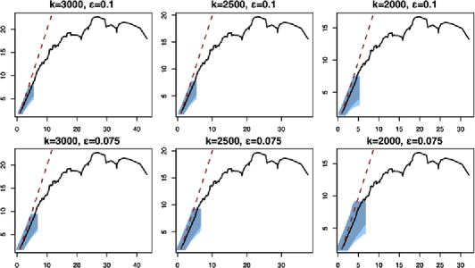
Figure 5: ME plot for 50,000 i.i.d. right-skewed stable random variables with $\xi=2/3$.

6.1.2 ME plots

Figure 4 shows the ME plot obtained from a data simulated from the Pareto distribution with $\xi=0.25$. The six plots correspond to different values of $k$ (3000, 2500 and 2000) and $\varepsilon$ (0.1 and 0.075). The black line is the observed ME plot, and the brown dotted line denotes the limit in probability. Again, the three shades of the colored bands denote the $99\%,95\%$ and the $90\%$ confidence bands for the plot, respectively. Note that the weak limit is a functional of the Brownian bridge and depends on $\xi$. We estimate $\xi$ using the Hill estimator and obtain the bounds by simulating 10,000 paths from the weak limit.

A striking feature in all these plots is that they are close to being linear near the bottom-left corner and become quite erratic near top-right corner. The reason behind this phenomenon is that the empirical ME function for high thresholds is the average of the excesses of a small number of upper order statistics. When averaging over few numbers, there is high variability, and therefore this part of the plot appears very nonlinear and is uninformative. Therefore, while obtaining confidence bands it is essential to leave out some of the extreme order statistics. We would also like to point out that, without the confidence bands, it would have been difficult to believe that these plots were obtained from a distribution with tail index $0.25$.

A simulation of ME plot for the right skewed stable distribution with $\xi=2/3$ is shown in Figure 5. We use the band described in (5.2.1) and estimate the quantiles using simulation. In this case we only provide the $95\%$ and the $90\%$ confidence band. The $99\%$ confidence band for the stable is very large and using that is not much helpful.

The next simulation is the ME plot for a sample from the distribution function described in (56), and the result is given in Figure 6. We use the same values for $n,k$ and $\varepsilon$. We see that this method of getting confidence bands works well in these cases.

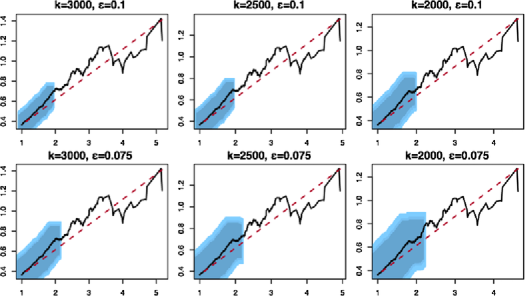
Figure 6: ME plot for 50,000 i.i.d. random variables with the distribution described in (56) ($\xi=0.2$).

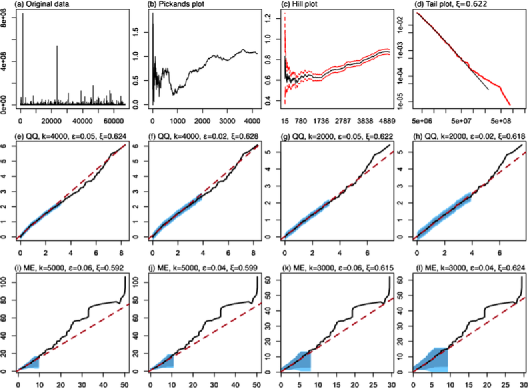
Figure 7: Analysis of the internet response size data.

6.2 An example with a real data

We study a data set which contains Internet response sizes corresponding to user requests. The sizes are thresholded to be at least 100 KB. The data set consists of 67,287 observations and is part of a bigger set collected in April 2000 at the University of North Carolina at Chapel Hill.

It is often stated that file size data typically exhibits heavy tails, and we observe that is indeed the case here. Figure 7 shows various plots from this data set. The sample variance is of the order of $10^{13}$ which suggests that the variance is possibly infinite for the underlying distribution (denote by $F$). This would imply that if $\bar{F}$ is regularly varying for some $\xi$, then we must have $\xi\geq 1/2$. This is suggested by both the Pickands plot and the Hill plot (Figure 7(b) and (c), resp.). The Hill plot is always above $1/2$ and the Pickands is above $1/2$ for most of the range. But it is difficult to get an estimate of $\xi$ using these two tools since both plots are highly fluctuating and hence inconclusive. We fit a GPD model with the top 2000 order statistics using the command “fit.GPD” in the library “QRMlib.” It gives an estimate $0.6218$ of $\xi$ and Figure 7(d) plots the estimated $\bar{F}$ in the log-log scale along with the fitted line.

We try the QQ plot with data set for $k=4000$ and $2000$ (top 6% and 3% order statistics approximately) and with $\varepsilon=0.05$ and $0.02$. The plots give an estimate of around 0.62 of $\xi$. The plots are shown in Figure 7(e)–(h). The ME plots for $k=5000,3000$ and $\varepsilon=0.06,0.04$ are shown in Figure 7(i)–(l), and they also suggest a similar estimate for $\xi$.

We observe that, in this example, the different methods of understanding the tail behavior of a data work very well, and all of them are in agreement about the value of $\xi$. This is not true in many situations, and then it is hard to judge which method one should trust. In those cases it is important to have some more knowledge about the system from which the data was collected, and often that helps in the understanding of the data.

7 Conclusion

Plotting techniques have always been popular as diagnostic tools for goodness-of-fit of observed data, and we believe they will remain so because of their visual and intuitive appeal. In this paper we have concentrated on two such tools used extensively in the extreme-value literature. A weak law of large numbers has been shown previously for both the QQ plots (Das and Resnick [9]) and ME plots (Ghosh and Resnick [22]), considering them as random elements in an appropriate topology. Our contribution in this paper has been to provide distributional limits for them. In the case of QQ plots, we have also provided an explicit expression for confidence bounds (with a truncation to avoid the confidence bounds from blowing up) by using these distributional results. In the case of ME plots we have obtained distributional limits in the cases $0<\xi<1/2$, $1/2<\xi<1$ and $\xi\geq 1$ separately where the underlying distribution $F$ is assumed to be regularly varying with index $-1/\xi$. The case $\xi=1/2$ is still open. We have produced confidence bounds for the ME plots in these cases by Monte Carlo simulation, as explicit expressions for these quantities are not easy to calculate. The explicit expressions would involve boundary-crossing probabilities for a Brownian Bridge with nonlinear boundaries. Boundary-crossing probabilities for Brownian motion can be approximated using piecewise linear boundaries Pötzelberger and Wang [31], but we do not know of a nice approximation for the Brownian Bridge case; hence we resort to simulation. We have illustrated the confidence bounds in both the cases of QQ plots and ME plots with simulated and real data examples in Section 6. The importance of the confidence bounds can be understood very clearly from Figure 4. Here we have a simulated data set of 50,000 points from a Pareto distribution with parameter $\xi=0.25$. Just looking at the ME plot, it is not at all obvious that this is a heavy-tailed data, whereas when the confidence bounds with the $\varepsilon$-truncation are drawn, the straight line with slope $\xi=0.25$ remains inside the bounds indicating the true nature of the data.

Since we are using the limiting distribution to obtain the confidence bounds, it is natural to ask what the rate of convergence is. We have observed that this method works well in the simulation studies that we have done, but we have not answered this theoretically. This is currently a work in progress.

A standing assumption in the results we proved in this paper is that the random variables $X_{n}$ are i.i.d. We believe that it is possible to obtain similar results under a more general assumption of stationarity and mixing; cf. Rootzén [35]. We intend to look into this further.

We should also note here that often practitioners use the median-excess plot with the implied meaning when $\xi>1$; that is, the mean for the distribution does not exist (Embrechts, Klüppelberg and Mikosch [18]), but we have not ventured into this kind of plotting tool. We have also not looked into other kinds of plots used in extremes, like the Stărică plot (Stărică [40]) to determine the right $k$ number of upper order statistics, or the Gertensgarbe and Werner plot (Gertensgarbe and Werner [21]), for determining thresholds, over which a data may be assumed to be extreme-valued, or the more popular Hill plot, Pickands plot (Resnick [33]), to detect the right value of the extreme-value parameter. Obtaining results in the same spirit as this paper for these other varieties of plots are a part of intended future research.

References

- [1] {barticle}[mr] \bauthor\bsnmBeer, \bfnmGerald\binitsG. (\byear1993). \btitleOn the Fell topology. \bjournalSet-Valued Anal. \bvolume1 \bpages69–80. \biddoi=10.1007/BF01039292, issn=0927-6947, mr=1230370 \bptokimsref \endbibitem
- [2] {bbook}[mr] \bauthor\bsnmBillingsley, \bfnmPatrick\binitsP. (\byear1968). \btitleConvergence of Probability Measures. \baddressNew York: \bpublisherWiley. \bidmr=0233396 \bptokimsref \endbibitem
- [3] {bbook}[mr] \bauthor\bsnmBingham, \bfnmN. H.\binitsN.H., \bauthor\bsnmGoldie, \bfnmC. M.\binitsC.M. &\bauthor\bsnmTeugels, \bfnmJ. L.\binitsJ.L. (\byear1987). \btitleRegular Variation. \bseriesEncyclopedia of Mathematics and Its Applications \bvolume27. \baddressCambridge: \bpublisherCambridge Univ. Press. \bidmr=0898871 \bptokimsref \endbibitem
- [4] {bmisc}[author] \bauthor\bsnmChow, \bfnmT. L.\binitsT.L. &\bauthor\bsnmTeugels, \bfnmJ. L.\binitsJ.L. (\byear1978). \bhowpublishedThe sum and the maximum of iid random variables. In Proceedings of the Second Prague Symposium on Asymptotic Statistics. Amsterdam: North-Holland. \bptokimsref \endbibitem
- [5] {barticle}[mr] \bauthor\bsnmCsörgő, \bfnmMiklós\binitsM. &\bauthor\bsnmMason, \bfnmDavid M.\binitsD.M. (\byear1985). \btitleOn the asymptotic distribution of weighted uniform empirical and quantile processes in the middle and on the tails. \bjournalStochastic Process. Appl. \bvolume21 \bpages119–132. \biddoi=10.1016/0304-4149(85)90381-3, issn=0304-4149, mr=0834992 \bptokimsref \endbibitem
- [6] {barticle}[mr] \bauthor\bsnmCsörgő, \bfnmSándor\binitsS., \bauthor\bsnmHaeusler, \bfnmErich\binitsE. &\bauthor\bsnmMason, \bfnmDavid M.\binitsD.M. (\byear1991). \btitleThe asymptotic distribution of extreme sums. \bjournalAnn. Probab. \bvolume19 \bpages783–811. \bidissn=0091-1798, mr=1106286 \bptokimsref \endbibitem
- [7] {barticle}[mr] \bauthor\bsnmCsörgő, \bfnmSándor\binitsS., \bauthor\bsnmHorváth, \bfnmLajos\binitsL. &\bauthor\bsnmMason, \bfnmDavid M.\binitsD.M. (\byear1986). \btitleWhat portion of the sample makes a partial sum asymptotically stable or normal? \bjournalProbab. Theory Relat. Fields \bvolume72 \bpages1–16. \biddoi=10.1007/BF00343893, issn=0178-8051, mr=0835156 \bptokimsref \endbibitem
- [8] {barticle}[mr] \bauthor\bsnmDarling, \bfnmD. A.\binitsD.A. (\byear1952). \btitleThe influence of the maximum term in the addition of independent random variables. \bjournalTrans. Amer. Math. Soc. \bvolume73 \bpages95–107. \bidissn=0002-9947, mr=0048726 \bptokimsref \endbibitem
- [9] {barticle}[mr] \bauthor\bsnmDas, \bfnmB.\binitsB. &\bauthor\bsnmResnick, \bfnmS. I.\binitsS.I. (\byear2008). \btitleQQ plots, random sets and data from a heavy tailed distribution. \bjournalStoch. Models \bvolume24 \bpages103–132. \biddoi=10.1080/15326340701828308, issn=1532-6349, mr=2384693 \bptokimsref \endbibitem
- [10] {barticle}[mr] \bauthor\bsnmD’Auria, \bfnmBernardo\binitsB. &\bauthor\bsnmResnick, \bfnmSidney I.\binitsS.I. (\byear2006). \btitleData network models of burstiness. \bjournalAdv. in Appl. Probab. \bvolume38 \bpages373–404. \biddoi=10.1239/aap/1151337076, issn=0001-8678, mr=2264949 \bptokimsref \endbibitem
- [11] {barticle}[mr] \bauthor\bsnmDavison, \bfnmA. C.\binitsA.C. &\bauthor\bsnmSmith, \bfnmR. L.\binitsR.L. (\byear1990). \btitleModels for exceedances over high thresholds (with discussion and a reply by the authors). \bjournalJ. Roy. Statist. Soc. Ser. B \bvolume52 \bpages393–442. \bidissn=0035-9246, mr=1086795 \bptnotecheck related \bptokimsref \endbibitem
- [12] {bbook}[mr] \bauthor\bparticlede \bsnmHaan, \bfnmL.\binitsL. (\byear1970). \btitleOn Regular Variation and Its Application to the Weak Convergence of Sample Extremes. \bseriesMathematical Centre Tracts \bvolume32. \baddressAmsterdam: \bpublisherMathematisch Centrum. \bidmr=0286156 \bptnotecheck related \bptokimsref \endbibitem
- [13] {bbook}[mr] \bauthor\bparticlede \bsnmHaan, \bfnmLaurens\binitsL. &\bauthor\bsnmFerreira, \bfnmAna\binitsA. (\byear2006). \btitleExtreme Value Theory: An Introduction. \bseriesSpringer Series in Operations Research and Financial Engineering. \baddressNew York: \bpublisherSpringer. \bidmr=2234156 \bptokimsref \endbibitem
- [14] {barticle}[mr] \bauthor\bparticlede \bsnmHaan, \bfnmL.\binitsL. &\bauthor\bsnmPeng, \bfnmL.\binitsL. (\byear1998). \btitleComparison of tail index estimators. \bjournalStatist. Neerlandica \bvolume52 \bpages60–70. \biddoi=10.1111/1467-9574.00068, issn=0039-0402, mr=1615558 \bptokimsref \endbibitem
- [15] {barticle}[mr] \bauthor\bparticlede \bsnmHaan, \bfnmLaurens\binitsL. &\bauthor\bsnmStadtmüller, \bfnmUlrich\binitsU. (\byear1996). \btitleGeneralized regular variation of second order. \bjournalJ. Austral. Math. Soc. Ser. A \bvolume61 \bpages381–395. \bidissn=0263-6115, mr=1420345 \bptokimsref \endbibitem
- [16] {barticle}[mr] \bauthor\bsnmDoob, \bfnmJ. L.\binitsJ.L. (\byear1949). \btitleHeuristic approach to the Kolmogorov–Smirnov theorems. \bjournalAnn. Math. Statistics \bvolume20 \bpages393–403. \bidissn=0003-4851, mr=0030732 \bptokimsref \endbibitem
- [17] {barticle}[author] \bauthor\bsnmDrees, \bfnmH.\binitsH. (\byear2011). \btitleExtreme value analysis of actuarial risks: Estimation and model validation. Available at http://arxiv.org/abs/1103.2872. \bptokimsref \endbibitem
- [18] {bbook}[mr] \bauthor\bsnmEmbrechts, \bfnmPaul\binitsP., \bauthor\bsnmKlüppelberg, \bfnmClaudia\binitsC. &\bauthor\bsnmMikosch, \bfnmThomas\binitsT. (\byear1997). \btitleModelling Extremal Events for Insurance and Finance. \bseriesApplications of Mathematics (New York) \bvolume33. \baddressBerlin: \bpublisherSpringer. \bidmr=1458613 \bptokimsref \endbibitem
- [19] {barticle}[mr] \bauthor\bsnmFlachsmeyer, \bfnmJürgen\binitsJ. (\byear1963). \btitleVerschiedene Topologisierungen im Raum der abgeschlossenen Mengen. \bjournalMath. Nachr. \bvolume26 \bpages321–337. \bidissn=0025-584X, mr=0174026 \bptnotecheck year \bptokimsref \endbibitem
- [20] {bbook}[mr] \bauthor\bsnmGeluk, \bfnmJ. L.\binitsJ.L. &\bauthor\bparticlede \bsnmHaan, \bfnmL.\binitsL. (\byear1987). \btitleRegular Variation, Extensions and Tauberian Theorems. \bseriesCWI Tract \bvolume40. \baddressAmsterdam: \bpublisherStichting Mathematisch Centrum, Centrum voor Wiskunde en Informatica. \bidmr=0906871 \bptokimsref \endbibitem
- [21] {barticle}[author] \bauthor\bsnmGertensgarbe, \bfnmF. W.\binitsF.W. &\bauthor\bsnmWerner, \bfnmP. C.\binitsP.C. (\byear1989). \btitleA method for the statistical definition of extreme-value regions and their application to meteorological time series. \bjournalZeitschrift für Meteorologie \bvolume39 \bpages224–226. \bptokimsref \endbibitem
- [22] {barticle}[mr] \bauthor\bsnmGhosh, \bfnmSouvik\binitsS. &\bauthor\bsnmResnick, \bfnmSidney\binitsS. (\byear2010). \btitleA discussion on mean excess plots. \bjournalStochastic Process. Appl. \bvolume120 \bpages1492–1517. \biddoi=10.1016/j.spa.2010.04.002, issn=0304-4149, mr=2653263 \bptokimsref \endbibitem
- [23] {bbook}[mr] \bauthor\bsnmHogg, \bfnmRobert V.\binitsR.V. &\bauthor\bsnmKlugman, \bfnmStuart A.\binitsS.A. (\byear1984). \btitleLoss Distributions. \bseriesWiley Series in Probability and Mathematical Statistics: Applied Probability and Statistics. \baddressNew York: \bpublisherWiley. \biddoi=10.1002/9780470316634, mr=0747141 \bptokimsref \endbibitem
- [24] {barticle}[author] \bauthor\bsnmKatz, \bfnmR. W.\binitsR.W., \bauthor\bsnmParlange, \bfnmM. B.\binitsM.B. &\bauthor\bsnmNaveau, \bfnmP.\binitsP. (\byear2002). \btitleStatistics of extremes in hydrology. \bjournalAdvances in Water Resources \bvolume25 \bpages1287–1304. \bptokimsref \endbibitem
- [25] {barticle}[mr] \bauthor\bsnmKratz, \bfnmMarie\binitsM. &\bauthor\bsnmResnick, \bfnmSidney I.\binitsS.I. (\byear1996). \btitleThe -estimator and heavy tails. \bjournalComm. Statist. Stochastic Models \bvolume12 \bpages699–724. \biddoi=10.1080/15326349608807407, issn=0882-0287, mr=1410853 \bptokimsref \endbibitem
- [26] {bbook}[mr] \bauthor\bsnmMatheron, \bfnmG.\binitsG. (\byear1975). \btitleRandom Sets and Integral Geometry. \bseriesWiley Series in Probability and Mathematical Statistics. \baddressNew York–London–Sydney: \bpublisherWiley. \bidmr=0385969 \bptokimsref \endbibitem
- [27] {barticle}[mr] \bauthor\bsnmMaulik, \bfnmKrishanu\binitsK., \bauthor\bsnmResnick, \bfnmSidney\binitsS. &\bauthor\bsnmRootzén, \bfnmHolger\binitsH. (\byear2002). \btitleAsymptotic independence and a network traffic model. \bjournalJ. Appl. Probab. \bvolume39 \bpages671–699. \bidissn=0021-9002, mr=1938164 \bptokimsref \endbibitem
- [28] {bbook}[mr] \bauthor\bsnmMcNeil, \bfnmAlexander J.\binitsA.J., \bauthor\bsnmFrey, \bfnmRüdiger\binitsR. &\bauthor\bsnmEmbrechts, \bfnmPaul\binitsP. (\byear2005). \btitleQuantitative Risk Management: Concepts, Techniques and Tools. \bseriesPrinceton Series in Finance. \baddressPrinceton, NJ: \bpublisherPrinceton Univ. Press. \bidmr=2175089 \bptokimsref \endbibitem
- [29] {bbook}[mr] \bauthor\bsnmMolchanov, \bfnmIlya\binitsI. (\byear2005). \btitleTheory of Random Sets. \bseriesProbability and Its Applications (New York). \baddressLondon: \bpublisherSpringer. \bidmr=2132405 \bptokimsref \endbibitem
- [30] {bbook}[mr] \bauthor\bsnmØksendal, \bfnmBernt\binitsB. (\byear2003). \btitleStochastic Differential Equations: An Introduction with Applications, \bedition6th ed. \bseriesUniversitext. \baddressBerlin: \bpublisherSpringer. \bidmr=2001996 \bptokimsref \endbibitem
- [31] {barticle}[mr] \bauthor\bsnmPötzelberger, \bfnmKlaus\binitsK. &\bauthor\bsnmWang, \bfnmLiqun\binitsL. (\byear2001). \btitleBoundary crossing probability for Brownian motion. \bjournalJ. Appl. Probab. \bvolume38 \bpages152–164. \bidissn=0021-9002, mr=1816120 \bptokimsref \endbibitem
- [32] {barticle}[mr] \bauthor\bsnmResnick, \bfnmSidney I.\binitsS.I. (\byear1986). \btitlePoint processes, regular variation and weak convergence. \bjournalAdv. in Appl. Probab. \bvolume18 \bpages66–138. \biddoi=10.2307/1427239, issn=0001-8678, mr=0827332 \bptokimsref \endbibitem
- [33] {bbook}[mr] \bauthor\bsnmResnick, \bfnmSidney I.\binitsS.I. (\byear2007). \btitleHeavy-Tail Phenomena: Probabilistic and Statistical Modeling. \bseriesSpringer Series in Operations Research and Financial Engineering. \baddressNew York: \bpublisherSpringer. \bidmr=2271424 \bptokimsref \endbibitem
- [34] {bbook}[mr] \bauthor\bsnmResnick, \bfnmSidney I.\binitsS.I. (\byear2008). \btitleExtreme Values, Regular Variation and Point Processes. \bseriesSpringer Series in Operations Research and Financial Engineering. \baddressNew York: \bpublisherSpringer. \bnoteReprint of the 1987 original. \bidmr=2364939 \bptokimsref \endbibitem
- [35] {barticle}[mr] \bauthor\bsnmRootzén, \bfnmHolger\binitsH. (\byear2009). \btitleWeak convergence of the tail empirical process for dependent sequences. \bjournalStochastic Process. Appl. \bvolume119 \bpages468–490. \biddoi=10.1016/j.spa.2008.03.003, issn=0304-4149, mr=2494000 \bptokimsref \endbibitem
- [36] {barticle}[mr] \bauthor\bsnmRossberg, \bfnmHans-Joachim\binitsH.J. (\byear1967). \btitleÜber das asymptotische Verhalten der Rand- und Zentralglieder einer Variationsreihe. II. \bjournalPubl. Math. Debrecen \bvolume14 \bpages83–90. \bidissn=0033-3883, mr=0225454 \bptokimsref \endbibitem
- [37] {bbook}[mr] \bauthor\bsnmSeneta, \bfnmEugene\binitsE. (\byear1976). \btitleRegularly Varying Functions. \bseriesLecture Notes in Mathematics \bvolume508. \baddressBerlin: \bpublisherSpringer. \bidmr=0453936 \bptokimsref \endbibitem
- [38] {bbook}[mr] \bauthor\bsnmShorack, \bfnmGalen R.\binitsG.R. &\bauthor\bsnmWellner, \bfnmJon A.\binitsJ.A. (\byear1986). \btitleEmpirical Processes with Applications to Statistics. \bseriesWiley Series in Probability and Mathematical Statistics: Probability and Mathematical Statistics. \baddressNew York: \bpublisherWiley. \bidmr=0838963 \bptokimsref \endbibitem
- [39] {bincollection}[author] \bauthor\bsnmSmith, \bfnmR. L.\binitsR.L. (\byear2003). \btitleStatistics of extremes, with applications in environment, insurance and finance. In \bbooktitleSemStat: Seminaire Europeen de Statistique, Exteme Values in Finance, Telecommunications, and the Environment (\beditor\bfnmB.\binitsB. \bsnmFinkenstadt &\beditor\bfnmH.\binitsH. \bsnmRootzén, eds.) \bpages1–78. \baddressLondon: \bpublisherChapman & Hall. \bptokimsref \endbibitem
- [40] {barticle}[author] \bauthor\bsnmStărică, \bfnmC.\binitsC. (\byear1999). \btitleMultivariate extremes for models with constant conditional correlations. \bjournalJournal of Empirical Finance \bvolume6 \bpages515–553. \bptokimsref \endbibitem
- [41] {bbook}[mr] \bauthor\bparticlevan der \bsnmVaart, \bfnmAad W.\binitsA.W. &\bauthor\bsnmWellner, \bfnmJon A.\binitsJ.A. (\byear1996). \btitleWeak Convergence and Empirical Processes with Applications to Statistics. \bseriesSpringer Series in Statistics. \baddressNew York: \bpublisherSpringer. \bidmr=1385671 \bptokimsref \endbibitem
- [42] {bincollection}[mr] \bauthor\bsnmVervaat, \bfnmWim\binitsW. (\byear1997). \btitleRandom upper semicontinuous functions and extremal processes. In \bbooktitleProbability and Lattices. \bseriesCWI Tract \bvolume110 \bpages1–56. \baddressAmsterdam: \bpublisherMath. Centrum Centrum Wisk. Inform. \bidmr=1465481 \bptokimsref \endbibitem
- [43] {barticle}[mr] \bauthor\bsnmYang, \bfnmGrace L.\binitsG.L. (\byear1978). \btitleEstimation of a biometric function. \bjournalAnn. Statist. \bvolume6 \bpages112–116. \bidissn=0090-5364, mr=0471233 \bptokimsref \endbibitem