On the Orchard crossing number of complete bipartite graphs

Abstract.

We compute the Orchard crossing number, which is defined in a similar way to the rectilinear crossing number, for the complete bipartite graphs $K_{n,n}$.

1. Introduction

Let $G$ be an abstract graph. Motivated by the Orchard relation, introduced in [3, 4], we have defined the Orchard crossing number of $G$ [5], in a similar way to the well-known rectilinear crossing number of an abstract graph $G$ (denoted by $\overline{\rm cr}(G)$, see [1, 8]). A general reference for crossing numbers can be [6].

The Orchard crossing number is interesting for several reasons. First, it is based on the Orchard relation which is an equivalence relation on the vertices of a graph, with at most two equivalence classes (see [3]). Moreover, since the Orchard relation can be defined for higher dimensions too (see [3]), hence the Orchard crossing number may be also generalized to higher dimensions.

Second, a variant of this crossing number is tightly connected to the well-known rectilinear crossing number (see Proposition 2.5 below).

Third, one can find real problems which the Orchard crossing number can represent. For example, design a network of computers which should be constructed in a manner which allows possible extensions of the network in the future. Since we want to avoid (even future) crossings of the cables which are connecting between the computers, we need to count not only the present crossings, but also the separators (which might come to cross in the future).

In this paper, we compute the Orchard crossing number for the complete bipartite graphs $K_{n,n}$:

Theorem 1.1.

$${\rm OCN}(K_{n,n})=4n{n\choose 3}$$

This value is attained where all the $2n$ points are in a convex position and alternate in color (see Figure 1 for an example for $n=4$).

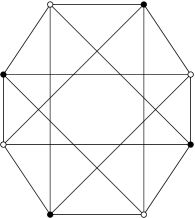
Figure 1. The optimal rectilinear drawing for ${\rm OCN}(K_{4,4})$

The ideas of the proof are quite similar to those of [2], where the maximal value of the maximum rectilinear crossing number has been computed for some families of graphs, but still are not straightforward from them. This again shows the tight connection between the Orchard crossing number and the rectilinear crossing number.

The proof is based on two parts: in the first part, we show that the optimal drawing of $K_{n,n}$, presented in Figure 1 for $n=4$, has $4n{n\choose 3}$ Orchard crossings, and hence ${\rm OCN}(K_{n,n})\leq 4n{n\choose 3}$ (see Section 3). In the second part, we show that any drawing of $K_{n,n}$ has at least $4n{n\choose 3}$ Orchard crossings, so ${\rm OCN}(K_{n,n})\geq 4n{n\choose 3}$ (see Section 4).

The paper is organized as follows. In Section 2, we present the Orchard relation, define the Orchard crossing number, and give some examples. Sections 3 and 4 contain the two parts of the proof of Theorem 1.1.

2. The Orchard crossing numbers

We start with some notations. A finite set $\mathcal{P}=\{P_{1},\dots,P_{n}\}$ of $n$ points in the plane $\mathbb{R}^{2}$ is a generic configuration if no three points of $\mathcal{P}$ are collinear.

A line $L\subset\mathbb{R}^{2}$ separates two points $P,Q\in(\mathbb{R}^{2}\setminus L)$ if $P$ and $Q$ are in different connected components of $\mathbb{R}^{2}\setminus L$. Given a generic configuration $\mathcal{P}$, denote by $n(P,Q)$ the number of lines defined by pairs of points in $\mathcal{P}\setminus\{P,Q\}$, which separate $P$ and $Q$.

For defining the Orchard crossing number of an abstract graph $G$, we need some more notions.

Definition 2.1 (Rectilinear drawing of an abstract graph $G$).

Let $G=(V,E)$ be an abstract graph, where $V$ is its set of vertices and $E$ is its set of edges. A rectilinear drawing of the abstract graph $G$, denoted by $R(G)$, is a generic configuration of points $V^{\prime}$ in the affine plane, in bijection with $V$. An edge $(s,t)\in E$ is represented by the straight segment $[s^{\prime},t^{\prime}]$ in $\mathbb{R}^{2}$.

Then, we associate a crossing number to such a drawing:

Definition 2.2.

Let $R(G)$ be a rectilinear drawing of the abstract graph $G=(V,E)$. The crossing number of $R(G)$, denoted by $n(R(G))$, is:

$$n(R(G))=\sum_{(s,t)\in E}n(s,t)$$

Note that the sum is taken only over the edges of the graph, whence $n(s,t)$ counts in all the lines generated by pairs of points of the configuration.

Now, we can define the Orchard crossing number of an abstract graph $G=(V,E)$:

Definition 2.3 (Orchard crossing number).

Let $G=(V,E)$ be an abstract graph. The Orchard crossing number of $G$, denoted by ${\rm OCN}(G)$, is

$${\rm OCN}(G)=\min_{R(G)}(n(R(G)))$$

A variant of the Orchard crossing number is the maximal Orchard crossing number:

Definition 2.4 (Maximal Orchard crossing number).

Let $G=(V,E)$ be an abstract graph. The maximal Orchard crossing number of $G$, denoted by ${\rm MOCN}(G)$, is

$${\rm MOCN}(G)=\max_{R(G)}(n(R(G)))$$

This variant is extremely interesting due to the following result (see [5, Proposition 2.7]):

Proposition 2.5.

The rectilinear drawing which yields the maximal Orchard crossing number for complete graphs $K_{n}$ is the same as the rectilinear drawing which attains the rectilinear crossing number of $K_{n}$.

The importance of this result is that it might be possible that the computation of the maximal Orchard crossing number will be easier than the computation of the rectilinear crossing number.

3. An upper bound for ${\rm OCN}(K_{n,n})$

In this section, we show the easy part of Theorem 1.1 by proving that the mentioned value $4n{n\choose 3}$ is indeed attained by the rectilinear drawing of $K_{n,n}$, where all the $2n$ points are in a convex position and alternate in color (see Figure 1 for $n=4$).

Lemma 3.1.

Assume that $R(K_{n,n})$ is the rectilinear drawing of $K_{n,n}$ which realizes the $2n$ points of $K_{n,n}$ as the points of a regular $2n$-gon, and the points change colors alternately. Then:

$$n(R(K_{n,n}))=4n{n\choose 3}$$

Proof.

Since any quadruple of points is in a convex position, we have to consider only four types of quadruples:

1. All the points of the quadruple have the same color. This case contributes nothing to the number of crossings (see Figure 2(a)).

2. The quadruple consists of two black points and two white points, and the points change colors alternately. This case contributes nothing to the number of crossings (see Figure 2(b), where the solid lines are edges of the graph and the dashed lines are lines generated by a pair of points of the same color which are not edges of the graph).

3. Three of the points are black and one point is white (or vice versa). This case contributes $1$ to the number of crossings (see Figure 2(c)).

4. The quadruple consists of two consecutive black points followed by two consecutive white points. This case contributes $2$ to the number of crossings (see Figure 2(d)).

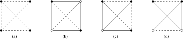
Figure 2. Four cases of quadruples of points in a convex position

Hence, we have to compute the number of quadruples of types (3) and (4) respectively, and to multiply these numbers by their corresponding contributions to the total number of crossings.

Assume that we have $n$ white points and $n$ black points. For computing the number of quadruples of type (3), we have to choose three black points out of $n$ black points, and then to choose one point out of $n$ white points. There are $n{n\choose 3}$ possibilities to do so. Since, we have to do the same with the opposite colors, we have $2n{n\choose 3}$ quadruples of type (3), which contribute $2n{n\choose 3}$ to the total number of crossings.

The count of quadruples of type (4) is a bit more complicated. We count them in the following way: Choose an arbitrary point. Then choose another point of the same color. Then, choose two points of the opposite color to the left of the second point, but to the right of the first point. One can easily see that the number of possibilities is:

$$\frac{2n}{4}\sum_{k=2}^{n-1}k(k-1),$$

where the sum is induced from choosing the second point of the first color. The division by $4$ comes from the fact that by this counting argument, each quadruple is counted $4$ times, once for each point of it.

We simplify this expression:

$$\frac{2n}{4}\sum_{k=2}^{n-1}k(k-1) = \frac{n}{2}\sum_{k=1}^{n-1}(k^{2}-k)=$$

$$= \frac{n}{2}\left(\frac{(n-1)n(2n-1)}{6}-\frac{n(n-1)}{2}\right)=$$

$$= \frac{n\cdot n(n-1)(n-2)}{6}=n{n\choose 3}$$

Hence, we get that the number of quadruples of type (4) is $n{n\choose 3}$. Since each quadruple of type (4) contributes two crossings, this number should be multiplied by $2$ for getting the total contribution of the quadruples of type (4). Hence, the quadruples of type (4) contribute $2n{n\choose 3}$.

Summing up the two contributions yields the result. ∎

4. A lower bound for ${\rm OCN}(K_{n,n})$

In this section, we show the difficult part of Theorem 1.1 by proving that for any rectilinear drawing of $K_{n,n}$ there are at least $4n{n\choose 3}$ Orchard crossings. This will show that $4n{n\choose 3}$ is indeed a lower bound for ${\rm OCN}(K_{n,n})$.

The idea of proof is counting separately the Orchard crossings induced by pairs of points with different colors and by pairs of points with the same color (see Sections 4.1 and 4.2 respectively).

Together with the result of the previous section, this will prove Theorem 1.1 (see Section 4.3).

We start with one notation. A bw-pair is a pair of points consists of a black point and a white point.

4.1. Orchard crossings induced by lines generated by pairs of points with different colors

Let $D$ be a configuration of $n$ white points and $n$ black points. For each $k=1,2,\dots,n^{2}$, let $\ell_{k}$ be a line determined by a white point and a black point. For each $\ell_{k}$, let $a_{k}$ be the number of bw-pairs with one point in one halfplane determined by $\ell_{k}$, and the other point in the other halfplane. Let $A=\sum\limits_{k=1}^{n^{2}}a_{k}$.

Proposition 4.1.

$$A\geq 2n{n\choose 3}$$

Proof.

For each $\ell_{k}$, a black (resp. white) endvertex will be of type $i$ if the edge incident to $\ell_{k}$ divides the graph into two halfplanes, one contains $i$ black (resp. white) vertices, and the other contains $n-i-1$ black (resp. white) vertices. By symmetry, we only have to consider $0\leq i\leq\lfloor\frac{n-1}{2}\rfloor=N$. Let $y_{i}$ be the number of endvertices of type $i$. Thus, we have:

$$y_{0}+y_{1}+\cdots+y_{N}=2n^{2},$$

since we have $n^{2}$ such edges and each one is counted twice (for the white vertex and for the black vertex).

An edge which connects black and white vertices is of type $i,j$ if one halfplane determined by that edge has $i$ vertices of one color and $j$ vertices of the other color. Let $x_{i,j}$ be the number of edges of type $i,j$. By symmetry, we can assume that $0\leq i\leq j\leq N$ (we will justify this assumption later on). Note that $x_{i,j}=x_{j,i}$.

Thus, $y_{i}$ is related to $x_{i,j}$ by the following equation:

(1) $$y_{i}=2x_{i,i}+\displaystyle\sum_{j=0}^{i-1}x_{j,i}+\displaystyle\sum_{j=i+1}^{N}x_{i,j},$$

due to the following argument: for being counted in $y_{i}$, an edge should have $i$ vertices of one color in one of the halfplanes it determines. The only case which is counted twice is when $i=j$, where it is counted for both colors.

Now, for an edge of type $i,j$, there are $i(n-j-1)+j(n-i-1)$ bw-pairs in opposite halfplanes of that edge. Summing it over all edges of a drawing, we obtain

$$M=\displaystyle\sum_{i=0}^{N}\displaystyle\sum_{j=i}^{N}\left[i(n-j-1)+j(n-i-1)\right]x_{i,j}$$

bw-pairs in opposite halfplanes. We are looking for a drawing which minimizes $M$.

We now justify our assumption that $0\leq i\leq j\leq N$, where $i$ and $j$ are the number of vertices of the two colors in the same halfplane of an edge. Assume that for a given type $i,j$ edge, the $i$ vertices of one color and the $j$ vertices of the other color are in different halfplanes. This yields $ij+(n-j-1)(n-i-1)$ bw-pairs. However,

$$i(n-j-1)+j(n-i-1)\leq ij+(n-j-1)(n-i-1)$$

for $0\leq i\leq j\leq N$. Hence our assumption reduces the number of bw-pairs.

In order to minimize $M$, we start by multiplying Equation (1) by $i(n-i-1)$, and subtracting it from $M$ for all values of $i$, yielding:

$$M-\displaystyle\sum_{i=1}^{N}i(n-i-1)y_{i}=$$

$$= \displaystyle\sum_{i=0}^{N}\displaystyle\sum_{j=i}^{N}\left[i(n-j-1)+j(n-i-1)\right]x_{i,j}$$

$$\qquad-\displaystyle\sum_{i=1}^{N}i(n-i-1)\left(2x_{i,i}+\displaystyle\sum_{j=0}^{i-1}x_{j,i}+\displaystyle\sum_{j=i+1}^{N}x_{i,j}\right)=$$

$$= \displaystyle\sum_{i=0}^{N}\displaystyle\sum_{j=i+1}^{N}\left[i(n-j-1)+j(n-i-1)\right]x_{i,j}$$

$$\qquad-\displaystyle\sum_{i=1}^{N}i(n-i-1)\left(\displaystyle\sum_{j=0}^{i-1}x_{j,i}+\displaystyle\sum_{j=i+1}^{N}x_{i,j}\right)=$$

$$= \displaystyle\sum_{i=0}^{N}\displaystyle\sum_{j=i+1}^{N}\left[i(i-j)+j(n-i-1)\right]x_{i,j}$$

$$\qquad-\sum_{i=0}^{N-1}\sum_{j=i+1}^{N}j(n-j-1)x_{i,j}=$$

$$= \displaystyle\sum_{i=0}^{N}\displaystyle\sum_{j=i+1}^{N}\left[i(i-j)+j(j-i)\right]x_{i,j}=\displaystyle\sum_{i=0}^{N-1}\displaystyle\sum_{j=i+1}^{N}(j-i)^{2}x_{i,j}$$

Hence, we have:

(2) $$M=\displaystyle\sum_{i=1}^{N}i(n-i-1)y_{i}+\displaystyle\sum_{i=0}^{N-1}\displaystyle\sum_{j=i+1}^{N}(j-i)^{2}x_{i,j}$$

For the next step, we introduce a new notation $p_{s,t}$. We first motivate it. Note that every white (resp. black) vertex $v_{i}$ serves as an endvertex for $n$ edges of the graph. For each of these $n$ edges, let $c_{i,j}$ ($1\leq j\leq n$) be the number of black (resp. white) points in the halfplane with a smaller number of black (resp. white) points determined by this edge. Thus, for each $v_{i}$, we have a sequence of $n$ numbers $(c_{i,1},\dots,c_{i,n})$ representing the types which $v_{i}$ is for the $n$ edges connected to $v_{i}$.

For example, for a white point $v$ on the convex hull of an alternating $2n$-gon (see Figure 3 for $n=4$, where only some of the edges are drawn), the two edges going to the adjacent black points (the edges $e_{1},e_{4}$) are of type $0$. The next two edges (edges $e_{2},e_{3}$) will be of type $1$, the next two edges (do not exist in this configuration) will be of type $2$, etc. Note that in this case we will have the same sequence of types for any point on the convex hull.

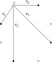
Figure 3. An example for computing $p_{s,t}$

Let $p_{s,t}$ be the number of white (resp. black) vertices having

$$s=\min\{c_{i,1},\dots,c_{i,n}\},$$

and the index $t$ is the number of distinct sorted sequences generated by all the vertices. For example, for the $2n$-gon configuration, we have $p_{0,1}=2n$, since all $2n$ vertices have $0$ as the lowest term in the sequence $0,0,1,1,2,2,\dots$. Note that there is a unique sequence for all the vertices. Therefore, $p_{0,t}=0$ for $t\geq 2$, since there is no vertex whose lowest type is $0$ which has a different sequence. Moreover, $p_{s,t}=0$ for $s\geq 1$, since there is no sequence whose lowest term is greater than $0$.

Since $p_{s,t}$ counts number of vertices, and in total there are $2n$ vertices, we have:

$$\sum_{s=0}^{N}\displaystyle\sum_{t\geq 1}p_{s,t}=2n.$$

Denote by $z_{s,t,i}$ the number of appearances of $i$ in the $t$th sequence whose lowest term is $s$. For example, assume that the first sequence is $0,1,2,1,0$. Then: $z_{0,1,0}=2$ because $0$ appears twice in the sequence. Similarly, $z_{0,1,1}=2$ since $1$ appears twice and $z_{0,1,2}=1$ since $2$ appears once.

It follows that:

(3) $$y_{i}=\displaystyle\sum_{t\geq 1}\displaystyle\sum_{s=0}^{i}z_{s,t,i}p_{s,t}$$

Additionally, since every vertex has $n$ edges, for fixed $s$ and $t$ we have that

(4) $$\sum_{i=s}^{N}z_{s,t,i}=n.$$

Since $\displaystyle\sum_{t\geq 1}\sum_{s=0}^{N}p_{s,t}=2n$, we obtain by Equation (3):

(5) $$y_{i}=4n+\displaystyle\sum_{t\geq 1}\left[\displaystyle\sum_{s=0}^{i}(z_{s,t,i}-2)p_{s,t}-2\displaystyle\sum_{s=i+1}^{N}p_{s,t}\right].$$

Respectively, for odd $n$, we have:

(6) $$y_{N}=2n+\displaystyle\sum_{t\geq 1}\displaystyle\sum_{s=0}^{N}(z_{s,t,N}-1)p_{s,t}.$$

We continue for even $n$. Using Equation (5), we can rewrite the first part of the expression for $M$ (Equation (2)) as follows:

$$\sum_{i=1}^{N}i(n-i-1)y_{i} = 4n\sum_{i=1}^{N}i(n-i-1)+$$

$$+\sum_{t\geq 1}\sum_{i=1}^{N}i(n-i-1)\left[\sum_{s=0}^{i}(z_{s,t,i}-2)p_{s,t}-2\sum_{s=i+1}^{N}p_{s,t}\right]$$

Following a change in the indices of the sums, this can be rewritten as:

$$4n\displaystyle\sum_{i=1}^{N}i(n-i-1)+\displaystyle\sum_{t\geq 1}\displaystyle\sum_{s=0}^{N}p_{s,t}\left[\displaystyle\sum_{i=s}^{N}i(n-i-1)(z_{s,t,i}-2)-2\displaystyle\sum_{i=1}^{s-1}i(n-i-1)\right]$$

This can again be rewritten as:

$$4n\sum_{i=1}^{N}i(n-i-1)+\left.\sum_{t\geq 1}\sum_{s=0}^{N}p_{s,t}\right[s(n-s-1)(z_{s,t,s}-2)+$$

$$\quad\left.+\sum_{i=s+1}^{N}i(n-i-1)(z_{s,t,i}-2)-2\sum_{i=1}^{s-1}i(n-i-1)\right]=$$

$$= 4n\sum_{i=1}^{N}i(n-i-1)+\sum_{t\geq 1}\sum_{s=0}^{N}p_{s,t}\left[s(n-s-1)\sum_{i=s}^{N}(z_{s,t,i}-2)+\right.$$

$$+\left.\displaystyle\sum_{i=s+1}^{N}[i(n-i-1)-s(n-s-1)](z_{s,t,i}-2)-2\displaystyle\sum_{i=1}^{s-1}i(n-i-1)\right]$$

Using Equation (4), it follows that this is also equal to:

$$4n\sum_{i=1}^{N}i(n-i-1)+\left.\sum_{t\geq 1}\sum_{s=0}^{N}p_{s,t}\right[C(s,n)+$$

$$\quad+\left.\sum_{i=s+1}^{N}[i(n-i-1)-s(n-s-1)](z_{s,t,i}-2)\right],$$

where

$$C(s,n) = s(n-s-1)(n-\displaystyle\sum_{i=s}^{N}2)-2\displaystyle\sum_{i=1}^{s-1}i(n-i-1)=$$

$$= s(n-s-1)(n-2(N-s+1))-2\displaystyle\sum_{i=1}^{s-1}i(n-i-1)$$

Now, we show that $C(s,n)$ is non-negative for all $0\leq s\leq N$ and $n$. For the proof, we will use the following observation:

Observation 4.2.

Let $a,b$ be such that: $0<a<b<\frac{n}{2}$. Then:

$$a(n-a)<b(n-b)$$

Lemma 4.3.

For all $0\leq s\leq N$ and $n$, $C(s,n)\geq 0$.

Proof.

By the definition of $N=\lfloor\frac{n-1}{2}\rfloor$, we have:

$$s(n-s-1)(n-2(N-s+1))\geq s(n-s-1)(2s-1).$$

Moreover, by Observation 4.2,

$$2\displaystyle\sum_{i=1}^{s-1}i(n-i-1) \leq 2\displaystyle\sum_{i=1}^{s-1}(s-1)(n-s)=$$

$$= 2(s-1)^{2}(n-s)$$

$$< s(n-s-1)(2s-2).$$

Therefore,

$$C(s,n)>s(n-s-1)(2s-1)-s(n-s-1)(2s-2)=s(n-s-1)\geq 0.$$

∎

We now show that $z_{s,t,i}-2\geq 0$. Since the term $z_{s,t,i}-1$ must be carried throughout this summation, the expression for odd $n$ is also minimized for $p_{s,t}=0$ for all $s\geq 1$, provided $z_{s,t,N}-1\geq 0$.

Lemma 4.4.

$z_{s,t,i}\geq 2$ for all $s,t,i$ such that $i>s$ and $z_{s,t,N}\geq 1$ for odd $n$.

Proof.

Without loss of generality, consider a given black vertex. We start by proving that there is at least one endvertex of type $\frac{n-1}{2}$ for odd $n$, and at least two endvertices of type $\frac{n-2}{2}$ for even $n$. This statement can be proved by induction on $n$. This statement is obvious for $n=2$ and $n=3$, so we start with the inductive step. Also, note that in traversing the $n$ edges incident to the given vertex in a clockwise or counterclockwise manner, in moving from edge to edge, the number of white vertices in the clockwise following halfplane may be changed by at most $1$. This fact will be used numerous times throughout the proof. We illustrate it by the following example:

Example 4.5.

Given a rectilinear drawing of $K_{4,4}$ at Figure 4 (where only some of edges are drawn). If we are traversing clockwise the $4$ edges starting frow the lowest black point, we have that the type of the edge $e_{1}$ is $0$, since there is no white point in the left halfplane defined by this edge. Next, the type of $e_{2}$ is $1$, since there is only one white point in the left halfplane defined by this edge. The type of $e_{3}$ is again $1$, since there is only one white point in the right halfplane defined by this edge. Finally, the type of $e_{4}$ is $0$, since there is no white point in the right halfplane defined by this edge.

Hence, we have that while moving from edge to edge, the number of white vertices in the clockwise following halfplane may be changed by at most $1$. Consequently, the types of the corresponding edges may be changed by at most $1$.

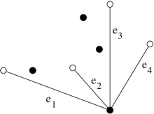
Figure 4. An example

Case I: Passing from odd $n$ to $n+1$.
Consider the edge for which this endvertex is of type $\frac{n-1}{2}$ in the configuration of $n$ white vertices and $n$ black vertices. When the $(n+1)$st pair of vertices is added, this original endvertex will be the first endvertex of type $\frac{(n+1)-2}{2}$. If the $(n+1)$st white vertex is added in this edge’s clockwise following halfplane, then an immediately following edge or edge extension has an endvertex of type $\frac{(n+1)-2}{2}$. Thus, either this edge or the edge corresponding to this extension will have the second endvertex of type $\frac{n-1}{2}$.

Case II: Passing from even $n$ to $n+1$.
Consider an edge with an endvertex of type $\frac{n-2}{2}$ which has $\frac{n}{2}$ white vertices in one of its halfplanes and $\frac{n-2}{2}$ in the other. If the $(n+1)$st white vertex is added in the halfplane with $\frac{n-2}{2}$ vertices, then the considered edge is now of type $\frac{(n+1)-1}{2}$. If the $(n+1)$st vertex is added in the halfplane with $\frac{n}{2}$ white vertices, then there are $\frac{(n+1)+1}{2}$ white vertices in this halfplane and $\frac{(n+1)-3}{2}$ white vertices in the clockwise following halfplane of this edge’s extension. Since the number of white vertices in the clockwise following halfplane can be changed by at most $1$ when moving from edge to edge (edge ray and edge extension), we find that traversing the graph from the edge with $\frac{(n+1)+1}{2}$ white vertices in the clockwise following halfplane to the extension with $\frac{(n+1)-3}{2}$, there must occur an edge or extension with $\frac{(n+1)-1}{2}$ white vertices in the clockwise following halfplane. Thus, this edge or the edge corresponding to the extension has an endvertex of type $\frac{(n+1)-1}{2}$. This completes the proof for the maximal values.

Using this result and the fact that in moving from edge to adjacent edge, the number of white vertices in the clockwise following halfplane may be changed by at most $1$, we can prove that there are two endvertices of each type from the type $s+1$ to the maximal type $N$.

We split the proof according to the parity of $n$.

• For odd $n$, we have one endvertex of maximal type $N=\frac{n-1}{2}$. Traversing the $n$ edges starting and ending with the edge with an endvertex of type $N$, from edge to edge we must go down to an edge or an extension with $s$ vertices in the clockwise following halfplane, and then back up to an edge with $N$. Thus, we find there are at least two edges or extensions with endvertices of each type from $s+1$ to $N$.

• For even $n$, we have two edges with endvertices of maximal type $N=\frac{n-2}{2}$. Traversing the $n$ edges from one of the edges of type $N$ to the other must go down to an edge or an extension with $s$ edges in the clockwise following halfplane and back up to an edge with $N$. Thus again, there are at least two edges or extensions with endvertices of each type from $s+1$ to $N$.

Hence, it follows that $z_{s,t,i}\geq 2$ for all $s,t,i$ such that $i>s$, and $z_{s,t,N}\geq 1$ for odd $n$ as needed. ∎

Additionally, by Observation 4.2, $\displaystyle\sum_{i=s+1}^{N}(i(n-i-1)-s(n-s-1))\geq 0$ for $i,s\leq N=\frac{n-1}{2}$.

Going back to the final expression for Equation (2), we have:

$$M = 4n\sum_{i=1}^{N}i(n-i-1)+\left.\sum_{t\geq 1}\sum_{s=0}^{N}p_{s,t}\right[C(s,n)+$$

$$+\left.\sum_{i=s+1}^{N}(i(n-i-1)-s(n-s-1))(z_{s,t,i}-2)\right]+$$

$$+\sum_{i=0}^{N-1}\sum_{j=i+1}^{N}(j-i)^{2}x_{i,j}$$

Since $C(s,n)$, $(z_{s,t,i}-2)$ and $(j-i)^{2}$ are non-negative, we find that this expression is minimized when $p_{s,t}=0$ for $s\geq 1$ and $x_{i,j}=0$ for $i<j$. For $s=0$, the expression is minimized when $z_{s,t,i}=2$ for all $i$. Evaluating the sum for these conditions, we have:

$$M=4n\displaystyle\sum_{i=1}^{N}i(n-i-1)=2n{n\choose 3}$$

bw-pairs in opposite halfplanes determined by lines connecting two vertices of opposite colors.

By similar arguments, in the case where $n$ is odd, in the drawing for which $M$ is minimized, we have the following expression:

$$M=4n\sum_{i=1}^{N-1}i(n-i-1)+2n(N(n-N-1))=2n{n\choose 3}.$$

∎

4.2. Orchard crossings induced by lines generated by pairs of points of the same color

For each $k=1,2,\dots,{n\choose 2}$, let $\ell_{k}$ be a line determined by two points of the same color. Without loss of generality, we assume that the two points are white. The computation for a pair of black points is the same. Note that there is no edge in $K_{n,n}$ based on this line, but still this line is counted within the separating lines. Let $b_{k}$ be the number of bw-pairs with one point in one halfplane determined by $\ell_{k}$ and the other point in the other halfplane. Let $B=\sum\limits_{k=1}^{n\choose 2}b_{k}$

Proposition 4.6.

$$B\geq n{n\choose 3}$$

Proof.

According to our assumption, each $\ell_{k}$ is determined by two white vertices. For each $\ell_{k}$, let an endvertex be of type $i$ if the line $\ell_{k}$ divides the graph into two halfplanes, one containing $i$ white vertices, and the other containing $n-i-2$ white vertices. By symmetry, we have to consider only $0\leq i\leq\lfloor\frac{n-2}{2}\rfloor=N$.

Let $y_{i}$ be the number of endvertices of type $i$. Thus, we have

$$y_{0}+y_{1}+\cdots+y_{N}=2{n\choose 2},$$

since we have ${n\choose 2}$ pairs of white vertices and each pair is counted twice for its two vertices.

We call a line a type $i,j$ line if one halfplane determined by that line has $i$ white vertices and $j$ black vertices. In the other halfplane, there are $n-i-2$ white vertices and $n-j$ black vertices. Let $x_{i,j}$ be the number of type $i,j$ lines. Again, by symmetry, we can assume that $0\leq j\leq\lfloor\frac{n}{2}\rfloor=N+1$, and that $i<j$. We will justify these assumptions later on.

Note that $y_{i}$ is related to $x_{i,j}$ by the following equation:

(7) $$y_{i}=x_{i,i+1}+\displaystyle\sum_{j=i+2}^{N+1}x_{i,j}$$

Now, for a type $i,j$ line, there are $i(n-j)+j(n-i-2)$ bw-pairs of vertices in opposite halfplanes of that edge. Summing this quantity over all lines of a drawing, we obtain

$$M=\displaystyle\sum_{i=0}^{N}\displaystyle\sum_{j=i+1}^{N+1}[i(n-j)+j(n-i-2)]x_{i,j}$$

bw-pairs in opposite halfplanes. As in the previous proof, we are looking for a drawing which minimizes $M$.

We now justify our assumption that $0\leq i\leq N$ and $0\leq j\leq N+1$ in a drawing which minimizes $M$. Assume that for a given type $i,j$ line, the $i$ white vertices and the $j$ black vertices are in different halfplanes. This yields $ij+(n-j)(n-i-2)$ bw-pairs. However,

$$i(n-j)+j(n-i-2)\leq ij+(n-j)(n-i-2)$$

for $0\leq i\leq N$ and $0\leq j\leq N+1$. Therefore, the number of bw-pairs over a drawing of the graph is minimized when the $i$ and $j$ vertices are arranged so that they lie in the same halfplane determined by the line.

Additionally, we justify our assumption that $i<j$, where $i$ and $j$ respectively represent the number of white and black vertices in one halfplane generated by two white points. Assume that in the same halfplane, we had more white vertices than black vertices, i.e. assume that $i$ is the number of black vertices and $j$ is the number of white vertices, where $i<j$. Then we have $j(n-i)+i(n-j-2)$ bw-pairs in opposite halfplanes. But, for $i<j$,

$$i(n-j)+j(n-i-2)<j(n-i)+i(n-j-2).$$

Therefore, the number of bw-pairs over a drawing of the graph is minimized when a halfplane determined by two white vertices contains more black vertices (on the smaller side) than white vertices.

In order to minimize $M$, we start by multiplying Equation (7) by $i(n-i-1)+(i+1)(n-i-2)$, and subtracting it from $M$ for all values of $i$, yielding:

$$M-\sum_{i=1}^{N}[i(n-i-1)+(i+1)(n-i-2)]y_{i}=$$

$$= \sum_{i=0}^{N}\sum_{j=i+1}^{N+1}\left[i(n-j)+j(n-i-2)\right]x_{i,j}$$

$$\qquad-\sum_{i=1}^{N}[i(n-i-1)+(i+1)(n-i-2)]\left(\sum_{j=i+1}^{N+1}x_{i,j}\right)=$$

$$= \sum_{i=0}^{N}\sum_{j=i+1}^{N+1}\left[i(n-j)+j(n-i-2)-i(n-i-1)-(i+1)(n-i-2)\right]x_{i,j}=$$

$$= \sum_{i=0}^{N}\sum_{j=i+1}^{N+1}\left[i(i+1-j)+(j-i-1)(n-i-2)\right]x_{i,j}=$$

$$= \sum_{i=0}^{N}\sum_{j=i+1}^{N+1}(j-i-1)(n-2i-2)x_{i,j}=$$

$$= \sum_{i=0}^{N-1}\sum_{j=i+2}^{N+1}(j-(i+1))(n-2(i+1))x_{i,j}$$

Then:

$$M = \sum_{i=0}^{N}[i(n-i-1)+(i+1)(n-i-2)]y_{i}+$$

$$+\sum_{i=0}^{N}\sum_{j=i+2}^{N+1}[(j-(i+1))(n-2(i+1))]x_{i,j}$$

As in the previous part, let $p_{s,t}$ be the number of white vertices having white endvertices of type $s$ as the smallest type ($0\leq s\leq N$) and the index $t$ is the number of distinct sorted sequences generated by all the vertices. For example, in a convex drawing of $K_{n,n}$, $p_{0,1}=n$, $p_{0,t}=0$ for $t\geq 2$, and $p_{s,t}=0$ for $s\geq 1$. Since $p_{s,t}$ counts white vertices and there are $n$ white vertices, we have:

$$n=\displaystyle\sum_{s=0}^{N}\displaystyle\sum_{t\geq 1}p_{s,t}.$$

Note that all the points on the convex hull have one distinct sequence of endvertex types.

As in the previous part, denote by $z_{s,t,i}$ the number of appearances of $i$ in the $t$th sequence whose lowest term is $s$. It follows that:

(9) $$y_{i}=\sum_{t\geq 1}\sum_{s=0}^{i}z_{s,t,i}p_{s,t},$$

and for even $n$, we have

(10) $$y_{N}=\sum_{t\geq 1}\sum_{s=0}^{N}z_{s,t,N}p_{s,t}.$$

Additionally, since there are $n$ white vertices, for a fixed $s$ and $t$, we have that:

(11) $$\sum_{i=s}^{N}z_{s,t,i}=n-1.$$

Using the equality $\sum\limits_{t\geq 1}\sum\limits_{s=0}^{N}p_{s,t}=n$, Equations (9) and (10) become:

$$y_{i}=2n+\sum_{t\geq 1}\left[\sum_{s=0}^{i}(z_{s,t,i}-2)p_{s,t}-2\sum_{s=i+1}^{N}p_{s,t}\right],$$

and for even $n$, we have:

$$y_{N}=n+\sum_{t\geq 1}\sum_{s=0}^{N}(z_{s,t,N}-1)p_{s,t}.$$

At this stage, one can easily see (similar to the proofs of Lemma 4.4 above and Lemma 4.8 below) that if $s=0$, the corresponding vertex is on the convex hull generated by the white points. Hence, we have that $z_{0,t,i}=2$, and for even $n$, we have: $z_{0,t,N}=1$. Therefore, since the first summand (for $s=0$) of the sum appearing in $y_{i}$ is $0$, we can start the sum from $s=1$, without changing the value of $y_{i}$ (we actually could do it also in the first part, but it is unnecessary there). So, we have:

(12) $$y_{i}=2n+\sum_{t\geq 1}\left[\sum_{s=1}^{i}(z_{s,t,i}-2)p_{s,t}-2\sum_{s=i+1}^{N}p_{s,t}\right],$$

and for even $n$, we have:

$$y_{N}=n+\sum_{t\geq 1}\sum_{s=1}^{N}(z_{s,t,N}-1)p_{s,t}.$$

We proceed for odd $n$. First note that:

$$i(n-i-1)+(i+1)(n-i-2)=n(1+2i)-2(i+1)^{2}.$$

Using Equation (12), we can rewrite the first part of the expression for $M$ (Equation (4.2)) as follows:

$$\sum_{i=0}^{N}\left[i(n-i-1)+(i+1)(n-i-2)\right]y_{i} =$$

$$=\sum_{i=0}^{N}\left[n(1+2i)-2(i+1)^{2}\right]y_{i}=$$

$$=2n\sum_{i=0}^{N}\left[n(1+2i)-2(i+1)^{2}\right]+$$

$$+\displaystyle\sum_{t\geq 1}\displaystyle\sum_{i=0}^{N}\left[n(1+2i)-2(i+1)^{2}\right]\left[\displaystyle\sum_{s=1}^{i}(z_{s,t,i}-2)p_{s,t}-2\displaystyle\sum_{s=i+1}^{N}p_{s,t}\right].$$

Following a change in the indices of the sums, this can be rewritten as:

$$2n\sum_{i=0}^{N}\left[n(1+2i)-2(i+1)^{2}\right]+$$

$$\quad+\sum_{t\geq 1}\sum_{s=1}^{N}p_{s,t}\left[\sum_{i=s}^{N}\left[n(1+2i)-2(i+1)^{2}\right](z_{s,t,i}-2)\right.$$

$$\left.\quad\quad-2\sum_{i=0}^{s-1}\left[n(1+2i)-2(i+1)^{2}\right]\right].$$

This can again be rewritten as:

$$2n\sum_{i=0}^{N}\left[n(1+2i)-2(i+1)^{2}\right]+$$

$$\quad+\sum_{t\geq 1}\sum_{s=1}^{N}p_{s,t}\left[\left[n(1+2s)-2(s+1)^{2}\right]\sum_{i=s}^{N}(z_{s,t,i}-2)+\right.$$

$$\quad+\sum_{i=s+1}^{N}\left(\left[n(1+2i)-2(i+1)^{2}\right]-\left[n(1+2s)-2(s+1)^{2}\right]\right)(z_{s,t,i}-2)$$

$$\quad\left.-2\sum_{i=0}^{s-1}\left[n(1+2i)-2(i+1)^{2}\right]\right].$$

Using Equation (11), it follows that this is also equal to:

$$2n\sum_{i=0}^{N}[n(1+2i)-2(i+1)^{2}]+\left.\sum_{t\geq 1}\sum_{s=1}^{N}p_{s,t}\right[C(s,n)+$$

$$\quad+\left.\sum_{i=s+1}^{N}\left(\left[n(1+2i)-2(i+1)^{2}\right]-\left[n(1+2s)-2(s+1)^{2}\right]\right)(z_{s,t,i}-2)\right],$$

where

$$C(s,n) = \left[n(1+2s)-2(s+1)^{2}\right]\left((n-1)-\displaystyle\sum_{i=s}^{N}2\right)$$

$$-2\displaystyle\sum_{i=0}^{s-1}\left[n(1+2i)-2(i+1)^{2}\right]=$$

$$= \left[n(1+2s)-2(s+1)^{2}\right]((n-1)-2(N-s+1))$$

$$-2\displaystyle\sum_{i=1}^{s-1}\left[n(1+2i)-2(i+1)^{2}\right]-2(n-2).$$

We now show that $C(s,n)$ is non-negative for all $1\leq s\leq N$ and $n$.

Lemma 4.7.

For all $1\leq s\leq N$ and $n$, $C(s,n)\geq 0$.

Proof.

By the definition of $N=\lfloor\frac{n-1}{2}\rfloor$, we have

$$\left[n(1+2s)-2(s+1)^{2}\right]((n-1)-2(N-s+1))\geq\left[n(1+2s)-2(s+1)^{2}\right](2s-1).$$

Then,

$$2\displaystyle\sum_{i=1}^{s-1}[n(1+2i)-2(i+1)^{2}] \leq 2\displaystyle\sum_{i=1}^{s-1}[n(1+2(s-1))-2((s-1)+1)^{2}]=$$

$$= 2\displaystyle\sum_{i=1}^{s-1}[n(2s-1)-2s^{2}]=$$

$$= 2(s-1)[n(2s-1)-2s^{2}]$$

Therefore,

$$C(s,n) \geq (2s-1)\left(n(1+2s)-2(s+1)^{2}\right)$$

$$-2(s-1)\left(n(2s-1)-2s^{2}\right)-2(n-2)=$$

$$= -2s^{2}+6ns-5n+6=$$

$$= (-2s^{2}+ns)+(5ns-5n)+6\geq 0,$$

for all $1\leq s\leq N$. ∎

We now show that $z_{s,t,i}-2\geq 0$: Since the term $z_{s,t,i}-1$ must be carried throughout this summation, the expression for even $n$ is also minimized for $p_{s,t}=0$ for all $s\geq 1$, provided $z_{s,t,N}-1\geq 0$.

Lemma 4.8.

$z_{s,t,i}\geq 2$ for all $s,t,i$ such that $i>s$, and $z_{s,t,N}\geq 1$ for even $n$.

Proof.

For a given white vertex, we start by proving that there is at least one line with an endvertex of type $\frac{n-2}{2}$ for even $n$ and at least two lines with endvertices of type $\frac{n-3}{2}$ for odd $n$. This statement can be proved by induction on $n$. This statement is obvious for $n=2$ and $n=3$, so we start with the inductive step. Also, note that in traversing the $n$ lines incident to a given vertex in a clockwise or counterclockwise manner in moving from line to line, the number of white vertices in the clockwise following halfplane may be changed by at most $1$. This fact will be used numerous times throughout the proof (see Example 4.5).

Case I: Passing from even $n$ to $n+1$.
We consider the line with an endvertex of type $\frac{n-2}{2}$ in the configuration of $n$ white vertices and $n$ black vertices. When the $(n+1)$st pair of vertices is added, the original endvertex will be the first vertex of type $\frac{(n+1)-3}{2}$. If the $(n+1)$st white vertex is added in this line’s clockwise following halfplane, then an endvertex of an immediately following line has type $\frac{(n+1)-3}{2}$. Thus, the endvertex of this line will be the second endvertex of type $\frac{n-2}{2}$.

Case II: Passing from odd $n$ to $n+1$.
Consider a line with an endvertex of type $\frac{n-3}{2}$, which has $\frac{n-3}{2}$ white vertices in one of its halfplanes and $\frac{n-1}{2}$ in the other. If the $(n+1)$st white vertex is added in the halfplane with $\frac{n-3}{2}$ white vertices, then the endvertex of the considered line is of type $\frac{(n+1)-2}{2}$. If the $(n+1)$st white vertex is added in the halfplane with $\frac{n-1}{2}$ white vertices, then there are $\frac{n+1}{2}$ white vertices in this halfplane and $\frac{(n+1)-4}{2}$ white vertices in the clockwise following halfplane of this line. Since the number of white vertices in the clockwise following halfplane can be changed by at most $1$ while moving from line to line, we find that traversing the graph from the line with $\frac{n+1}{2}$ white vertices in the clockwise following halfplane to the line with $\frac{(n+1)-4}{2}$, there must occur a line with $\frac{(n+1)-2}{2}$ white vertices in the clockwise following halfplane. Thus, the endvertex of this line is of type $\frac{(n+1)-2}{2}$.

Using this result and the fact that while moving from line to adjacent line, the number of white vertices in the clockwise following halfplane may be changed by at most $1$, we can prove that there are two lines with endvertices of each type from the type $s+1$ to the maximal type $N$.

We split the proof according to the parity of $n$.

• For even $n$, we have one line with an endvertex of maximal type $N=\frac{n-2}{2}$. Traversing the $n-1$ lines starting and ending with the line with an endvertex of type $N$ from line to line, we must go down to a line with $s$ white vertices in the clockwise following halfplane, and then back up to one linewith $N$. Thus, we find that there are at least two lines with endvertices of each type from $s+1$ to $N$.

• For odd $n$, we have two lines of maximal type $N=\frac{n-3}{2}$. Traversing the $n-1$ lines from one line with endvertex of type $N$ to the other, we must go down to a line with $s$ white vertices in the clockwise following halfplane and back up to one line with $N$. Thus, there are at least two lines with endvertices of each type from $s+1$ to $N$.

Hence, it follows that $z_{s,t,i}\geq 2$ for all $s,t,i$ such that $i>s$, and $z_{s,t,N}\geq 1$ for even $n$, as needed. ∎

Additionally, by Observation 4.2,

$$\sum_{i=s+1}^{N}([n(1+2i)-2(i+1)^{2}]-[n(1+2s)-2(s+1)^{2}]) =$$

$$=\sum_{i=s+1}^{N}2[i(n-i-2)-s(n-s-2)] \geq 0$$

for $i,s\leq N=\frac{n-1}{2}.$

Going back to the final expression for Equation (4.2), we have:

$$M = 2n\sum_{i=0}^{N}\left[n(1+2i)-2(i+1)^{2}\right]+\left.\sum_{t\geq 1}\sum_{s=1}^{N}p_{s,t}\right[C(s,n)+$$

$$\left.+\sum_{i=s+1}^{N}\left(\left[n(1+2i)-2(i+1)^{2}\right]-\left[n(1+2s)-2(s+1)^{2}\right]\right)(z_{s,t,i}-2)\right]$$

$$+\sum_{i=0}^{N}\sum_{j=i+2}^{N+1}[(j-(i+1))(n-2(i+1))]x_{i,j}$$

Since $C(s,n)$, $(z_{s,t,i}-2)$ and $(j-(i+1))(n-2(i+1))$ are non-negative, we find that this expression is minimized when $p_{s,t}=0$ for $s\geq 1$ and $x_{i,j}=0$ for $i<j$. Evaluating the sum for these conditions, we have:

$$M=2n\displaystyle\sum_{i=0}^{N}\left[n(1+2i)-2(i+1)^{2}\right]=2n{n\choose 3}.$$

Since each line determined by two white points was counted twice, once for each endvertex, we have $n{n\choose 3}$ bw-pairs in opposite halfplanes, as claimed.

As in the previous part, if we perform similar computations for even $n$, we get the same result. ∎

4.3. Final step of the proof

Here, we finish the proof of Theorem 1.1.

Proof of Theorem 1.1.

For a given rectilinear drawing $D$ of $K_{n,n}$, any Orchard crossing is determined by a bw-pair, where one point is in one halfplane of line $\ell_{k}$ and the other point is in the other halfplane of $\ell_{k}$, where the type of the line $\ell_{k}$ is one of the following three types:

• a line determined by a bw-pair.

• a line determined by two white points.

• a line determined by two black points.

Let $A,B,C$ be the numbers of bw-pairs determined by lines of types (a),(b),(c), respectively. Then, $n(D)=A+B+C$. By Propositions 4.1 and 4.6, we have $A\geq 2n{n\choose 3}$ and $B,C\geq n{n\choose 3}$. Hence:

$$n(D)\geq 2n{n\choose 3}+n{n\choose 3}+n{n\choose 3}=4n{n\choose 3}$$

On the other hand, by Lemma 3.1, we have a drawing $D$ of $K_{n,n}$ which satisfies $n(D)=4n{n\choose 3}$. So finally we have ${\rm OCN}(K_{n,n})=4n{n\choose 3}$ as claimed. ∎

References

- [1] Aichholzer, O., Aurenhammer, F. and Krasser, H., On the crossing number of complete graphs, in: Proc. 18th Ann. ACM Symp. Computational Geometry, 19–24, Barcelona, Spain, 2002.
- [2] Alpert, M., Feder, E. and Harborth, H., The maximum of the maximum rectilinear crossing numbers of -regular graphs of order , Electron. J. Combin. 16(1) (2009), Research Paper 54, 16 pp.
- [3] Bacher, R., Le cocycle du verger, C. R. Acad. Sci. Paris, Ser. I, 338(3) (2004), 187–190.
- [4] Bacher, R. and Garber, D., The Orchard relation of planar configurations of points I, Geombinatorics 15(2) (2005), 54–68.
- [5] Feder, E. and Garber, D., The Orchard crossing number of an abstract graph, Proceedings of the 40th Southeastern International Conference on Combinatorics, Graph Theory and Computing, Cong. Numer. 197 (2009), 3–19.
- [6] Felsner, S., Geometric graphs and arrangements, Advanced Lectures in Mathematics. Friedr. Vieweg & Sohn, Wiesbaden, 2004.
- [7] Garber, D., Pinchasi, R. and Sharir, M., On some properties of the Orchard crossing number of an abstract graph, in preparation.
- [8] Pach, J. and Tóth, G., Thirteen problems on crossing numbers, Geombinatorics 9 (2000), 194–207.