Quasielastic neutron scattering from two dimensional antiferromagnets at a finite temperature

Abstract

We consider frequency dependence of the neutron scattering amplitude from a two-dimensional quantum antiferromagnet. It is well known that the long range order disappears at any finite temperature and hence the elastic neutron scattering Bragg peak is transformed to the quasielastic neutron scattering spectrum $\propto d\omega/\omega$. We show that the widely known formula for the spectrum of an isotropic antiferromagnet derived by Auerbach and Arovas AA should be supplemented by a logarithmic term that changes the integrated intensity by two times. A similar formula for an easy-plane magnet is very much different because of the Berezinsky-Kosterlitz-Thouless physics. An external uniform magnetic field switches smoothly the isotropic magnet to the easy-plane magnet. We demonstrate that the quasielastic neutron scattering spectrum in the crossover regime combines properties of both limiting cases. We also consider a quantum antiferromagnet close to the O(3) quantum critical point and show that in an external uniform magnetic field the intensity of elastic (quasielastic) neutron scattering peak depends linearly and significantly on the applied field.

I Introduction

The two-dimensional antiferromagnets have been studied thoroughly in numerous works. Nevertheless, surprisingly, some basic questions related to the elastic and quasielastic neutron scattering remain unresolved. It is widely known that the (quasi-)two-dimensionality of layered systems yields logarithmic corrections to the sublattice magnetization, amplitude of magnon scattering Polyakov ; Chub1 and spin correlation functionsAA ; Chak ; Chub . Both, magnetic field or easy-plane magnetic anisotropy weaken the above-mentioned divergent contributions and simultaneously yield a Kosterlitz-Thouless behavior at low temperatures. Studying neutron scattering amplitude in the presence of these factors is an important problem, which is also relevant from the experimental point of view.

Our interest to this problem has been stimulated by recent experimental studies Hinkov08 ; Haug09 of quasielastic neutron scattering from underdoped YBa₂Cu₃O_6.45. This sample corresponds to the hole doping level about 8.5%. The paper Hinkov08 reports a weak quasielastic neutron scattering and hence indicates a quasistatic magnetic ordering. This demonstrates proximity to a quantum critical point (QCP) between magnetically disordered and magnetically ordered states. The paper Haug09 reports that the quasielastic neutron scattering intensity depends substantially on the applied uniform magnetic field. Earlier a similar effect of enhancement of the quasielastic scattering in magnetic field was observed in La_1.9Sr_0.1CuO₄, Ref. Lake02, . We believe that the effect in both compounds is of the same origin. However, a theoretical analysis in La_2-xSr_xCuO₄ is much harder due to a large degree of intrinsic disorder related to random Sr positions. The observed magnetism is two-dimensional (2D), there are no indications for a correlation in the direction perpendicular to CuO₂ planes. Furthermore, it is incommensurate, mainly due to the contribution of charge degrees of freedom, which certainly complicates a theoretical analysis of magnetic properties, see Ref. Milstein08, . Moreover, both compounds, YBa₂Cu₃O_6.45 and La_1.9Sr_0.1CuO₄ are superconducting at low enough temperatures.

In the present paper we simplify the problem and consider two dimensional quantum antiferromagnets with ordered ground state described by the Heisenberg model. The presented analysis can be also relevant for the layered perovskite compounds, in particular K₂MnF₄ and K₂CuF₄ (Ref. Joungh, ). We are interested in temperatures and external magnetic fields that are much smaller than the Heisenberg exchange interaction J. Therefore, it is quite natural to apply techniques of the nonlinear $\sigma$-model that significantly simplifies calculations. It is known for long time that the model describes the low-energy properties of the collinear quantum magnets Chak ; Chub .

A quantum magnet in a ground state spontaneously violates the continuous symmetry of the Hamiltonian and this leads to the spontaneous magnetization and, due to the Goldstone theorem, to gapless magnons. Neutron magnetic scattering from the static magnetization leads to the elastic Bragg peak. Due to the gapless excitation spectrum and due to the low dimensionality, any finite temperature destroys the long range order and hence destroys the elastic Bragg peak. The peak is transformed to the narrow quasielastic spectrum. The first problem that we address in the present paper is the derivation of this quasielastic spectrum.

The second problem that we address in the present paper is how the intensity of elastic (quasielastic) neutron scattering depends on the applied uniform magnetic field if the system is in the vicinity of a QCP. The obtained result is generic and is independent of the specific mechanism of the quantum phase transition. We believe that it explains the data obtained in Refs. Haug09, ; Lake02, .

The structure of the paper is the following: In Section II we formulate problems and present answers for quasielastic neutron scattering spectra at nonzero temperature. In Section III we discuss the dependence of elastic neutron scattering on applied magnetic field and compare theory with experimental data. Section IV presents simple heuristic derivations of quasielastic neutron scattering spectra at nonzero temperature. A rigorous derivation of quasielastic spectra based on the Renormalization Group (RG) analysis is given in Section V. Section VI presents our conclusions.

II Questions and Answers

In the present Section we only formulate problems and present our results for neutron scattering spectra/probabilities in various cases. Derivations of these results are presented in sections IV and V.

The Lagrangian of the nonlinear O(3) $\sigma$-model describing a 2D isotropic quantum antiferromagnet reads Chak

$$\mathcal{L}=\frac{1}{2}\chi_{\perp}{\dot{\vec{n}}}^{2}-\frac{1}{2}\rho_{s}({\bm{\nabla}}{\vec{n}})^{2}\ ,$$ (1)

where $\chi_{\perp}$ is the magnetic susceptibility and $\rho_{s}$ is the spin stiffness. The unit vector, ${\vec{n}}=(n_{x},n_{y},n_{z})$, $n^{2}=1$, describes staggered spins. Here we consider “quantum renormalized” model with $\chi_{\perp}$ and $\rho_{s}$ being renormalized (observed) parameters of the ground state. We use the choice of normalization (cutoff), such that $\langle n_{z}\rangle_{T=0}=1$. The ground-state sublattice magnetization $\mu$ is considered as an independent parameter of the theory Ren . Also, we consider real time since our aim is the real excitation spectrum. Throughout the paper we set the Planck’s constant and the Boltzmann’s constant equal to unity, $\hbar=k_{B}=1$. Interaction with the incident neutron we take in the following simplified form that is sufficient for our purposes

$$\mathcal{L}_{int}=\psi_{\bm{r}}^{{\dagger}}({\vec{\sigma}}\cdot{\vec{n}}({\bm{r}}))\psi_{\bm{r}}\ ,$$ (2)

where ${\vec{\sigma}}$ is the Pauli matrix describing the neutron spin, and $\psi_{\bm{r}}$ is the wave function of the neutron. Since ${\vec{n}}$ is the staggered magnetization, Eq.(2) implies that the momentum transfer is shifted by the AF vector. We also introduce external magnetic field by changing ${\dot{\vec{n}}\rightarrow\dot{\vec{n}}-}\overrightarrow{{B}}{\times}\overrightarrow{{n}}$.

At zero temperature the O(3) rotational symmetry is spontaneously broken and the ground state magnetization is ${\vec{n}}_{0}=(0,0,1)$. Quantum fluctuations around this ground state are, ${\vec{n}}={\vec{n}}_{0}+{\vec{n}}_{\perp}$,

$${\vec{n}}_{\perp}=\sum_{{\bm{k}},\lambda=x,y}{\vec{e}}_{\lambda}A_{\bm{k}}\left(a_{{\bm{k}}\lambda}e^{-i\omega_{\bm{k}}t+i{\bm{k}}\cdot{\bm{r}}}+a_{{\bm{k}}\lambda}^{{\dagger}}e^{i\omega_{\bm{k}}t-i{\bm{k}}\cdot{\bm{r}}}\right)$$

$$A_{\bm{k}}=\frac{1}{\sqrt{2V\chi_{\perp}\omega_{\bm{k}}}}\ ,\ \ \ \ \omega_{\bm{k}}=ck\ ,\ \ \ \ c=\sqrt{\rho_{s}/\chi_{\perp}}\ .$$ (3)

Here ${\vec{e}}_{\lambda}$ ($\lambda=x,y$) is the magnon polarization, the unit vector along the corresponding direction in the spin space; $a_{{\bm{k}}\lambda}^{{\dagger}}$ is creation operator of the corresponding magnon; and $V$ is the area of the system.

Application of the Fermi golden rule to the Hamiltonian (2) with account of (II) and the averaging over neutron polarizations gives the elastic and inelastic scattering probabilities with momentum transfer ${\bm{q}}$ and energy transfer $\omega$

$$W(\omega,{\bm{q}})=V\left[\delta(\omega)\delta_{{\bm{q}},0}+2A_{\bm{q}}^{2}\delta(\omega-\omega_{\bm{q}})\right]\ .$$ (4)

Here $\delta_{{\bm{q}},{\bm{k}}}$ is the Kronecker symbol. This gives the well known result for the q-integrated scattering probability

$$O(3):\ \ \ W_{0}(\omega)=\sum_{\bm{q}}W(\omega,{\bm{q}})=V\left[\delta(\omega)+\frac{1}{2\pi\rho_{s}}\right]\ .$$ (5)

The subscript 0 shows that this is the zero temperature case.

The O(2) nonlinear $\sigma$ model describes an easy-plane AF. The Lagrangian is the same (1), but the spin vector is two dimensional, ${\vec{n}}=(n_{y},n_{z})$. Obviously, in this case the elastic scattering probability is the same, and the inelastic one is twice smaller because there is only one magnon.

$$O(2):\ \ \ W_{0}(\omega)=\sum_{\bm{q}}W(\omega,{\bm{q}})=V\left[\delta(\omega)+\frac{1}{4\pi\rho_{s}}\right]\ .$$ (6)

It is well known that any small but finite temperature destroys the magnetic ordering, so the $\delta$-function peaks in both Eqs. (5) and (6) disappear, they are replaced by broad quasielastic peaks. In the O(3) case a nonzero temperature leads to a finite correlation length $\xi$ and to the corresponding “spin-wave gap” Chak

$$\xi\sim\exp(1/\tau)$$

$$\Delta\sim c/\xi\sim 2\pi\rho_{s}e^{-1/\tau}\ .$$ (7)

We have set the lattice spacing equal to unity and introduced the dimensionless temperature

$$\tau=\frac{T}{2\pi\rho_{s}}\ll 1\ .$$ (8)

In the O(3) case our result for the q-integrated neutron scattering probability at nonzero temperature reads

$$O(3):$$ (9)

$$\frac{W_{T}(\omega)d\omega}{V}=\left\{\begin{array}[]{ll}\sim 0&\ \ \ \ |\omega|\lesssim\Delta\\ \tau\frac{d\omega}{|\omega|}\left(1-\frac{\ln(T/|\omega|)}{\ln(T/\Delta)}\right)&\ \ \ \ \Delta\lesssim|\omega|\lesssim T\\ \sim 0&\ \ \ \ \omega\lesssim-T\\ \frac{d\omega}{2\pi\rho_{s}}&\ \ \ \ \omega\gtrsim T\end{array}\right.$$ (14)

The probability is sketched in Fig.1 by the black solid line.

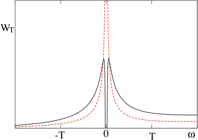
Figure 1: (Color online) A schematic sketch of the momentum integrated neutron scattering probability $W_{T}(\omega)$ at nonzero temperature. The probability for an isotropic magnet (O(3) $\sigma$-model) is shown by the black solid line. The probability for an easy-plane magnet (O(2) $\sigma$-model) is shown by the red dashed line.

The nontrivial point is that the quasielastic peak at $|\omega|\lesssim T$ differs from the previously known formula AA by the logarithmic term $-\tau d\omega/|\omega|\ln(T/|\omega|)/\ln(T/\Delta)$. The term is important to satisfy the spectral sum rule: the total quasielastic intensity at nonzero temperature must be equal to the elastic intensity at zero temperature

$$\int_{\sim-T}^{\sim T}W_{T}(\omega)d\omega\approx\int_{-\delta\rightarrow 0}^{+\delta\rightarrow 0}W_{0}(\omega)d\omega=V\ .$$ (15)

This sum rule must be valid with relative accuracy up to terms of the order of $\sim\tau\ll 1$. Without account of the logarithmic term the sum rule is violated. It is easy to see that the term reduces the total quasielastic intensity by two times. A simple heuristic derivation of the spectrum (9) is given in section IV, and a rigorous derivation based on the RG analysis is given in section V.

An easy-plane quantum magnet is described by the O(2) nonlinear $\sigma$-model. The long range magnetic order is also destroyed by a nonzero temperature, but in this case there is no a correlation length and no a “spin-wave gap”. Because of the Berezinsky-Kosterlitz-Thouless physics all correlators decay as powers of distance Chak . Our result for the nonzero temperature q-integrated neutron scattering probability in this case reads

$$O(2):$$ (16)

$$\frac{W_{T}(\omega)d\omega}{V}=\left\{\begin{array}[]{ll}\frac{1}{2}\tau T^{-\tau}\frac{d\omega}{|\omega|^{1-\tau}}&\ \ \ \ |\omega|\lesssim T\\ \sim 0&\ \ \ \ \omega\lesssim-T\\ \frac{d\omega}{4\pi\rho_{s}}&\ \ \ \ \omega\gtrsim T\end{array}\right.$$ (20)

The probability is sketched in Fig.1 by the red dashed line. The energy scale $\Delta$ plays a role in this case as well. Certainly it is not a gap any more, this is just the relevant energy scale. At $|\omega|\gg\Delta$ the intensity (16) is twice smaller than (9). This is because there is only one magnon in the O(2) case against two magnons in the O(3) case. On the other hand at $|\omega|\lesssim\Delta$ the O(2) intensity is much larger than the O(3) one. The spectral sum rule (15) is satisfied in this case as well because the elastic intensity is the same in both O(2) and O(3) cases. A heuristic derivation of the spectrum (16) is given in section IV, and a rigorous RG derivation is given in section V.

A uniform magnetic field, applied to an isotropic antiferromagnet, orients sublattice moments perpendicular to the field and therefore acts as a kind of easy plane anisotropy. This means that the magnetic field smoothly transfers the O(3) magnet to the O(2) magnet. If temperature is zero then the effect of the magnetic field acting on isotropic antiferromagnet is very simple and well understood. We consider here a nonzero temperature. For convenience we rescale the magnetic field, $g\mu_{B}B\rightarrow B$, where $g$ is the g-factor, and $\mu_{B}$ is Bohr magneton. If the magnetic field is larger than temperature, $B>T$, then obviously the quasielastic peak is described by the O(2) formula (16). If the magnetic field is very small, $B\ll\Delta$, then practically the quasielastic peak is described by the O(3) formula (9). The only nontrivial case is the case of the intermediate magnetic field, $\Delta\ll B\ll T$. Our result for the q-integrated spectrum in this case reads

$$O(3)\ \text{in\ magnetic\ field},\ \ \Delta\ll B\ll T:$$ (21)

$$\frac{W_{T}(\omega)d\omega}{V}=\left\{\begin{array}[]{ll}\frac{\tau}{2}\frac{B^{-\tau^{\ast}}d\omega}{|\omega|^{1-\tau^{\ast}}}\left[1-\tau\ln\left(\frac{T}{B}\right)\right]&\ \ \ |\omega|\lesssim B\\ \tau\frac{d\omega}{|\omega|}\left[1-\tau\ln\left(\frac{T}{|\omega|}\right)\right]&\ \ \ B\lesssim|\omega|<T\\ \sim 0&\ \ \ \omega\lesssim-T\\ \frac{d\omega}{2\pi\rho_{s}}&\ \ \ \omega\gtrsim T\end{array}\right.$$ (26)

where

$$\tau^{\ast}=\frac{\tau}{1-\tau\ln\left(T/B\right)}\ .$$ (27)

The probability (21) is sketched in Fig.2. Naturally, the spectrum (21) satisfies the spectral sum rule (15).

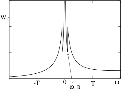
Figure 2: A schematic sketch of the momentum integrated neutron scattering probability $W_{T}(\omega)$ for isotropic antiferromagnet (O(3) $\sigma$-model) in the external magnetic field in the regime $\Delta\ll B\ll T$.

A heuristic derivation of the spectrum (21) is given in section IV, and a rigorous RG derivation is given in section V.

III Dependence of elastic/quasielastic neutron scattering intensity on magnetic field in a vicinity of a magnetic O(3) QCP

In this section we discuss enhancement of the staggered magnetization by applied external magnetic field. This effect was first pointed out for the square lattice Heisenberg antiferromagnet in Ref.zhitomirsky98, . In the present paper we stress that the effect is strongly enhanced in the vicinity of a magnetic QCP. To discuss this effect it is sufficient to consider the zero temperature case. At a finite temperature the integrated quasielastic intensity equals to the elastic intensity at zero temperature. The magnetic field changes the staggered magnetization,

$$\langle n_{z}\rangle \approx 1-\frac{1}{2}\langle n_{\perp}^{2}\rangle+\frac{1}{2}\langle n_{\perp}^{2}\rangle_{B=0}$$

$$= 1-\frac{1}{2V\chi_{\perp}}\sum_{\bm{k}}\left(\frac{1}{\omega_{\bm{k}}}-\frac{1}{\omega_{\bm{k},B=0}}\right)\ .$$

We remind that our normalization is $\langle n_{z}\rangle_{T=0,B=0}=1$. In the presence of external magnetic field the in-plane magnon remains gapless (easy plane), $\omega_{\bm{k}}=ck$, while the out-of-plane magnon becomes gapped com , $\omega_{\bm{k}}=\sqrt{c^{2}k^{2}+B^{2}}$. This results in the enhancement of the staggered magnetization,

$$\delta\langle n_{z}\rangle=\frac{1}{4\chi_{\perp}}\int\frac{d^{2}k}{(2\pi)^{2}}\left(\frac{1}{ck}-\frac{1}{\sqrt{c^{2}k^{2}+B^{2}}}\right)=\frac{|B|}{8\pi\rho_{s}}\ .$$ (29)

Clearly this formula is valid only if $\delta\langle n_{z}\rangle\ll 1$. There are two important points to note about Eq.(29): (i) the dependence on the magnetic field is linear, (ii) the dependence is enhanced approaching a QCP where the spin stiffness $\rho_{s}$ vanishes (The Eq. (29) is however inapplicable in the near vicinity of the QCP where the criterion $\delta\langle n_{z}\rangle\ll 1$ is violated), see e.g. Ref. Sachdev, .

To estimate magnitude of the effect (29) we refer to the simple model HSS , two coupled Heisenberg planes with spin 1/2, the position of the QCP is $g_{c}=J_{\perp}/J=2.525$. In the vicinity of the QCP the observed staggered magnetization $\mu$ and the spin stiffness scale as $\mu\propto(g_{c}-g)^{\beta}$, $\rho_{s}\propto(g_{c}-g)^{\nu}$ , where the critical indexes are related, $2\beta=(1+\eta)\nu$, see e.g. Refs. Chak, ; Chub, . The index $\eta\approx 0.03$ is very small, so practically $\nu\approx 2\beta$. The spin stiffness at $J_{\perp}=0$ is $\rho_{s0}\approx 0.2J$ and the staggered magnetic moment $\mu^{2D}\approx 0.6\mu_{B}$, see Ref. SZ, . Hence

$$\rho_{s}\sim 0.2J\left(\frac{\mu}{0.6\mu_{B}}\right)^{2}\ .$$ (30)

For further numerical estimates we refer to the experiment Haug09 performed with YBa₂Cu₃O_6.45. The experimental dependence of the quasielastic neutron scattering intensity on magnetic field is shown in Fig.3

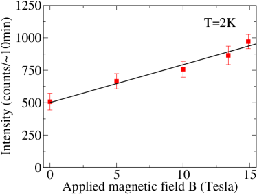
Figure 3: (Color online) YBa₂Cu₃O_6.45: The experimental dependence Haug09 of the elastic peak intensity on the external magnetic field at $T=2$ K. The intensity is measured at the incommensurate position of the neutron scattering peak. The line is the result of a linear fit to the data points.

Note that the compound is a superconductor with critical superconducting temperature $T_{c}=35K$. This is the second order superconductor, the magnetic field of several Tesla pretty much penetrates in the bulk, and therefore we disregard superconductivity in the analysis. The compound is very close to the magnetic QCP, the value of the static “staggered” moment is $\mu\sim 0.05\mu_{B}$, see Ref. Haug09, . Therefore, according to Eq.(30) the spin stiffness is about $\rho_{s}\sim 2\times 10^{-3}J$. With the magnetic field $B=15$ Tesla and with the characteristic cuprate exchange integral $J=1400K$, Eq. (29) gives the following field induced variation of the magnetization

$$\frac{\delta\mu}{\mu}=\frac{|B|}{8\pi\rho_{s}}\sim 0.3\ .$$ (31)

This value is very close to the data Haug09 presented in Fig.3 (Intensity is quadratic in magnetic moment, therefore $\delta I/{I}=2\delta\mu/{\mu}$). There is no doubt that the magnetic QCP observed in YBa₂Cu₃O_y is of a more complex nature than just a simple O(3) QCP, see a discussion in Ref. Milstein08, . Nevertheless, it is clear that generically Eq.(29) must be valid because it is based only on two physical inputs: gapless spin-wave spectrum and reduction of the effective spin stiffness in the vicinity of the QCP.

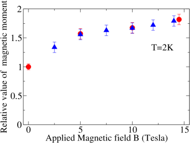
Figure 4: (Color online) La_1.9Sr_0.1CuO₄: The experimental dependence Lake02 of the static magnetic moment on the external magnetic field at $T=2$ K. The magnetic moment is measured at the incommensurate position of the neutron scattering peak. The data points shown by red circles are obtained from Fig.3a of Ref. Lake02, , and the data points shown by blue triangles are obtained from Fig.3b of Ref. Lake02, .

The La based compound La_2-xSr_xCuO₄ is very strongly disordered due to random positions of Sr ions. In addition the compound has a nonmonotonous dependence of the static magnetic moment on doping muofx (anomaly at $x\approx 0.12$). These two reasons complicate a comparison between theory and experiment. The magnetic field dependence of the static magnetic moment in La_1.9Sr_0.1CuO₄ has been measured by neutron diffraction. Lake02 The experimental magnetic moment versus magnetic field is plotted in Fig.4. The magnetic moment is normalized to its value at zero field. Fig.4 displays the quick growth from zero to 5 Tesla and then a slow linear dependence. A possible explanation of these data is based on the idea of magnetism induced around superconducting vortex core. DSZ An alternative explanation based on the approach developed in the present paper is that the steep dependence up to 5 Tesla is due to glassy effects related to random positions of Sr ions, and the slow dependence for $5<B<15$ is due to suppression of quantum fluctuations described by Eq.(29). Within this framework the effect observed in both YBa₂Cu₃O_6.45 and La_1.9Sr_0.1CuO₄ has the same physical origin.

IV Heuristic derivation of inelastic neutron scattering spectra at nonzero temperature

We start from derivation of Eq.(9) that describes quasielastic scattering from the isotropic antiferromagnet (the O(3) case). Let us consider the energy transfer $\omega$ much larger than the “spin wave gap” and somewhat smaller than temperature, $\Delta\ll\omega\lesssim T$. Hence the momentum transfer is $q\sim\omega/c$. The corresponding time/space scales, $\delta t\sim 1/\omega$, $\delta r\sim 1/q$, are much smaller than the time/space scales of slow thermal fluctuations that destroy the long-range AF order, $\delta t_{f}\sim 1/\Delta$, $\delta r_{f}\sim\xi$. Thus, the neutron makes a snapshot of the slowly fluctuating antiferromagnet, the AF order is untouched at the relevant scale. Hence, the formula (4) for the scattering probability is almost correct. One needs only to “erase” the elastic peak, and in the inelastic part to account for thermally excited magnons with the standard Bose occupation numbers

$$n_{\mathbf{k}}=\frac{1}{e^{\omega_{\mathbf{k}}/T}-1}\ .$$ (32)

Hence, (4) is transformed to

$$W(\omega,{\bm{q}})=2VA_{\bm{q}}^{2}\left[(n_{\mathbf{q}}+1)\delta(\omega-\omega_{\bm{q}})+n_{\mathbf{q}}\delta(\omega+\omega_{\bm{q}})\right]\$$ (33)

As usually the first term comes from the magnon emission and the second term comes from the magnon absorption. Integrating (33) over $q$ and expanding at $|\omega|\ll T$ one finds

$$W_{T}(\omega)d\omega\to\tau V\frac{d\omega}{|\omega|}\ .$$ (34)

To propagate the spectrum down to $\omega\sim\Delta$ we note that the power of $\omega$ is fixed by dimension. However, dimension does not forbid an additional logarithmic contribution, $W_{T}\to W_{T}\left[1+\mu\ln(T/|\omega|)\right]$, where $\mu\ll 1$ is some small coefficient. The logarithmic term must be negligible at $T\gtrsim|\omega|\gg\Delta$, where Eqs.(33),(34) have been derived, however it can be 100% important at $|\omega|\sim\Delta$. Imposing the spectral sum rule condition (15) one immediately finds that $\mu\approx-1/\ln(T/\Delta)\approx-\tau$. This concludes the heuristic derivation of the spectrum (9). Notice that the spectral sum rule uniquely determines the spectrum as soon as one takes the first power of logarithm. However, a priory, one cannot exclude higher powers, for example, $W_{T}\to W_{T}\left[1+\mu\ln(T/|\omega|)+\nu\ln^{2}(T/|\omega|)\right]$. Therefore, the presented simple heuristic derivation certainly cannot substitute a rigorous derivation. The rigorous derivation of (9) based on RG is given in Section V.

In the O(2) case (easy-plane magnet) the logic of derivation is very similar. In this case Eqs. (33) and (34) must be also valid in the regime $\Delta\ll\omega\lesssim T$. The only difference is that the prefactor in these Eqs. must be two times smaller because in the O(2) model there is only one magnon instead of two magnons in the O(3) model. However, propagation of these Eqs. to smaller $\omega$ is different because of the Berezinsky-Kosterlitz-Thouless physics in the O(2) case. In this case there is no a correlation length, all correlators decay as powers of appropriate variables Chak ; Chub . Therefore, the only possible correction to the spectrum (34) is an additional prefactor $(T/\omega)^{p}$, where $p\ll 1$. The quasielastic spectrum still has to satisfy the spectral sum rule (15). From here one immediately finds that $p=-\tau$ and this proves the validity of the spectrum (16). An RG derivation of the spectrum (16) is presented in the Section V.

Eq. (21) describes the quasielastic scattering from the isotropic antiferromagnet in the external magnetic field, $\Delta\ll B\ll T$. Obviously, at a frequency higher than the magnetic field, $B<|\omega|<T$, the field is not important and hence the spectrum (21) must coincide with (9). At $|\omega|<B$ the gapped magnon is switched off, the problem is effectively reduced to the O(2) case, and hence the shape of the spectrum must be the same as that in (16). However, one has to take care about thermal fluctuations with typical frequencies between $B$ and $T$. These fluctuations reduce value of the magnetization that comes to the effective O(2) $\sigma$-model regime,

$$\langle n_{z}\rangle^{2}=1\rightarrow\langle n_{z}\rangle^{2}=1-\langle n_{\perp}^{2}\rangle=1-\tau\ln\left(\frac{T}{B}\right)\ .$$ (35)

Neutron scattering is proportional to the magnetization squared, therefore, (35) presents another explanation of Eq.(9). Because of the reduction of number of active magnons, $2\rightarrow 1$, the intensity at $\omega=B-0$ must jump down by factor 2 compared to the intensity at $\omega=B+0$. Further evolution down in frequency is governed by the O(2) $\sigma$-model. However, we have defined the effective O(2) $\sigma$-model with $\langle n_{z}\rangle=1$ at the upper cutoff which is $B$ in this case instead of $T$ in (16). Therefore to apply (16) one has to renormalize magnetization back to unity, $\langle n_{z}\rangle\rightarrow 1$, and this implies that $\rho_{s}\rightarrow\rho_{s}^{\ast}=\rho_{s}\left[1-\tau\ln\left(\frac{T}{B}\right)\right]$. This explains why $\tau$ defined in (8) is replaced by $\tau^{\ast}$ given by (27). Notice that the spectrum (21) satisfies the spectral sum rule (15). Rigorous RG derivation of this spectrum is presented in the Section V.

V Renormalization Group (RG) analysis

To perform calculations of thermodynamic and dynamic properties we consider contribution of different momenta in small steps. To account for thermal fluctuations, we put ultraviolet cutoff $\Lambda$ on the theory (which is temperature $T/c\rightarrow T$ in the finite-temperature renormalized-classical regime) and follow the standard procedurePolyakov ; Nelson . Supposing that magnetic field acts along the $x$-axis and the order parameter is along the $z$-axis, we represent the vector $\mathbf{n}=(\pi_{x},\pi_{y},\sqrt{1-\pi^{2}})$ and introduce the two-component vector $\mathbf{\pi=}(\pi_{x},\pi_{y})$. In terms of the two-component field $\pi$ the Lagrangian becomes (now we use the imaginary time $t$, and set the spin-wave velocity equal to unity, $c=1$)

$$\mathcal{L} = \frac{\rho_{s}}{2}\int dtd^{2}x[(\partial\pi)^{2}+B^{2}\pi_{x}^{2}+h\pi^{2}$$ (36)

$$+(\mathbf{\pi}\partial\mathbf{\pi})^{2}+\frac{h}{4}\pi^{4}-4iB\pi^{2}\partial_{t}\pi_{c}-B^{2}$$

$$-\frac{1}{\rho_{s}}(\pi^{2}+\frac{1}{2}\pi^{4})]$$

where $\partial=(\nabla,\partial_{t}),$ and we have introduced the source field $h$ for the longitudinal ($n_{z}$) spin component. The terms in the first line of Eq. (36) correspond to the Lagrangian of the noninteracting spin waves, the other terms are responsible for the spin-wave interaction (the last term arises from the condition $n^{2}=1$).

Let consider the renormalization of parameters of the spin wave spectrum by the interaction. To first order in $1/\rho_{s}$ we have

$$\pi^{4} \rightarrow 2\pi^{2}\sum\nolimits_{i=x,y}\langle\pi_{i}^{2}\rangle+4\sum\nolimits_{i=x,y}\langle\pi_{i}^{2}\rangle\pi_{i}^{2}$$

$$-\langle\pi^{2}\rangle\langle\pi^{2}\rangle-2\sum\nolimits_{i=x,y}\langle\pi_{i}^{2}\rangle\langle\pi_{i}^{2}\rangle$$

$$(\pi_{i}\partial\pi_{i})^{2} \rightarrow \pi_{i}^{2}\langle(\partial\pi_{i})^{2}\rangle+(\partial\pi_{i})^{2}\langle\pi_{i}^{2}\rangle$$ (37)

$$-\langle\pi_{i}^{2}\rangle\langle(\partial\pi_{i})^{2}\rangle$$

After performing decouplings (V) we obtain up to a constant contribution

$$\mathcal{L} = \frac{{\rho_{s}}}{2}\int dtd^{2}x\left[\sum\nolimits_{i=x,y}(\partial\pi_{i})^{2}(1+\langle\pi_{i}^{2}\rangle)\right.$$

$$\left.+B^{2}\pi_{x}^{2}(1-\langle\pi_{x}^{2}\rangle)+h\pi^{2}+2B\pi^{2}\partial_{t}\pi_{y}+O(\pi^{4})\right]$$

where we have taken into account $\langle(\partial\pi_{i})^{2}\rangle-1/{\rho_{s}}=-m_{i}^{2}\langle\pi_{i}^{2}\rangle$; $m_{x}^{2}=B^{2}+h,$ $m_{y}^{2}=h$ are masses of $\pi_{x}$ and $\pi_{y}$ fields respectively. Rescaling the field $\pi\rightarrow(1+\langle\pi_{i}^{2}\rangle)^{-1/2}\pi$ to restore the coefficient at $(\partial\pi)^{2}$ we obtain

$$\mathcal{L} = \frac{{\rho_{s}}}{2}\int dtd^{2}x\left[(\partial\pi)^{2}+B^{2}\pi_{x}^{2}(1-2\langle\pi_{x}^{2}\rangle)\right.$$ (39)

$$+h\sum\nolimits_{i=x,y}\pi_{i}^{2}(1+\frac{1}{2}\langle\pi_{\overline{i}}^{2}\rangle-\frac{1}{2}\langle\pi_{i}^{2}\rangle)+$$

$$\left.+2B\pi^{2}\partial_{t}\pi_{y}+O(\pi^{4})\right]$$

where $\overline{x}=y$ and $\overline{y}=x.$ The corresponding renormalized parameters are

$$B_{R}^{2} = B^{2}(1-2\langle\pi_{x}^{2}\rangle)$$

$$h_{R}^{i} = h(1+\frac{1}{2}\langle\pi_{\overline{i}}^{2}\rangle-\frac{1}{2}\langle\pi_{i}^{2}\rangle)$$ (40)

From the performed rescaling we have in addition

$$\rho_{is}^{R}Z_{i}^{2}={\rho_{s}}(1+\langle\pi_{i}^{2}\rangle)$$ (41)

where $Z_{i}$ is the rescaling factor of the field $n_{i}$. Requiring similar to Polyakov ; Nelson $h^{R}\rho_{si}^{R}=Z_{i}(h\rho_{si}),$ we obtain

$$Z_{i}=1+\frac{1}{2}\langle\pi_{\overline{i}}^{2}\rangle+\frac{1}{2}\langle\pi_{i}^{2}\rangle$$ (42)

Therefore

$$Z_{x} = Z_{y}=1+\frac{1}{2}\langle\pi_{x}^{2}\rangle+\frac{1}{2}\langle\pi_{y}^{2}\rangle$$

$$\rho_{is}^{R} = {\rho_{s}}(1-\langle\pi_{\overline{i}}^{2}\rangle)$$ (43)

The renormalization factor for the $n_{z}$ field can be determined from the sublattice magnetization

$$\langle n_{z}\rangle=1-\frac{1}{2}\langle\pi_{x}^{2}\rangle-\frac{1}{2}\langle\pi_{y}^{2}\rangle$$ (44)

which implies $Z_{x}=Z_{y}=Z_{z}$. Similarly to the isotropic case Nelson , the obtained expressions for the renormalized parameters (43) can be used to formulate the renormalization group transformation. Below we consider the renormalized classical regime, $T\gg\max(\Delta,B)$.

As it is argued in Refs. Chak, ; Chub, , it is sufficient in the renormalized classical regime to account only for classical (zero Matsubara frequency) contributions to $\langle\pi_{i}^{2}\rangle$. Considering the contribution of infinitely thin layer in momentum space, we obtain ($\tau_{i}=T/(2\pi\rho_{s}^{i})$)

$$\frac{d\tau_{x}}{dl} = \tau_{x}\tau_{y},$$

$$\frac{d\tau_{y}}{dl} = \frac{\tau_{x}\tau_{y}}{1+e^{2l}B^{2}},$$

$$\frac{d\ln Z^{2}}{dl} = \frac{\tau_{x}}{1+e^{2l}B^{2}}+\tau_{y},$$ (45)

where $l=\ln(\Lambda/\mu)$ is the scaling parameter. The flow of the magnetic field can be neglected in the one-loop approximation.

For $B=0$ Eqs. (V) are equivalent to standard one-loop RG equations for 2D antiferromagnet Polyakov ; Nelson . Eqs. (V) are similar to those for the easy-plane case studied in Ref. IK1, , although differ from those due to presence of two spin stiffnesses instead of one. The other way of writing first two Eqs. (V) is

$$\frac{d\ln\tau_{x}}{dl} = \tau_{y},$$

$$\frac{d\ln\tau_{y}}{dl} = \frac{\tau_{x}}{1+e^{2l}B^{2}}\ .$$ (46)

Together with the last Eq. (V) this implies that $Z^{2}(l)/[\tau_{x}(l)\tau_{y}(l)]=1/\tau^{2}$ is the invariant of the flow.

At $e^{2l}B_{a}^{2}(l)\ll 1$ [$O(3)$ regime] we have $\tau_{x}(l)\approx\tau_{y}(l)$ such that

$$\frac{d\tau_{x,y}}{dl}=\tau_{x,y}^{2}$$ (47)

and $\tau_{x,y}(l)/Z(l)=\tau,$ which yields

$$\tau_{x}(l) \approx \tau_{y}(l)\approx\tau/(1-\tau l);$$

$$Z(l) \approx 1/(1-\tau l)$$ (48)

At $e^{2l}B_{a}^{2}(l)\sim 1$ the crossover from $O(3)$ to $O(2)$ regime occurs. At the crossover scale $l^{\ast}=\ln(\Lambda/B)$ we obtain $\tau^{\ast}\equiv\tau_{x}^{\ast}\approx\tau_{y}^{\ast}\approx\tau Z^{\ast}$ with

$$Z^{\ast}\approx 1/[1-\tau\ln(\Lambda/B)]$$ (49)

For $e^{2l}B_{a}^{2}(l)\gg 1$ [$O(2)$ regime] the flow of $\tau_{c}(l)$ is suppressed and we have $\tau_{y}(l)=\tau_{y}^{\infty}$=const,

$$\frac{d\ln Z^{2}}{dl}=\frac{d\ln\tau_{x}}{dl}=\frac{\tau_{y}^{\infty}}{2\pi}$$

where $\tau_{y}^{\infty}\simeq\tau^{\ast}$ up to logarithmic accuracy, such that

$$\tau_{x}(l) \approx \tau^{\ast}\exp[\tau^{\ast}(l-l^{\ast})]$$

$$Z^{2}(l) \approx Z^{\ast 2}\exp[\tau^{\ast}(l-l^{\ast})]$$ (50)

Representing $l=\ln(\Lambda/\mu)$ we obtain

$$\tau_{x}(\mu) \approx \tau Z^{\ast}(B/\mu)^{1/\ln(B/\Delta)}$$

$$Z^{2}(\mu) \approx Z^{\ast 2}(B/\mu)^{1/\ln(B/\Delta)}$$ (51)

where $Z^{\ast}$ is given by Eq. (49) and to one-loop order $\Delta=\Lambda\exp(-1/\tau)$ (Note that the two-loop corrections yield $\Delta$ given by Eq. (7), see Ref Chak, ). This power-law dependence corresponds to the Berezinsky-Kosterlitz-Thouless behavior of correlation functions (see below).

Now we discuss the behavior of correlation functions important for experimental data. From our scaling analysis we can obtain the transverse Green functions

$$\langle\langle n_{\mathbf{q}}^{i}|n_{-\mathbf{q}}^{i}\rangle\rangle_{i\omega} \equiv \int\nolimits_{0}^{1/T}dt\langle T[n_{\mathbf{q}}^{i}(t)n_{\mathbf{q}}^{i}(0)]\rangle e^{i\omega t}$$

$$= \langle\langle\pi_{\mathbf{q}}^{i}|\pi_{-\mathbf{q}}^{i}\rangle\rangle_{i\omega}=\frac{2\pi\tau_{i\mathbf{q}}}{TZ_{i\mathbf{q}}^{2}}\frac{1}{\omega^{2}+\omega_{i\mathbf{q}}^{2}}$$

where $\omega_{i\mathbf{q}}=\sqrt{\mathbf{q}^{2}+m_{i}^{2}}$, $m_{x}=B,$ $m_{y}=0,$ $\tau_{i\mathbf{q}},Z_{i\mathbf{q}}$ are obtained from the result of the solution of Eqs. (V) by substitution $l_{i}=\ln(T/\omega_{i\mathbf{q}})$. Therefore, we obtain the results for the functions at $|\mathbf{q}|\gg B$ in the renormalized classical regime

$$\langle\langle n_{\mathbf{q}}^{x}|n_{-\mathbf{q}}^{x}\rangle\rangle_{i\omega} = \langle\langle n_{\mathbf{q}}^{y}|n_{-\mathbf{q}}^{y}\rangle\rangle_{i\omega}=\frac{2\pi\tau_{x}}{TZ^{2}}\frac{1}{\mathbf{q}^{2}+\omega^{2}}$$ (53)

$$\simeq \frac{1}{\rho_{s}}\left(1-\tau\ln\frac{\Lambda}{|\mathbf{q|}}\right)\frac{1}{\mathbf{q}^{2}+\omega^{2}}$$

This result agrees with the result for the correlation function derived for the $O(3)$ model by Chakravarty, Halperin and NelsonChak . On the other hand, in the scaling limit $l\longrightarrow\infty$ we obtain from Eq. (V)

$$\frac{\tau_{y}(\mu)}{Z^{2}(\mu)}=\tau\left(1-\tau\ln\frac{\Lambda}{B}\right)\left(\frac{\mu}{B}\right)^{1/\ln(B/\Delta)}$$ (54)

which implies the results for the functions at $|\mathbf{q}|\ll B$

$$\langle\langle n_{\mathbf{q}}^{i}|n_{\mathbf{q}}^{i}\rangle\rangle_{\omega}=\frac{1}{\rho_{s}}\left(1-\tau\ln\frac{\Lambda}{B}\right)\left\{\begin{array}[]{cc}\frac{1}{B^{2}}&i=x\\ \frac{(|\mathbf{q}|/B)^{\alpha}}{q^{2}}&i=y\end{array}\right\}$$ (55)

with $\alpha=1/\ln(B/\Delta).$ In this regime we obtain the power law corrections to the Green functions, which are in agreement with the Berezinsky-Kosterlitz-Thouless solution of the O(2) model. Note, that both results, (53) and (55) fulfill the sumrule

$$\sum_{\mathbf{q},\omega}\left[\langle\langle n_{\mathbf{q}}^{x}|n_{\mathbf{q}}^{x}\rangle\rangle_{\omega}+\langle\langle n_{\mathbf{q}}^{y}|n_{\mathbf{q}}^{y}\rangle\rangle_{\omega}\right]=1$$ (56)

which is actually required for the total spectral weight including the longitudinal Green function. This shows that the contribution of the longitudinal Green function is contained implicitly in the calculated transverse Green functions, which seems to be the general property of the $1/S$ expansionNote .

For the structure factor, given by imaginary parts of the Green functions at the real axis, we obtain

$${W}(\mathbf{q},\omega) = \frac{n_{\omega}}{\pi}\sum\nolimits_{i=x,y}\mathrm{Im}\langle\langle n_{\mathbf{q}}^{i}|n_{-\mathbf{q}}^{i}\rangle\rangle_{\omega}$$

$$= \frac{\pi c^{2}n_{\omega}}{T\omega}\sum\nolimits_{i=x,y}\frac{\tau_{i\mathbf{q}}}{Z_{i\mathbf{q}}^{2}}\left[\delta(\omega-\omega_{i\mathbf{q}})+\delta(\omega+\omega_{i\mathbf{q}})\right]$$

where $n_{\omega}$ is the Bose function. Integration over $\mathbf{q}$ yields

$${W}(\omega)=\int\frac{d^{2}\mathbf{q}}{(2\pi)^{2}}{W}(\mathbf{q},\omega)$$ (58)

$$= \frac{{\pi}}{\omega^{2}}\int\frac{qdq}{2\pi}\sum_{i}\frac{\tau_{i\mathbf{q}}}{Z_{i\mathbf{q}}^{2}}\left[\delta(\omega-\omega_{iq})+\delta(\omega+\omega_{iq})\right]$$

$$= \frac{1}{2|\omega|}\sum_{i=x,y}\theta(\omega^{2}-m_{i}^{2})\frac{\tau_{i\omega}}{Z_{\omega}^{2}}$$

where $\tau_{i\omega}=\tau_{i}(l=\ln(T/|\omega|))$ and similar for $Z_{\omega}$.

In the O(3) regime $|\omega|>B$ where $\tau_{x\omega}/Z_{\omega}^{2}=\tau_{y\omega}/Z_{\omega}^{2}=\tau[1-\tau{\ln(\Lambda/|\omega|)}],$ we obtain

$${W}(\omega)=\frac{\tau}{|\omega|}\left(1-\tau\ln\frac{\Lambda}{|\omega|}\right)$$ (59)

which agrees with the result (9). In the O(2) regime ($|\omega|<B$)

$$\frac{\tau_{x\omega}}{Z_{\omega}^{2}} =$$ const

$$\frac{\tau_{y\omega}}{Z_{\omega}^{2}} = \tau\left(1-\tau\ln\frac{\Lambda}{B}\right)\left(\frac{|\omega|}{B}\right)^{\tau^{\ast}}$$ (60)

and

$${W}(\omega)=\frac{\tau}{2|\omega|}\left(1-\tau\ln\frac{\Lambda}{B}\right)\left(\frac{|\omega|}{B}\right)^{\tau^{\ast}}$$ (61)

in agreement with (21).

VI Conclusion

We have considered two dimensional quantum antiferromagnets. At zero temperature the antiferromagnets possess the long range order that results in the elastic Bragg peak observed in neutron scattering. At an arbitrary small but finite temperature the long range order is destroyed and hence the elastic Bragg peak is transformed to the quasielastic spectrum. We derive these spectra. The derived quasielastic spectrum for an isotropic antiferromagnet is given by Eq.(9) and the corresponding physics is determined by the finite correlation length. The derived spectrum (9) differs from the previously known answer AA by a logarithmic term that changes the integrated intensity by two times. The derived quasielastic spectrum for an easy plane antiferromagnet is given by Eq.(16) and the corresponding physics is determined by the Berezinsky-Kosterlitz-Thouless power law. An external uniform magnetic field drives a crossover from the isotropic antiferromagnet to the easy plane one. Hence the quasielastic spectrum evolves with the magnetic field. This evolution is described by Eq.(21).

An external uniform magnetic field, applied to an isotropic quantum antiferromagnet, suppresses quantum fluctuations. As a result the integrated intensity of elastic (quasielastic) neutron scattering grows linearly with applied external magnetic field, see Eq.(29). The dependence is significantly enhanced in the vicinity of the quantum critical point that separates magnetically ordered and magnetically disordered states, an estimate is given in Eq.(31). We believe that the observed enhancement of the quasielastic scattering in magnetic field in YBa₂Cu₃O_6.45, Ref. Haug09, , and in La_1.9Sr_0.1CuO₄, Ref. Lake02, , is due to this mechanism. Extension of the present analysis to include the magnetic incommensurability and contribution of conduction electrons is of a great interest.

VII Acknowledgements

We are grateful to J. Oitmaa and G. S. Uhrig who attracted our attention to the enhancement of staggered magnetization in magnetic field. We acknowledge discussions with A. I. Milstein. A. K. acknowledges Max-Planck Society for partial financial support within the Partnership Program. O.P.S acknowledges MPI-PKS, Dresden, where part of this work was performed within the framework of the Advanced Study Group ”Unconventional Magnetism in High Fields”.

References

- (1) A. Auerbach and D. P. Arovas, Phys. Rev. Lett., 61, 617 (1988).
- (2) A. Polyakov, Phys. Lett. B 59, 79 (1979).
- (3) Yu. A. Kosevich and A. Chubukov, JETP Letters, 43, 36 (1986); Sov. Phys. JETP 64, 654 (1986); M.I. Kaganov and A.V. Chubukov, Sov. Phys. Uspekhi 30, 1015 (1987).
- (4) S. Chakravarty, B. I. Halperin, and D. R. Nelson , Phys. Rev. B 39, 2344 (1989).
- (5) A. V. Chubukov, S. Sachdev, and J. Ye, Phys. Rev. B 49, 11919 (1994).
- (6) V. Hinkov, D. Haug, B. Fauque, P. Bourges, Y. Sidis, A. Ivanov, C. Bernhard, C. T. Lin, and B. Keimer, Science 319, 597 (2008).
- (7) D. Haug, V. Hinkov, A. Suchaneck, D. S. Inosov, N. B. Christensen, Ch. Niedermayer, P. Bourges, Y. Sidis, J. T. Park, A. Ivanov, C. T. Lin, J. Mesot, and B. Keimer, Phys. Rev. Lett. 103, 017001 (2009).
- (8) B. Lake, H. M. Ronnow, N. B. Christensen, G. Aeppli, K. Lefmann, D. F. McMorrow, P. Vorderwisch, P. Smeibidl, N. Mangkorntong, T. Sasagawa, M. Nohara, H. Takagi, T. E. Mason, Nature 415, 299 (2002).
- (9) Magnetic Properties of Layered Transition Metal Compounds, ed. L.J. de Jongh, Cluwer, Dordrecht, 1989.
- (10) A. I. Milstein and O. P. Sushkov, Phys. Rev. B 78, 014501 (2008).
- (11) Such a formulation is similar to the standard quantum electrodynamics one [see, e.g. Berestetskii V B, Lifshitz E M and Pitaevskii L P 1982 Quantum Electrodynamics (Course of Theoretical Physics Vol 4) 2nd ed. (Oxford: Reed)], where one starts with the fully renormalized (observed) charge and mass values. For Heisenberg model, this approach can be justified e.g. by the renormalization-group analysis or expansionChub .
- (12) M. E. Zhitomirsky and T. Nikuni, Phys. Rev. B 57, 5013 (1998).
- (13) Note that the formula is obvious without any calculations because projection of spin on magnetic field is conserved and for the out-of plane magnon .
- (14) S. Sachdev, Z. Phys. B 94, 469 (1994).
- (15) K. Hida, J. Phys. Soc. Jpn. 59, 2230 (1990); A. W. Sandvik and D. J. Scalapino, Phys. Rev. Lett. 72, 2777 (1994).
- (16) R. R. P. Singh, Phys. Rev. B 39, 9760 (1989); Zheng Weihong, J. Oitmaa, and C. J. Hamer, Phys. Rev B 43, 8321 (1991).
- (17) S. Wakimoto, R. J. Birgeneau, Y. S. Lee, G. Shirane, Phys. Rev. B 63, 172501 (2001).
- (18) E. Demler, S. Sachdev, and Y. Zhang, Phys. Rev. Lett. 87, 067202 (2001).
- (19) D. R. Nelson and R. A. Pelcovits, Phys. Rev. B 16, 2191 (1977).
- (20) V. Yu. Irkhin, A. Katanin, Phys. Rev. B 60, 2990 (1999).
- (21) By the same reason Schwinger boson approach (see, e.g., D. P. Arovas and A. Auerbach, Phys. Rev. B 38, 316 (1988)) overestimates the total spin Green function by a factor 3/2, since it counts the contribution of the longitudinal Green function, which is already contained in the transverse functions.