Detecting massive gravitons using pulsar timing arrays

Abstract

At the limit of weak static fields, general relativity becomes Newtonian gravity with a potential field that falls off as inverse distance, rather than a theory of Yukawa-type fields with finite range. General relativity also predicts that the speed of disturbances of its waves is $c$, the vacuum light speed, and is non-dispersive.

For these reasons, the graviton, the boson for general relativity, can be considered to be massless. Massive gravitons, however, are features of some alternatives to general relativity. This has motivated experiments and observations that, so far, have been consistent with the zero mass graviton of general relativity, but further tests will be valuable.

A basis for new tests may be the high sensitivity gravitational wave experiments that are now being performed, and the higher sensitivity experiments that are being planned. In these experiments it should be feasible to detect low levels of dispersion due to nonzero graviton mass. One of the most promising techniques for such a detection may be the pulsar timing program that is sensitive to nano-Hertz gravitational waves.

Here we present some details of such a detection scheme. The pulsar timing response to a gravitational wave background with the massive graviton is calculated, and the algorithm to detect the massive graviton is presented. We conclude that, with $90\%$ probability, massles gravitons can be distinguished from gravitons heavier than $3\times 10^{-22}$ eV (Compton wave length $\lambda_{\rm g}=4.1\times 10^{12}$ km), if biweekly observation of 60 pulsars are performed for 5 years with pulsar RMS timing accuracy of 100 ns. If 60 pulsars are observed for 10 years with the same accuracy, the detectible graviton mass is reduced to $5\times 10^{-23}$ eV ($\lambda_{\rm g}=2.5\times 10^{13}$ km); for 5-year observations of 100 or 300 pulsars, the sensitivity is respectively $2.5\times 10^{-22}$ ($\lambda_{\rm g}=5.0\times 10^{12}$ km) and $10^{-22}$ eV ($\lambda_{\rm g}=1.2\times 10^{13}$ km). Finally, a 10-year observation of 300 pulsars with 100 ns timing accuracy would probe graviton masses down to $3\times 10^{-23}$ eV ($\lambda_{\rm g}=4.1\times 10^{13}$ km).

1. Introduction

Although a complete quantum version of gravitation has not yet been achieved (Smolin, 2003; Kiefer, 2006), in the weak field, linearized limit quantization of gravitation can be carried out. One can therefore ask phenomenologically whether or not the graviton in a gravity theory is massive (Rubakov & Tinyakov, 2008; Goldhaber & Nieto, 2010). Up to now the most successful theory of gravitation is general relativity (Will, 1993; Stairs, 2003; Will, 2006; Damour, 2007; Kramer & Wex, 2009). The quantization of its weak field limit (see Gupta (1952) and references therein) shows that its gravitational interaction is mediated by spin-2 massless bosons, the so called gravitons. Recently, attention has turned to this question due to both observational and theoretical advances.

On the theoretical side there is the issue of the vDVZ discontinuity (Iwasaki, 1970; van Dam & Veltman, 1970; Zakharov, 1970), the prediction that for a massive graviton, light deflection is greater than in general relativity by the factor 4/3, no matter how small the mass. If this were true, despite its paradoxical nature, then classical tests of starlight deflection would rule out massive gravitons. But recently, resolutions have been proposed to the vDVZ paradox, so that massive gravitons cannot be ruled out (Vainshtein, 1972; Visser, 1998; Deffayet et al., 2002; Damour et al., 2003; Finn & Sutton, 2002).

On the theoretical side also, advances in higher-dimensional theories have led to graviton mass-like features (e.g., DGP model by Dvali et al. (2000)); meanwhile, because of possible issues with standard gravitation from solar system scale (Anderson et al., 1998, 2008) to cosmological scale (Sanders & McGaugh, 2002), interest has been growing in alternative gravity theories, some of which predict massive gravitons (Dvali et al., 2000; Alves et al., 2009; Eckhardt et al., 2010). There is, therefore, considerable motivation for experimental or observational tests of whether the graviton can be massive.

The literature contains many estimates for an upper limit on the graviton mass, estimates that differ by many orders of magnitude. An early limit of $8\times 10^{4}$ eV (Hare, 1973) was based on considerations of a graviton decay to two photons. At about the same time Goldhaber & Nieto (1974) used the assumption that clusters of galaxies are bound by more-or-less standard gravity to infer an upper limit of $2\times 10^{-29}h_{0}$ eV, where $h_{0}$ is the Hubble constant in units of 100 km s^-1 Mpc^-1. By using the effect of graviton mass on the generation of gravitational waves by a binary, and the rate of binary inspiral inferred from the timing of binary pulsars, Finn & Sutton (2002) inferred an upper limit of $7.6\times 10^{-20}$ eV. Choudhury et al. (2004) considered the effect of a graviton mass on the power spectrum of weak lensing; with assumptions about dark energy and other paramters, they estimated a upper limit of $7\times 10^{-32}$ eV for the graviton mass. Reviews about these techniques can be found, e.g. , in Goldhaber & Nieto (2010); Particle Data Group (2008); Will (2006).

These upper limits are all of value, since they are based on different assumptions about the phenomenological effects of graviton mass. Most of the estimates are based on the effects of graviton mass on the static field of a source, typically assuming a Yukawa potential, though this may not be the general case for a particular theory of gravity, such as fifth force theories, or MOND-type theories (Will, 1998; Maggiore, 2008). In view of the lack of a theory of the graviton, it is important to have upper limits based on different phenomenological implications of graviton mass.

The mass limit of Finn & Sutton (2002) is based on the effect of graviton mass on the generation of gravitational waves, not on their propagation, but the dispersion relation for propagation is also an important independent approach to a mass limit, as has been recently suggested by a number of groups (Will, 1998; Larson & Hiscock, 2000; Cutler et al., 2003; Stavridis & Will, 2009). Questions about this method are timely since the detection of gravitational waves is expected in the near future, thanks to the progress with present ground-based laser interferometers, possible future space-based interferometers (Hough & Rowan, 2000; Hough et al., 2005), and pulsar timing array projects (Sallmen et al., 1993; Stappers et al., 2006; Manchester, 2006; Hobbs et al., 2009b).

The pulsar timing array is a unique technique to detect nano-Hertz gravitational waves by timing millisecond pulsars, which are very stable celestial clocks. It turns out that a stochastic gravitational wave background leaves an angular dependent correlation in pulsar timing residuals for widely spaced pulsars (Hellings & Downs, 1983; Lee et al., 2008). That is, the correlation $C(\theta)$ between timing residual of pulsar pairs is a function of angular separation $\theta$ between the pulsars. One can analyse the timing residual and test such a correlation between pulsar timing residuals to detect gravitational waves (Jenet et al., 2005). We find in this paper that if the graviton mass is not zero, the form of $C(\theta)$ is very different from that given by general relativity. Thus by measuring this graviton mass dependent correlation function, we can also detect the massive graviton.

The outline of this paper is as follows. The mass of the graviton is related to the dispersion of gravitational waves in § 2. The pulsar timing responses to a plane gravitational wave and to a stochastic gravitational wave background in the case of a massive graviton are calculated in § 3. The massive graviton induces effects on the shape of pulsar timing correlation function, which is derived in § 4, while the detectability of a massive gravitational wave background is studied in § 5. The algorithm for detect massive graviton using a pulsar timing array, and the sensitivity of that algorithm are examined in § 6. We discuss several related issues, and conclude in § 7.

2. Gravitational Waves with Massive Gravitons

We incorporate the massive graviton into the linearized weak field theory of general relativity (Gupta, 1952; Arnowitt & Deser, 1959; Weinberg, 1972). For linearized gravitational waves, specifying the graviton mass is equivalent to specifying the gravitational wave (GW) dispersion relation that follows from the special relativistic relationship

$$E^{2}=p^{2}c^{2}+m^{2}c^{4},$$ (1)

where $c$ is the light velocity, $E$ is energy of the particle, and $p$ and $m$ are the particle’s momentum and rest mass respectively. One can derive the corresponding dispersion relation from Eq. (1) by replacing the momentum by ${\bf p}=\hbar{\bf k}_{g}$ and the energy by $E=\hbar\omega_{g}$, where $\hbar$ is the reduced Planck constant, with ${\bf k}_{g}$ and $\omega_{g}$ respectively the GW wave vector and the angular frequency. With these replacements, the dispersion relation for a massive vacuum GW graviton propagating in the $z$ direction reads

$${\bf{k_{\rm g}}}({\omega_{\rm g}})=\frac{\left({\omega_{\rm g}}^{2}-{\omega_{\rm cut}}^{2}\right)^{\frac{1}{2}}}{c}\,{\hat{\rm\bf e}_{z}\,\!}\,,$$ (2)

where ${\hat{\rm\bf e}_{z}\,\!}$ is the unit vector in the $z$ direction. If the gravitational wave frequency ${\omega_{\rm g}}$ is less than the cut-off frequency $\omega_{\rm cut}\equiv{m_{\rm g}}c^{2}/\hbar$, then the wave vector becomes imaginary, indicating that the wave attenuates, and does not propagate. (The equivalent phenomena for electromagnetic waves can be found in §87 of Landau & Lifshitz (1960)).

At a space-time point $(t,{\bf r})$, the spatial metric perturbation due to a monochromatic GW is

$$h_{ab}(t,{\bf r})=\Re\left[\sum_{P=+,\times}A^{P}{\epsilon}^{P}_{ab}e^{i[{\omega_{\rm g}}t-{\bf r}\cdot{\bf{k_{\rm g}}}({\omega_{\rm g}})]}\right],$$ (3)

where $\Re$ indicates the real part, and where the $a,b$ range over spacetime indicts from 0 to 3. The summation is performed over the polarizations of the GW. Since we are not assuming that general relativity is the theory of gravitation, we could, in principle, have as many as six polarization states. For definiteness, however, and to most clearly show how pulsar timing probes graviton mass, we will confine ourselves in this paper to only the two standard polarization modes of general relativity, denoted $+$ and $\times$, the usual ‘TT” gauge (see Appendix A A for the details). Thus, the polarization index takes on only the values $P=+,\times$, with $A^{P}$ and ${\epsilon}^{P}$ standing for the amplitude and polarization tensors for the two transverse traceless modes.

The polarization tensor ${\epsilon}^{P}$ is described in terms of an orthonormal 3-dimensional frame associated with the GW propagating direction. Let the unit vector in the direction of GW propagation be ${\hat{\rm\bf e}_{z}\,\!}$; we can choose the other two mutually orthogonal unit vectors ${\hat{\rm\bf e}_{x}\,\!},{\hat{\rm\bf e}_{y}\,\!}$ to be both perpendicular to ${\hat{\rm\bf e}_{z}\,\!}$. In terms of these three vector, ${\hat{\rm\bf e}_{z}\,\!},{\hat{\rm\bf e}_{x}\,\!}$ and ${\hat{\rm\bf e}_{y}\,\!}$, the polarization tensors are given as

$${\epsilon}^{+}_{ab}={\hat{\rm\bf e}_{x}\,\!}_{a}{\hat{\rm\bf e}_{x}\,\!}_{b}-{\hat{\rm\bf e}_{y}\,\!}_{a}{\hat{\rm\bf e}_{y}\,\!}_{b},$$

$${\epsilon}^{+}_{ab}={\hat{\rm\bf e}_{x}\,\!}_{a}{\hat{\rm\bf e}_{y}\,\!}_{b}+{\hat{\rm\bf e}_{y}\,\!}_{a}{\hat{\rm\bf e}_{x}\,\!}_{b}\,.$$ (4)

Since the polarization tensors are purely spatial, we will have only spatial components of the metric perturbations. For a stochastic gravitational wave background, these metric perturbations are a superposition of monochromatic GWs with random phase and amplitude, and can be written as

$$h_{ij}(t,r^{i})=\sum_{P=+,\times}\int_{-\infty}^{\infty}df_{\rm g}\int d\Omega\,h^{P}(f_{\rm g},{\hat{\rm\bf e}_{z}\,\!})\,{\epsilon}^{P}_{ij}({\hat{\rm\bf e}_{z}\,\!})e^{i[{\omega_{\rm g}}t-{\bf k}_{g}({\omega_{\rm g}})\cdot{\bf r}}],$$ (5)

where $f_{\rm g}={{\omega_{\rm g}}}/{2\pi}$ is the GW frequency, $\Omega$ is solid angle, spatial indices $i,j$ run from 1 to 3, and $h^{P}$ is the amplitude of the gravitational wave propagating in the direction of ${\hat{\rm\bf e}_{z}\,\!}$ per unit solid angle, per unit frequency interval, in polarization state $P$. If the gravitational wave background is isotropic, stationary and independently polarized, we can define the characteristic strain $h_{c}^{P}$ according to (Maggiore, 2000; Lee et al., 2008), and can write

$$\langle h^{P}(f_{\rm g},{\hat{\rm\bf e}_{z}\,\!})h^{\star P^{\prime}}(f_{\rm g}^{\prime},{\hat{\rm\bf e}_{z}\,\!}^{\prime})\rangle=\frac{|h_{c}^{P}|^{2}}{16\pi f_{\rm g}}\delta_{PP^{\prime}}\delta(f_{\rm g}-f_{\rm g}^{\prime})\delta({\hat{\rm\bf e}_{z}\,\!}-{\hat{\rm\bf e}_{z}\,\!}^{\prime}),$$ (6)

where the $\star$ stands for the complex conjugate and $\langle\rangle$ is the statistical ensemble average. The symbol $\delta_{PP^{\prime}}$ is the Kronecker delta for polarization states; $\delta_{PP^{\prime}}=0$ when $P$ and $P^{\prime}$ are different, and $\delta_{PP^{\prime}}=1$, when $P$ and $P^{\prime}$ are the same. With the relationships above one can show that

$$\langle h_{ab}(t)h_{ab}(t)\rangle=\sum_{P=+,\times}\int_{0}^{\infty}\frac{|h_{c}^{P}|^{2}}{f_{\rm g}}df_{\rm g}\,.$$ (7)

3. Single Pulsar Timing Residuals Induced by a Massive Gravitational Wave Background

We now turn to the calculation of the pulsar timing effects due to the stochastic gravitational wave background prescribed by Eq. (5). That background is composed of monochromatic plane wave with random phase and with amplitude determined from some chosen spectrum. We can then first calculate the pulsar timing effect due to a monochromatic plane wave, and then add together all contributions to find the effects of a stochastic background.

In the weak field case, the time component of the null geodesic equations for photons is (Liang, 2000; Hobbs et al., 2009a)

$$\frac{d\omega}{d\lambda}+\frac{\omega^{2}}{2}\frac{\partial{h_{ij}}}{\partial t}\hat{\rm\bf n}^{i}\hat{\rm\bf n}^{j}=0\,.$$ (8)

Here $\omega$ is the angular frequency for the photon, $\hat{\rm\bf n}^{i}$ is the direction from the observer (Earth) to the photon source (pulsar), and $\lambda$ is an affine parameter along the photon trajectory, normalized so that in the Minkowski background $dt/d\lambda=\omega$. From this geodesic equation, the frequency shift of a pulsar timing signal induced by a monochromatic, plane, massive graviton GW is

$$\frac{\Delta\omega(t)}{\omega}=-\,\frac{\hat{\rm\bf n}^{i}\hat{\rm\bf n}^{j}}{2\left(1+({c}/{{\omega_{\rm g}}}){\rm\bf{k_{\rm g}}}\cdot\hat{\rm\bf n}\right)}\left[h_{ij}(t,0)-h_{ij}(t-|{\rm\bf D}|/c,{\rm\bf D})\right],$$ (9)

where it is assumed that the observer is at the coordinate origin and that $\rm\bf D$ is the displacement vector, in the background, from the observer to the pulsar. Equation (9) is a minor generalization of the relationship for zero-mass gravitons given in many references (Estabrook & Wahlquist (1975); Sazhin (1978); Detweiler (1979); Lee et al. (2008)). It is clear that the frequency shift of the pulsar timing signal only involves the metric perturbations at the observer, i.e., the term $h_{ij}(t,0)$, and the metric perturbation at the pulsar, i.e., the term $h_{ij}(t,\rm\bf D)$. The dispersion relation of the GWs enters, through the denominator, in the geometric factor $(1+c{\rm\bf{k_{\rm g}}}\cdot\hat{\rm\bf n}/{\omega_{\rm g}})$ and well as the phase difference between the GW at the earth $h_{ij}(t,0)$ and the GW at the pulsar $h_{ij}(t-|{\rm\bf D}|/c,{\rm\bf D})$. The induced pulsar timing residuals R(t) are given by the temporal integration of the above frequency shift at Earth, thus

$$R(t)=\int_{0}^{t}\frac{\Delta\omega(\tau)}{\omega}d\tau.$$ (10)

The equations Eq. (5), (9), and (10) determine the response of pulsar timing to a monochromatic plane GW. One can show the pulsar timing residual $R(t)$ induced by the stochastic GW background is

$$R(t)=\frac{i}{2}\sum_{P=+,\times}\int_{-\infty}^{\infty}df_{\rm g}\int d\Omega\frac{\hat{\rm\bf n}^{i}\hat{\rm\bf n}^{j}}{\left({\omega_{\rm g}}+c{\rm\bf{k_{\rm g}}}\cdot\hat{\rm\bf n}\right)}h^{P}(f_{\rm g},{\hat{\rm\bf e}_{z}\,\!}){\epsilon}^{P}_{ij}({\hat{\rm\bf e}_{z}\,\!})\left[1-e^{-i{\rm\bf{k_{\rm g}}({\omega_{\rm g}})\cdot D}}\right]\left[1-e^{i{\omega_{\rm g}}t}\right].$$ (11)

This is, for example, a minor modification of Eq. (A9) given by Lee et al. (2008). As we pointed out shortly before, the massive graviton dispersion relation enters via the term ${\omega_{\rm g}}+c{\rm\bf{k_{\rm g}}}\cdot\hat{\rm\bf n}$ as in Eq.( 9) and the term $1-e^{-i{\rm\bf{k_{\rm g}}({\omega_{\rm g}})\cdot D}}$, which comes from the phase difference between pulsar term and earth term.

After the nonobservable zero frequency component is removed, the auto-correlation function $\langle R(t)R(t+\tau)\rangle$ can be calculated by replacing the statistical ensemble average with the time average,

$$\langle R(t)R(t+\tau)\rangle=\sum_{P=+,\times}\int_{-\infty}^{\infty}df_{\rm g}\int d\Omega\,\frac{|h_{c}^{P}|^{2}}{32\pi f_{\rm g}}\left[\frac{{\epsilon}^{P}_{ij}\hat{\rm\bf n}^{i}\hat{\rm\bf n}^{j}}{{\omega_{\rm g}}+c{\rm\bf{k_{\rm g}}\cdot\hat{\rm\bf n}}}\right]^{2}\left[1-\cos\left(\frac{D}{c}({\omega_{\rm g}}+c{\rm\bf{k_{\rm g}}\cdot\hat{\rm\bf n}})\right)\right]e^{i{\omega_{\rm g}}\tau}\,,$$ (12)

where $D=|{\rm\bf D}|$ is the pulsar distance. The folded timing residual power spectra $S_{\rm R}(f_{\rm g})$ is defined to be the Fourier transform of the autocorrelation function of the timing residual,

$$S_{\rm R}(f_{\rm g})=2\int_{-\infty}^{\infty}\langle R(t)R(t+\tau)\rangle e^{-2\pi if_{\rm g}\tau}d\tau,$$ (13)

for which the explicit result is

$$S_{\rm R}(f_{\rm g})=\sum_{P=+,\times}\int d\Omega\,\frac{|h_{c}^{P}|^{2}}{16\pi f_{\rm g}}\left[\frac{{\epsilon}^{P}_{ij}\hat{\rm\bf n}^{i}\hat{\rm\bf n}^{j}}{{\omega_{\rm g}}+c{\rm\bf{k_{\rm g}}\cdot\hat{\rm\bf n}}}\right]^{2}\left[1-\cos\left(\frac{D}{c}({\omega_{\rm g}}+c{\rm\bf{k_{\rm g}}\cdot\hat{\rm\bf n}})\right)\right].$$ (14)

For a power-law stochastic GW background, the power spectra of the induced pulsar timing residual is (see Appendix for the details)

$$S_{\rm R}(f_{\rm g})=\sum_{P=+,\times}\frac{|h_{c}^{P}(f_{\rm g})|^{2}}{24\pi^{2}f_{\rm g}^{3}}\eta(f_{\rm g}),$$ (15)

where the $\eta(f_{\rm g})$ is

$$\eta(f_{\rm g})=\left\{\begin{array}[]{c c}\frac{-4\zeta^{3}+6\zeta+3\left(\zeta^{2}-1\right)\log\left(\frac{\zeta+1}{1-\zeta}\right)}{2\zeta^{5}}&\textrm{if $f_{\rm g}>f_{\rm cut}$}\\ 0&\textrm{if $f_{\rm g}\leq f_{\rm cut}$}\end{array}\right.$$

and

$$\zeta=\sqrt{1-\frac{\omega_{\rm cut}^{2}}{{\omega_{\rm g}}^{2}}}\quad\quad\quad\omega_{\rm cut}\equiv{m_{\rm g}}c^{2}/\hbar\,.$$ (16)

One can see that $\eta(f_{\rm g})$ is the spectral correction factor for massive GW backgrounds, if compared with the case of general relativistic GW background (Lee et al., 2008), where $\eta$ is equal to unity. To show the frequency dependence of the graviton mass effect, $\eta(f_{\rm g})$ is plotted in Fig. 1.

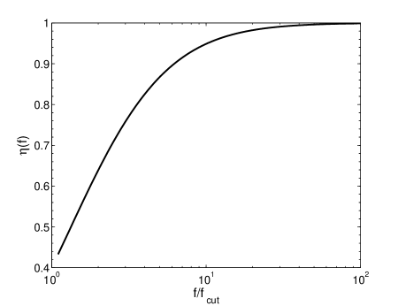
Figure 1.— The value of $\eta(f)$ as a function of GW frequency $f$ in units of the cut-off frequency $f_{\rm cut}$. When the GW frequency becomes much larger than the cut-off frequency, $\eta$ approaches unity, which means that the timing residuals approach those of the massless GW case. At the other extreme, for $f_{\rm g}$ close to $f_{\rm cut}$, the power in the timing residuals is minimal.

When $f_{\rm g}>f_{\rm cut}$, a convenient polynomial approximation of $\eta(f)$ with maximal error of $1.5\%$ is

$$\eta(f_{\rm g})=-0.7764\left(\frac{f_{\rm cut}}{f_{\rm g}}\right)^{4}+1.748\left(\frac{f_{\rm cut}}{f_{\rm g}}\right)^{3}-1.001\left(\frac{f_{\rm cut}}{f_{\rm g}}\right)^{2}-0.5868\,\frac{f_{\rm cut}}{f_{\rm g}}+1.012\,.$$ (17)

A least-squares polynomial fitting technique was used to calculate the coefficients in the above equation. The RMS level $\sigma_{\rm R}$ of the timing residual power is defined to be $\sigma_{\rm R}^{2}=\int_{0}^{\infty}S_{\rm R}(f)df$. The spectra of GW backgrounds generated by various astrophysical processes are usually summarized as power-law spectra with power index $\alpha$, i.e. the characteristic strain of GWs is $h_{\rm c}=A_{\rm c}(f/f_{0})^{\alpha}$. For such power-law spectra, the RMS level of corresponding pulsar timing residuals is

$$\sigma_{\rm R}^{2}\simeq\frac{A_{\rm c}^{2}f_{\rm L}^{2\alpha}}{f_{0}^{2\alpha}}\left(\beta_{1}\frac{f_{\rm cut}^{4}}{f_{\rm L}^{6}}+\beta_{2}\frac{f_{\rm cut}^{3}}{f_{\rm L}^{5}}+\beta_{3}\frac{f_{\rm cut}^{2}}{f_{\rm L}^{4}}+\beta_{4}\frac{f_{\rm cut}}{f_{\rm L}^{3}}+\beta_{5}\frac{1}{f_{\rm L}^{2}}\right),$$ (18)

where the constants $\beta_{1}\dots\beta_{5}$ take following values

$$\beta_{1} = 3.278\times 10^{-3}(\alpha-3)^{-1},$$

$$\beta_{2} = 1.476\times 10^{-2}(5-2\alpha)^{-1},$$

$$\beta_{3} = 4.226\times 10^{-3}(\alpha-2)^{-1},$$

$$\beta_{4} = 4.955\times 10^{-3}(2\alpha-3)^{-1},$$

$$\beta_{5} = 4.272\times 10^{-3}(1-\alpha)^{-1},$$ (19)

and the $f_{\rm L}={\rm Max}[T^{-1},f_{\rm cut}]$ is the larger of the following two frequencies: (1) the frequency cut-off ($T^{-1}$) due to the finite length time span $T$ of observation; (2)  the intrinsic frequency cut-off $f_{\rm cut}={\omega_{\rm cut}}/(2\pi)$ due to graviton mass.

One can derive an upper limit for the GW velocity using single pulsar timing data, because of the surfing effect (Baskaran et al., 2008b); but it is unlikely that one can use single pulsar timing data to constrain the graviton mass (Baskaran et al., 2008a). Because of the correction factor $\eta(f_{\rm g})$ (see Fig. 1), the graviton mass reduces the GW induced pulsar timing residuals. This prevents us from constraining the graviton mass using the amplitude of single pulsar timing residuals. However, as explained in the next section, the cross correlation between pulsar timing residuals from different directions will help us in detecting the graviton mass.

4. The Angular Dependent Correlation Between Pulsars

A stochastic GW background leaves a correlation between timing residuals of pulsars pairs (Hellings & Downs, 1983; Lee et al., 2008). Such a correlation, $C(\theta)$, depends on the angular distance $\theta$ between two pulsars. It turns out that the graviton mass changes the shape of this correlation function. One can therefore detect a massive graviton by examining the shapes of pulsar timing correlation functions.

As shown in Appendix B, the pulsar timing cross-correlation function for a massive GW background depends on the graviton mass, specific power spectra of GW background, and observation schedule. In this way, an analytical expression for the cross-correlation function would not be possible. We use Monte-Carlo simulations in this paper to determine the shape of the correlation function for GW backgrounds with a power-law spectra. In the Monte-Carlo simulations for $C(\theta)$, we randomly choose pulsars from an isotropic distribution over sky positions. We then hold constant these pulsar positions and calculate the angular separation $\theta$ between every pair of pulsars. Next, to simulate the power-law GW background, we generate $10^{4}$ monochromatic waves, choosing random phase, and choosing the amplitude from the power-law $h_{\rm c}=A_{\rm c}(f/f_{0})^{\alpha}$, where we take $\alpha=-2/3$ (Phinney, 2001; Jaffe & Backer, 2003; Wyithe & Loeb, 2003; Enoki et al., 2004; Sesana et al., 2004; Wen et al., 2009). The timing residuals are calculated using Eq. (9) and (10). Then, the cross-correlation function, $C(\theta)$, between pulsar pairs is calculated. We repeat such processes and average over the angular dependent correlation function $C(\theta)$ until the change in $C(\theta)$ is less than $0.1\%$. The averaged correlation function is then smoothed by fitting an eighth order Legendre polynomial (see Lee et al. (2008) for the details). This smoothed $C(\theta)$ is the correlation function we need. The $C(\theta)$ are plotted for various parameters in Fig. 2. We also check the results by choosing different sets of pulsars to make sure the $C(\theta)$ is not sensitive to the details of the random pulsar samples. As the $C(\theta)$ is the statistical expectation of the correlation function, we call it the theoretical correlation function in contrast with the observed correlation function defined in the next section.

As one may expect, the massive graviton has stronger effects for data from long observing periods than from short periods. One can see this by comparing the 5-year and 10-year correlation functions given in Fig. 2, where curves corresponding to the same range of graviton mass show considerably greater deviations from the massless case in the 10-year correlation function than in the 5-year one.

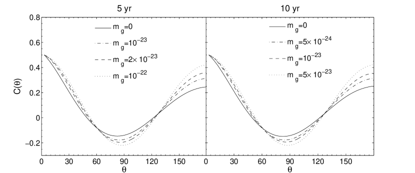
Figure 2.— The atlas for cross-correlation functions $C(\theta)$. The label of each curve indicates the corresponding graviton mass in units of electron-volts (eV). The left panel shows the correlation functions for a 5 year bi-weekly observation. The right panel shows correlation functions for 10-years of bi-weekly observations. We take $\alpha=-2/3$ for these results. These correlation are normalized such that the $C(0)=0.5$ for two different pulsars.

5. An Estimate of the Detectability of a Gravitational Wave Background with a Massive Graviton

As we have explained, the massive graviton reduces the pulsar timing response to GWs through the correction factor $\eta(f_{\rm g})$. In this way, a non-zero graviton mass reduces the pulsar timing array sensitivity for detecting a GW background. It is interesting to know how the sensitivity changes, if the graviton is massive.

The stochastic GW background is detected by comparing the measured cross-correlation function $c(\theta_{l})$ with the theoretical correlation $C(\theta)$ calculated in previous section. Here, the measured cross-correlation function $c(\theta_{l})$ is defined by

$$c(\theta_{m})=\frac{\sum_{l=0}^{N-1}(R_{a}(t_{l})-\overline{R_{a}(t_{l})}\;)(R_{b}(t_{l})-\overline{R_{b}(t_{l})}\;)}{\sqrt{\sum_{l=0}^{N-1}(R_{a}(t_{l})-\overline{R_{a}(t_{l})}\;)^{2}\sum_{l=0}^{N-1}(R_{b}(t_{l})-\overline{R_{b}(t_{l})}\;)^{2}}}\ ,$$ (20)

where the $R_{a}(t_{l})$ and $R_{b}(t_{l})$ are the timing residuals of pulsar ‘a’ and ‘b’ at time $t_{l}$ and $N$ is the number of observations. The $\overline{R_{b}(t_{l})}=\sum_{l=0}^{N-1}R_{b}(t_{l})/N$ and $\overline{R_{a}(t_{l})}=\sum_{l=0}^{N-1}R_{a}(t_{l})/N$. The $\theta_{m}$ is the angle between the direction pointing to pulsar ‘a’ and the direction pointing to pulsar ‘b’. Given $N_{\rm p}$ pulsars, the index $m$ runs from 1 to the number of pulsar pairs $M=(N_{\rm p}-1)N_{\rm p}/2$, because the autocorrelations are not used.

Following Jenet et al. (2005), we define

$$\rho=\frac{\sum_{m=1}^{M}\left(C(\theta_{m})-\overline{C}\right)\left(c(\theta_{m})-\overline{c}\right)}{\sqrt{\sum_{m=1}^{M}\left(C(\theta_{m})-\overline{C}\right)^{2}\sum_{m=1}^{M}\left(c(\theta_{m})-\overline{c}\right)^{2}}}\,,$$ (21)

where $\overline{C}=\sum_{m=1}^{M}C(\theta_{m})/M$ and $\overline{c}=\sum_{m=1}^{M}c(\theta_{m})/M$. Then the statistic $S$, describing the significance of the detection, is $S=\sqrt{M\;}\rho$. In particular, when there is no GW present, the $c(\theta_{m})$ will be Gaussian-like white noise, the probability of getting a detection significance larger than $S$ is about ${\rm erfc}(S/\sqrt{2})/2$ (Jenet et al., 2005).

Our aim is to determine the ability of a given pulsar timing array configuration to detect a GW background. To do this, we calculate the expected value for the detection significance $S$ by using a second set of Monte-Carlo simulations. These second Monte-Carlo simulations are similar to the first ones, but instead of calculating the average value for $C(\theta)$, we inject white noise for each pulsar, to represent the intrinsic pulsar noise and instrumental noise, and we calculate the expected value of $S$. We summarize the steps here.

1. Generate a large number of GW source ($10^{4}$) to simulate the required GW background.

2. Calculate the timing residual for each pulsar as described above, and add white Gaussian noise.

3. Calculate the measured correlation $c(\theta_{m})$ using Eq. (20), and calculate the detection significance $S$ using Eq. (21).

4. Repeat steps 1,2,3 and average over the detection significance $S$. The converged $S$ is the value needed to estimate the detection significance.

The results for the expectation value of $S$, as a function of GW amplitude $A_{\rm c}$ for various pulsar timing array configurations, are presented in Fig. 3. We have also compared simulations from several different pulsar samples with the same number of pulsars to make sure such $S$ is not sensitive to the detailed configuration of the pulsar samples.

Two features of the curves in Fig. 3 are worth noting. First, the minimal detection amplitude of a GW background becomes larger, when a massive graviton is present, i.e., the leading edge of the $S$-$A_{\rm c}$ curve shifts rightwards as $m_{\rm g}$ is made larger. This tells us that in order to detect a massive GW background one needs a stronger GW background signal or a smaller pulsar intrinsic noise than in the case of a massless GW background. As previously noted, this effect is mainly due to the reduction of the pulsar timing response and the reduction of the gravitational wave amplitude at lower frequencies. Fig. 3 also tells us when we can neglect the effect of a massive graviton. It is clear from Fig. 3 that if $m_{\rm g}\leq 2\times 10^{-23}$ eV for a 5-year observation, the minimal detection amplitude is not reduced by more than 5%. For 10 years of observation a 5% reduction corresponds to $m_{\rm g}=10^{-23}$ eV.

The second noteworthy feature of the $S$-$A_{\rm c}$ curves in Fig. 3 is that of the saturation level of detection significance. Due to the pulsar distance term of Eq. (11) (the term involving the $\rm\bf D$), the detection significance achieves a saturation level when the GW induced timing residuals are much stronger than the intrinsic pulsar timing noise (Jenet et al., 2005). From Fig. 3, we note that the saturation level of detection significance is large, when the graviton is massive, i.e., the plateau at the right part of the $S$-$A_{\rm c}$ curve becomes higher for a more massive graviton. This is rather similar to the whitening filter discussed by (Jenet et al., 2005). The graviton mass introduces a low frequency spectral cut-off, which is equivalent to applying a whitening filter to the timing signals. In this way, the saturation level of $S$ starts to grow for a massive GW background. Because the cut-off in the frequency domain coherently removes low frequency GW components, the envelope of the these $S$-$A_{\rm c}$ curves is similar to the curves with the whitening filter as described by Jenet et al. (2005).

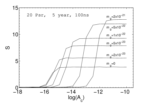
Figure 3.— The expected GW background detection significance using a pulsar timing array with 20 pulsars, observed for 5 years, with 100 ns timing noise. The graviton mass, in units of electron volts, is labeled above each curve. The $x$-axis is the amplitude for the characteristic strain of the GW background ($f_{0}=1\,{\rm yr}^{-1}$, $\alpha=-2/3$), while the $y$-axis is the expected detection significance $S$.

6. Estimate of the Detectability of the Massive Graviton

In § 5, we have discussed how the detection significance for the stochastic GW background is affected by the graviton mass. Here we formulate the qustion as a detection problem rather than a parameter estimation problem. In this section, we will construct a detector, which accepts pulsar timing array data and then determines if the gravitational wave background is massless or massive. Then we simulate pulsar timing data, passing through the detector, to determine the quality of such detector. With the detector quality, we then discusse related technical requirements (the number of pulsars, the pulsar noise level, and so on) for performing such detections.

The question, whether the graviton mass is zero or not, is best formulated as a statistical hypothesis test composed of two hypotheses F and H given by

$$\left\{\begin{array}[]{c}\textrm{H: The graviton is massless;}\\ \textrm{F: The graviton is massive.}\end{array}\right.$$

The detection algorithm determines which hypothesis is accepted. We define the detection rate $P_{\rm d}$ as the probability that the detection algorithm gives statement F, when the graviton is massive, i.e., $P_{\rm d}=P(F|m_{\rm g}>0)$; and we define the false alarm rate $P_{\rm f}$ as the probability of getting statement F when the graviton is massless, i.e., $P_{\rm f}=P(F|m_{\rm g}=0)$. The quality of the detection algorithm is evaluated by calculating the relation between the detection rate $P_{\rm d}$ and the false alarm rate $P_{\rm f}$. Here we take the standard approach (DiFranco & Rubin, 1968) that one fixes $P_{\rm f}$ to a certain threshold level $P_{\rm th}$ and calculates the corresponding $P_{\rm d}$. Throughout this paper we fix $P_{\rm th}=0.1\%$. If a detector maximizes the $P_{\rm d}$ for a prescribed value of $P_{\rm f}$, we say that such detector is optimal (Kassam, 1988).

As we have shown in § 4, the graviton mass changes the shape of the correlation function. The best way to detect such a difference is to use following statistics (Kassam, 1988)

$$\gamma=\frac{\sum_{m=1}^{M}\left(C_{\rm m}(\theta_{m})-\overline{C_{\rm m}}\right)\left(c(\theta_{m})-\overline{c}\right)}{\sqrt{\sum_{m=1}^{M}\left(C_{\rm m}(\theta_{m})-\overline{C_{\rm m}}\right)^{2}\sum_{j=1}^{M}\left(c(\theta_{m})-\overline{c}\right)^{2}}}-\frac{\sum_{m=1}^{M}\left(C_{0}(\theta_{m})-\overline{C_{0}}\right)\left(c(\theta_{m})-\overline{c}\right)}{\sqrt{\sum_{j=1}^{M}\left(C_{0}(\theta_{m})-\overline{C_{0}}\right)^{2}\sum_{j=1}^{M}\left(c(\theta_{m})-\overline{c}\right)^{2}}},$$ (22)

where $C_{0}(\theta)$ is the correlation function for a massless GW background, and $C_{\rm m}(\theta)$ is the correlation function for a massive GW background, which maximizes the detection significance $S$ among possible theoretical correlation functions for all possible values of $m_{\rm g}$. One can show that the optimal statistical decision rule is (Kassam, 1988),

$$\left\{\begin{array}[]{c}\textrm{Choose H: if }\gamma\leq\gamma_{\rm th},\\ \textrm{Choose F: if }\gamma<\gamma_{\rm th},\end{array}\right.$$

where the $\gamma_{\rm th}$ is the threshold of statistical decision, which is determined to guarantee the false alarm rate constraint $P_{\rm f}\leq P_{\rm th}=0.1\%$.

We determine the threshold $\gamma_{\rm th}$ by a third set of Monte-Carlo simulations. These simulations take following steps. First, a massless GW background is generated, then we search for the matched value of $m_{\rm g}$, such that the corresponding correlation function $C_{\rm m}(\theta)$ maximizes the detection significance $S$. Then we use this $C_{\rm m}(\theta)$ to calculate the statistic $\gamma$. We repeat this, recording the values of $\gamma$, to establish the statistical distribution of $\gamma$ values. We take the value of the threshold $\gamma_{\rm th}$ to be that for which there is less than a $0.1\%$ chance of getting $\gamma>\gamma_{\rm th}$ for the case of $m_{\rm g}=0$.

After we determined the $\gamma_{\rm th}$, a fourth Monte-Carlo simulation is used to calculated $P_{\rm d}$. This simulation is very similar to the previous one, except that a massive GW background is generated. We repeat the simulation $10^{3}$ times and take as $P_{\rm d}$ the probability of getting $\gamma>\gamma_{\rm th}$.

We summarize the results of the simulation in Fig. 4, which are gray-scale contour plots for the detection rate $P_{\rm d}$ for different scenarios of using 60, 100, and 300 pulsars respectively. The corresponding parameters are given in the legend of each panel. Intuitively, the necessary conditions for a positive detection of a graviton mass should be first, that the GW is strong enough for the GW to be detected, and second, that the graviton mass is large enough to change the shape of correlation function. This intuition is confirmed by our simulations, which show that the high detection rate concentrates in the upper right corner of each panel, where both graviton mass and GW amplitude are large enough.

From Fig. 4 we can also see that we need at least 60 pulsars to be able to tell the difference between a massive GW background and a massless one. For 5-year observations of 100 pulsars we can start to detect a graviton heavier than $2.5\times 10^{-22}$ eV and we can achieve a limit of $m_{\rm g}=10^{-22}$ eV by using 5-year observations of 300 pulsars. We can achieve levels of $10^{-22}$ eV and $5\times 10^{-23}$ eV in 10-year observations using 100 and 300 puslars respectively.

We also note that there is a positive correlation between the minimal detectable graviton mass and the GW background amplitude, as shown by the leftwards lead edge of the contours, in other words, we need a larger GW amplitude such that the GW background can be detected, if gravitons are more massive. As discussed above, this correlation is due to the reduction of pulsar timing residuals due to massive graviton.

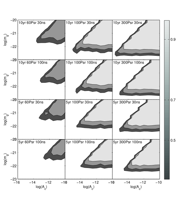
Figure 4.— Contours of 50%, 70 % and 90% detection rates for graviton mass. The white areas are the parameter space for less than 50% detection rate; the light gray regions are the parameter space with more than 90% chance of detecting graviton mass. The false alarm rate is fixed at 0.1% for all calculations. The time span between two successive observation is two weeks. The horizontal axis is the base 10 logarithm of the characteristic strain for the GW background. The vertical axis is the logarithm of graviton mass in unit of eV. The number of pulsars in the timing array, the total time span of observation, and the level of intrinsic pulsar timing noise are given in the legend of each panel. For all the results, we use $\alpha=-2/3$.

7. Conclusion and Discussion

Current efforts to detect gravitational waves using radio pulsar observations make use of correlated arrival time fluctuations induced by the presence of a stochastic GW background. Einstein’s general theory of relativity makes a specific prediction for the angular dependence of the correlation. The power spectrum of the induced fluctuations is given by the power spectrum of the gravitational wave background, determined by the physical processes of the generation process, divided by the square of the GW frequency. In this paper, we showed that the form of the expected correlation function, as well as the power spectrum of the induced timing fluctuations, will be significantly altered if the graviton had a non-zero mass. Only the transverse traceless GW modes were considered in this analysis.

A non-zero graviton mass introduces a cut-off frequency below which no GWs will propagate. If we consider a fixed amount of time over which the correlation will be measured, five years for example, a small increase in the graviton mass will actually increase our ability to detect a strong background. Here, we are assuming that the background is being generated by an ensemble of supermassive black hole binaries. This effect is due to the fact that the presence of the graviton mass will act to flatten out the spectrum of the induced time residuals (see Eq. (15) and Fig. 1), thus making the strong background easier to detect. As the mass is increased, the cut-off frequency will increase. Once this cut-off frequency is above the inverse of the observing time, the sensitivity starts to fall of dramatically. This is due to the fact that pulsar timing is most sensitive to the lowest observable frequencies and the presence of a massive graviton removes all gravitational wave power at frequencies below the cut-off frequency.

A non-zero graviton mass will also change the shape of the angular dependent correlation function. In order to understand this, consider two GW waves traveling near the direction of the line of sight between the Earth and a given pulsar. One GW is traveling towards the pulsar, and the other is traveling towards the Earth. The induced timing fluctuations will be very different for each of these waves. The GW traveling towards the Earth will induce higher amplitude fluctuations then its counter part traveling towards the pulsar. Now, consider the same case but with a massive graviton. As the GW frequency approaches the cut-off frequency, the GW wavelength get arbitrarily large. Assume that the GW wavelength is much larger than the Earth-pulsar distance. In this case, both GWs look exactly the same as far as the Earth-pulsar detector is concerned. Hence, both waves induce the same timing fluctuations. This symmetry between the two GW directions implies that the timing fluctuations from two pulsars near each other on the sky or $180^{\circ}$ apart will have the same amount of correlation, unlike the massless graviton case. Thus, as the graviton mass increases, the correlation curve will become more symmetric about $90^{\circ}$.

Since the graviton mass changes the expected correlation function, we can detect the massive graviton by measuring the shape of correlation function. The optimal detection algorithm differentiating between a massive and a massless GW background was constructed in this paper. Using this algorithm, we found that at least 60 pulsars are required to discriminate between a GW background made up of massive and massless gravitons. Note that, like the case of discriminating various polarization modes of GWs (Lee et al., 2008), the minimum number of pulsars is insensitive to the intrinsic timing noise level or the total observing time.

Here, we are mainly focusing on answering following question: What is the threshold of graviton mass, such that the detector, we constructed in the paper, will find out that the GW background is composed of massive gravitons rather than massless gravitons? We answered this statistical detection question in this paper. The related parameter estimation question will be investigated in the future works.

In this paper, we treat the graviton mass in the sense of a GW dispersion relation. A better graviton mass upper limit ($m_{\rm g}\leq 2\times 10^{-26}$ eV) can be achieved by observing the GW dispersion using Laser Interferometer Space Antenna (LISA) (Stavridis & Will, 2009). Besides GW dispersion based techniques, there are other good upper limits ($2\times 10^{-29}h_{0}$ eV) from galaxy cluster observations (Goldhaber & Nieto, 1974). However since some gravity theories (Maggiore, 2008) contain mass terms for $h_{ab}$, but maintain the scalar sectors, the $m_{\rm g}$ upper limits from GW dispersion observations are independent of the upper limits from Yukawa potential experiments such as the Solar System and the galaxy cluster observations.

In summary, for the task of detecting the massive graviton using a pulsar timing array, there is one critical requirement: a large sample of stable pulsars. Thus the on-going and upcoming projects like the Parkes Pulsar Timing Array (Hobbs et al., 2009b), European Pulsar Timing Array (Stappers et al., 2006), NANOGrav (Jenet et al., 2009), the Large European Array for Pulsars (Stappers et al., 2009), the Five-hundred-meter Aperture Spherical Radio Telescope (Nan et al., 2006; Smits et al., 2009) and the Square Kilometer Array (SKA) will offer unique opportunities to find, to time these pulsars; and to detect the GW background and measure its properties.

8. Acknowledgment

K. J. Lee gratefully acknowledge support from ERC Advanced Grant “LEAP“, Grant Agreement Number 227947 (PI M. Kramer), F. A. Jenet and R. H. Price gratefully acknowledge support from the NSF under grants AST0545837 and PHY0554367, and support from the UTB Center for Gravitational Wave Astronomy. We also thank M. Pshirkov and N. Straumann for very useful comments.

Appendix A Power spectra of timing residual

The power spectra of timing residuals is calculated by integrating Eq. (14). Here we give the details of the calculation.

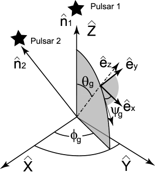
Figure 5.— The geometric configuration of the coordinates and unit vectors used here. The $\hat{X}$, $\hat{Y}$ and $\hat{Z}$ are the coordinate unit vectors, ${\hat{\rm\bf e}_{z}\,\!}$ is the propagation direction of the GW, and $\hat{\rm\bf n}_{1}$ and $\hat{\rm\bf n}_{2}$ are unit vectors pointing to the pulsars.

In Fig. 5, the components of ${\hat{\rm\bf e}_{z}\,\!}$ in the $\hat{\bf X}^{a}=(\hat{\bf X},\hat{\bf Y},\hat{\bf Z})$ frame can be seen to be $(\sin\theta_{g}\cos\phi_{g},$ $\sin\theta_{g}\sin\phi_{g},\cos\theta_{g})$, where the $\theta_{g}$ and $\phi_{g}$ are respectively the polar angle and azimuthal angle of the GW propagation vector. To proceed, we need the components of the polarization tensors in the $\hat{\bf X}^{a}$ frame. The transformation from the components ${\epsilon}_{0,cd}$ given in the GW frame $\hat{\bf e}_{b}=(\hat{\bf e}_{x},\hat{\bf e}_{y},\hat{\bf e}_{z})$ of Eq. (4) is made with ${\epsilon}^{P}_{ab}=T_{ca}T_{db}\,{\epsilon}^{P}_{0,cd}$, where $T_{ca}=\hat{\bf e}_{c}\cdot\hat{\bf X}_{a}$ has components

$$\left({\begin{array}[]{c c c}\cos\theta_{g}\cos\phi_{g}\cos{\psi_{g}}-\sin\phi_{g}\sin{\psi_{g}}&\cos\theta_{g}\cos\psi_{g}\sin\phi_{g}+\cos\phi_{g}\sin\psi_{g}&-\cos\psi_{g}\sin\theta_{g}\\ -\cos\psi_{g}\sin\phi_{g}-\cos\theta_{g}\cos\phi_{g}\sin\psi_{g}&\cos\phi_{g}\cos\psi_{g}-\cos\theta_{g}\sin\phi_{g}\sin\psi_{g}&\sin\theta_{g}\sin\psi_{g}\\ \cos\phi_{g}\sin\theta_{g}&\sin\theta_{g}\sin\phi_{g}&\cos\theta_{g}\end{array}}\right)\,.$$ (A1)

Since the GW background is isotropic, with no loss of generality one can choose $\hat{\rm\bf n}=\{0,0,1\}$ so that

$${\omega_{\rm g}}+c\hat{\rm\bf n}\cdot{\rm\bf{k_{\rm g}}}=(1+\zeta\cos\theta_{\rm g})\,{\omega_{\rm g}},$$ (A2)

where

$$\zeta=\sqrt{1-\frac{{m_{\rm g}}^{2}c^{4}}{{\omega_{\rm g}}^{2}\hbar^{2}}\;}=\sqrt{1-\frac{f_{\rm cut}^{2}}{f_{\rm g}^{2}}\;}\,,$$ (A3)

for $f_{\rm g}\geq f_{\rm cut}$ . The term ${\epsilon}^{P}_{ij}\hat{\rm\bf n}^{i}\hat{\rm\bf n}^{j}$ now simplifies to

$${\epsilon}^{+}_{ij}\hat{\rm\bf n}^{i}\hat{\rm\bf n}^{j} = \sin^{2}\theta_{\rm g}\cos(2\psi_{\rm g})$$

$${\epsilon}^{\times}_{ij}\hat{\rm\bf n}^{i}\hat{\rm\bf n}^{j} = -\sin^{2}\theta_{\rm g}\sin(2\psi_{\rm g})\,.$$ (A4)

After the ensemble average over the polarization angle $\psi_{\rm g}$, the integration of Eq. (14) gives

$$S_{\rm R}(f_{\rm g})=\sum_{P=+,\times}\frac{|h_{c}^{P}(f_{\rm g})|^{2}}{128\pi^{3}f_{\rm g}^{3}}\int_{0}^{\pi}d\theta_{\rm g}\int_{0}^{2\pi}d\phi_{\rm g}\frac{\sin^{5}\theta_{\rm g}}{(1+\zeta\cos\theta_{\rm g})^{2}}\left[1-\cos\left(\frac{D{\omega_{\rm g}}}{c}(1+\zeta\cos\theta_{\rm g})\right)\right]$$ (A5)

For practical pulsar timing array, we have $\Phi_{0}=D{\omega_{\rm g}}/c\gg 1$, i.e. , the GW wave length is much smaller than the pulsar-earth distance, so one gets

$$\int_{-1}^{1}\frac{(1-\mu^{2})^{2}}{(1+\zeta\mu)^{2}}\left[1-\cos\left(\Phi_{0}(1+\zeta\mu)\right)\right]d\mu=\frac{4\left[-4\zeta^{3}+6\zeta+3\left(\zeta^{2}-1\right)\log\left(\frac{\zeta+1}{1-\zeta}\right)\right]}{3\zeta^{5}}+O\left(\Phi_{0}^{-2}\right).$$ (A6)

Finally, the power spectra of the pulsar timing residuals then becomes

$$S_{\rm R}(f_{\rm g})=\sum_{P=+,\times}\frac{|h_{c}^{P}(f_{\rm g})|^{2}}{24\pi^{2}f_{\rm g}^{3}}\eta(f_{\rm g})\,.$$ (A7)

For $f_{\rm g}>f_{\rm cut}$, $\eta$ is given by

$$\eta(f_{\rm g})=\frac{-4\zeta^{3}+6\zeta+3\left(\zeta^{2}-1\right)\log\left(\frac{\zeta+1}{1-\zeta}\right)}{2\zeta^{5}}\,,$$ (A8)

with $\zeta$ is given by Eq. (A3) . For $f_{\rm g}\leq f_{\rm cut}$ the gravitational waves cannot propagate, and we take $\eta=0$.

Appendix B Angular Dependent Correlation Function for Pulsar Timing Residuals

The correlation function $C(\theta)$ between pulsar ‘$a$’ and ‘$b$’ defined in this paper is

$$C(\theta)=\frac{\langle R_{a}(t)R_{b}(t)\rangle}{\sigma_{a}\sigma_{b}},$$ (B1)

where $\theta$ is the angle between the direction to pulsar ‘$a$’ and the direction to pulsar ‘$b$’. The $R_{a}(t)$ and $R_{b}(t)$ are the GW induced timing residuals for pulsar ‘$a$’ and ‘$b$’ respectively. The $\sigma_{a}$ and $\sigma_{b}$ are the RMS value for the timing residual $R_{a}(t)$ and $R_{b}(t)$. One has (see Lee et al. (2008) for a similar calculation)

$$C(\theta)=\frac{1}{\sigma_{a}\sigma_{b}}\sum_{P=+,\times}\left\langle\int_{0}^{\infty}\frac{|h_{c}^{P}(f_{\rm g})|^{2}}{64\pi f_{\rm g}}df_{\rm g}\int d\Omega\frac{{\epsilon}^{P}_{ij}\hat{\rm\bf n}_{a}^{i}\hat{\rm\bf n}_{a}^{j}}{{\omega_{\rm g}}+c{\rm\bf{k_{\rm g}}\cdot\hat{\rm\bf n}_{a}}}\frac{{\epsilon}^{P}_{ij}\hat{\rm\bf n}_{b}^{i}\hat{\rm\bf n}_{b}^{j}}{{\omega_{\rm g}}+c{\rm\bf{k_{\rm g}}\cdot\hat{\rm\bf n}_{b}}}{\cal P}_{ab}\right\rangle,$$ (B2)

where ${\cal P}_{ab}$ is given by

$${\cal P}_{ab} = 1-\cos\Phi_{a}-\cos\Phi_{b}+\cos(\Phi_{a}-\Phi_{b});$$

$$\Phi_{a} = \frac{D_{a}}{c}({\omega_{\rm g}}+c{k_{\rm g}}\cdot\hat{\rm\bf n}_{a});$$

$$\Phi_{b} = \frac{D_{b}}{c}({\omega_{\rm g}}+c{k_{\rm g}}\cdot\hat{\rm\bf n}_{b}).$$ (B3)

Equation (B2) shows that the correlation function is composed of two major integrations, one over the GW frequency $df_{\rm g}$, and the one over solid angle $d\Omega$. For the massless graviton case, these two parts are not mixed, since ${k_{\rm g}}$ is linear in ${\omega_{\rm g}}$. But ${k_{\rm g}}$ is non-linear in ${\omega_{\rm g}}$ for the case of a massive graviton. The nonlinear dependence in Eq. (2) mixes the spatial integral with the frequency one. Thus the shape of $C(\theta)$ depends on both the graviton mass and the frequency spectra of GWs, which also depends on the observation schedule. Thus, it is unlikely that one can integrate Eq. (B2) analytically.

References

- Alves et al. (2009) Alves, M. E. S., Miranda, O. D., & de Araujo, J. C. N. 2010, CQG,27, 145010
- Anderson et al. (2008) Anderson, J. D., Campbell, J. K., Ekelund, J. E., Ellis, J., & Jordan, J. F. 2008, Physical Review Letters, 100, 091102
- Anderson et al. (1998) Anderson, J. D., Laing, P. A., Lau, E. L., Liu, A. S., Nieto, M. M., & Turyshev, S. G. 1998, Physical Review Letters, 81, 2858
- Arnowitt & Deser (1959) Arnowitt, R., & Deser, S. 1959, Physical Review, 113, 745
- Baskaran et al. (2008a) Baskaran, D., Polnarev, A. G., Pshirkov, M. S., & Postnov, K. A. 2008a, Phys. Rev. D, 78, 089901
- Baskaran et al. (2008b) —. 2008b, Phys. Rev. D, 78, 044018
- Choudhury et al. (2004) Choudhury, S. R., Joshi, G. C., Mahajan, S., & McKellar, B. H. J. 2004, Astroparticle Physics, 21, 559
- Cutler et al. (2003) Cutler, C., Hiscock, W. A., & Larson, S. L. 2003, Phys. Rev. D, 67, 024015
- Damour (2007) Damour, T. 2007, A Century from Einstein Relativity: Probing Gravity Theories in Binary Systems: Binary Systems as Test-beds of Gravity Theories, ed. M. Colpi (Springer)
- Damour et al. (2003) Damour, T., Kogan, I. I., & Papazoglou, A. 2003, Phys. Rev. D, 67, 064009
- Deffayet et al. (2002) Deffayet, C., Dvali, G., Gabadadze, G., & Vainshtein, A. 2002, Phys. Rev. D, 65, 044026
- Detweiler (1979) Detweiler, S. 1979, ApJ, 234, 1100
- DiFranco & Rubin (1968) DiFranco, J. V., & Rubin, W. L. 1968, Radar Detection, ed. W. L. Everitt, Prentice-Hall Electrical Engineering Series (Prentice-Hall INC)
- Dvali et al. (2000) Dvali, G., Gabadadze, G., & Porrati, M. 2000, Physics Letters B, 485, 208
- Eckhardt et al. (2010) Eckhardt, D. H., Pestaña, J. L. G., & Fischbach, E. 2010, New Astronomy, 15, 175
- Enoki et al. (2004) Enoki, M., Inoue, K. T., Nagashima, M., & Sugiyama, N. 2004, ApJ, 615, 19
- Estabrook & Wahlquist (1975) Estabrook, F. B., & Wahlquist, H. D. 1975, General Relativity and Gravitation, 6, 439
- Finn & Sutton (2002) Finn, L. S., & Sutton, P. J. 2002, Phys. Rev. D, 65, 044022
- Goldhaber & Nieto (1974) Goldhaber, A. S., & Nieto, M. M. 1974, Phys. Rev. D, 9, 1119
- Goldhaber & Nieto (2010) —. 2010, Reviews of Modern Physics, 82, 939
- Gupta (1952) Gupta, S. N. 1952, Proceedings of the Physical Society A, 65, 161
- Hare (1973) Hare, M. G. 1973, Canadian Journal of Physics, 51, 431
- Hellings & Downs (1983) Hellings, R. W., & Downs, G. S. 1983, ApJ, 265, L39
- Hobbs et al. (2009a) Hobbs, G., Jenet, F., Lee, K. J., Verbiest, J. P. W., Yardley, D., Manchester, R., Lommen, A., Coles, W., Edwards, R., & Shettigara, C. 2009a, MNRAS, 394, 1945
- Hobbs et al. (2009b) Hobbs, G. B., Bailes, M., Bhat, N. D. R., Burke-Spolaor, S., Champion, D. J., Coles, W., Hotan, A., Jenet, F., Kedziora-Chudczer, L., Khoo, J., Lee, K. J., Lommen, A., Manchester, R. N., Reynolds, J., Sarkissian, J., van Straten, W., To, S., Verbiest, J. P. W., Yardley, D., & You, X. P. 2009b, Publications of the Astronomical Society of Australia, 26, 103
- Hough & Rowan (2000) Hough, J., & Rowan, S. 2000, Living Reviews in Relativity, 3, 3
- Hough et al. (2005) Hough, J., Rowan, S., & Sathyaprakash, B. S. 2005, Journal of Physics B Atomic Molecular Physics, 38, 497
- Iwasaki (1970) Iwasaki, Y. 1970, Phys. Rev. D, 2, 2255
- Jaffe & Backer (2003) Jaffe, A. H., & Backer, D. C. 2003, ApJ, 583, 616
- Jenet et al. (2009) Jenet, F., Finn, L. S., Lazio, J., Lommen, A., McLaughlin, M., Stairs, I., Stinebring, D., Verbiest, J., Archibald, A., Arzoumanian, Z., Backer, D., Cordes, J., Demorest, P., Ferdman, R., Freire, P., Gonzalez, M., Kaspi, V., Kondratiev, V., Lorimer, D., Lynch, R., Nice, D., Ransom, S., Shannon, R., & Siemens, X. 2009, Preprint, arxiv: 09091058
- Jenet et al. (2005) Jenet, F. A., Hobbs, G. B., Lee, K. J., & Manchester, R. N. 2005, ApJ, 625, L123
- Kassam (1988) Kassam, S. A. 1988, Signal Detection in Non-Gaussian Noise (New York: Springer Verlag)
- Kiefer (2006) Kiefer, C. 2006, Annalen der Physik, 15, 129
- Kramer & Wex (2009) Kramer, M., & Wex, N. 2009, Classical and Quantum Gravity, 26, 073001
- Landau & Lifshitz (1960) Landau, L. D., & Lifshitz, E. M. 1960, Electrodynamics of continuous media (Oxford: Pergamon Press)
- Larson & Hiscock (2000) Larson, S. L., & Hiscock, W. A. 2000, Phys. Rev. D, 61, 104008
- Lee et al. (2008) Lee, K. J., Jenet, F. A., & Price, R. H. 2008, ApJ, 685, 1304
- Liang (2000) Liang, C. B. 2000, Introduction of differential geometry and general relativity (in Chinese), Vol. V1 (Beijing: Publisher of Beijing Normal University)
- Maggiore (2000) Maggiore, M. 2000, Phys. Rep., 331, 283
- Maggiore (2008) —. 2008, Gravitational waves, Vol. V1 (Oxford: Oxford University Press)
- Manchester (2006) Manchester, R. N. 2006, Chinese Journal of Astronomy and Astrophysics Supplement, 6, 020000
- Nan et al. (2006) Nan, R., Wang, Q., Zhu, L., Zhu, W., Jin, C., & Gan, H. 2006, Chinese Journal of Astronomy and Astrophysics Supplement, 6, 020000
- Particle Data Group (2008) Particle Data Group. 2008, Physics Letters B, 667, 1
- Phinney (2001) Phinney, E. S. 2001, preprint, arxiv: 0108028
- Rubakov & Tinyakov (2008) Rubakov, V. A., & Tinyakov, P. G. 2008, Physics Uspekhi, 51, 759
- Sallmen et al. (1993) Sallmen, S., Backer, D. C., & Foster, R. 1993, in Bulletin of the American Astronomical Society, Vol. 25, Bulletin of the American Astronomical Society, 853
- Sanders & McGaugh (2002) Sanders, R. H., & McGaugh, S. S. 2002, ARA&A, 40, 263
- Sazhin (1978) Sazhin, M. V. 1978, Soviet Astronomy, 22, 36
- Sesana et al. (2004) Sesana, A., Haardt, F., Madau, P., & Volonteri, M. 2004, ApJ, 611, 623
- Smits et al. (2009) Smits, R., Lorimer, D. R., Kramer, M., Manchester, R., Stappers, B., Jin, C. J., Nan, R. D., & Li, D. 2009, A&A, 505, 919
- Smolin (2003) Smolin, L. 2003, arXiv:hep-th/0303185
- Stairs (2003) Stairs, I. H. 2003, Living Reviews in Relativity, 6, 5
- Stappers et al. (2009) Stappers, B., Vlemmings, W., & Kramer, M. 2009, Proceedings of Science, EXPReS09, 20
- Stappers et al. (2006) Stappers, B. W., Kramer, M., Lyne, A. G., D’Amico, N., & Jessner, A. 2006, Chinese Journal of Astronomy and Astrophysics Supplement, 6, 020000
- Stavridis & Will (2009) Stavridis, A., & Will, C. M. 2009, Phys. Rev. D, 80, 044002
- Vainshtein (1972) Vainshtein, A. I. 1972, Physics Letters B, 39, 393
- van Dam & Veltman (1970) van Dam, H., & Veltman, M. 1970, Nuclear Physics B, 22, 397
- Visser (1998) Visser, M. 1998, General Relativity and Gravitation, 30, 1717
- Weinberg (1972) Weinberg, S. 1972, Gravitation and Cosmology: Principles and Applications of the General Theory of Relativity (John Wiley & Sons)
- Wen et al. (2009) Wen, Z. L., Liu, F. S., & Han, J. L. 2009, ApJ, 692, 511
- Will (2006) Will, C. 2006, Living Reviews in Relativity, 9, 3
- Will (1993) Will, C. M. 1993, Theory and Experiment in Gravitational Physics (UK: Cambridge University Press)
- Will (1998) —. 1998, Phys. Rev. D, 57, 2061
- Wyithe & Loeb (2003) Wyithe, J. S. B., & Loeb, A. 2003, ApJ, 590, 691
- Zakharov (1970) Zakharov, V. I. 1970, JETP, 12,312