Quantization of FRW universe via gauge-fixed action

Abstract

This paper is devoted to investigation of the quantum Friedman-Robertson-Walker universe with matter satisfying the equation of state $p=w\rho$, where $w$ is an almost arbitrary constant. The procedure starts with a reduced Lagrangian, which describes the system in a gauge fixed, so that the evolution parameter corresponds to the cosmological time. Then we construct the phase space, which is believed to correspond to the reduced phase space consisting of Dirac’s observables. The physically relevant quantities are mapped into operators. We show that the operators have self-adjoint realizations and that there exist quantum states for which the evolution across singularity is well-defined.

I Introduction

For a gauge system like general relativity, there exist two ways of quantizing. (i) The Dirac method PAM starts with quantization of all the degrees of freedom of the configuration space of e.g. the Hilbert-Einstein action. Then the gauge freedom is removed from the quantum theory by solving the constraint operator equation. On the other hand, (ii) the reduced phase space method (see e.g. Mal ) begins with canonical formulation of the classical theory and then the gauge freedom is removed by identification of all Dirac’s observables through the following weak equality: $\{C,\Omega\}\approx 0$, where $C$ is a constraint, $\Omega$ is a Dirac’s observable and the equality is weak in the sense that it holds on the constraint surface $C=0$ (it excludes the solutions of the type $\Omega=C$). Then the Dirac observables, which are physical degrees of freedom, are mapped into quantum operators.

In this paper we take yet another route: we remove the gauge freedom already at the level of Lagrangian. Then we move to a Hamiltonian formulation and subsequently we quantize the canonical system using the Schrödinger representation. The analysis is restricted to the compact, flat FRW universe.

In section II, starting with a given Lagrangian, we show that it describes the system under consideration and arrive at canonical formulation in convenient basic variables. In section III, we map the phase space functions into operators and study their self-adjointness. Next, in section IV we compute the evolution of mean values of the relevant operators. We conclude in section V.

In appendix A we make conjecture that the reduced phase space method is closely related to the reduced Lagrangian method.

In appendix B we report on an unsuccessful attempt at resolving the singularity. It is discussed and compared with approach used throughout this paper in concluding section V.

II Classical theory

The metric of the flat FRW universe in the comoving coordinates and with respect to the cosmological time $t$ reads:

$$ds^{2}=-dt^{2}+a(t)^{2}d\overline{x}^{2},$$ (1)

where $a(t)$ is a scale factor and $d\overline{x}$ is a distance measure in a space-like leaf $\Sigma$. Instead of the scale factor $a$, we are going to consider the dynamics of the physical length between two unspecified points in $\Sigma$ and we denote it by $l(t):=l_{0}\frac{a(t)}{a(t_{0})}$, where $l_{0}$ is the length at the moment $t=t_{0}$. Therefore, for each value of $t$, the length $l(t)$ is a physical quantity, i.e. the Dirac observable. Now let us see how one can introduce the dynamics of $l$.

II.1 Lagrangian formulation

Let us examine the following action integral:

$$S=\int\mathbb{L}(l,\dot{l})~{}dt=\alpha\int l^{3w+1}\dot{l}^{2}~{}dt,$$ (2)

where $\alpha:=\frac{3}{8\pi G}\cdot\frac{1}{\lambda^{3w}}$ and $\lambda$ is a constant of the length dimension and will be specified later. The parameter $w$ is a real constant. Variation with respect to $l$ gives the equation of motion:

$$-(3w+1)\alpha l^{3w}\dot{l}^{2}-2\alpha l^{3w+1}\ddot{l}=0=\bigg{(}l^{\frac{3w+3}{2}}\bigg{)},_{tt},$$ (3)

which has the solutions:

$$l(t)=l_{0}\bigg{(}\frac{3w+3}{2}\frac{\dot{l}_{0}}{l_{0}}(t-t_{0})+1\bigg{)}^{\frac{2}{3w+3}},$$ (4)

satisfying the initial conditions:

$$l(t_{0})=l_{0},~{}~{}~{}~{}\dot{l}(t_{0})=\dot{l}_{0}.$$ (5)

Let us turn to the Friedman equations:

$$H^{2} = \frac{8\pi G}{3}\rho,$$ (6)

$$H^{2}+\dot{H} = -\frac{4\pi G}{3}(\rho+3p),$$ (7)

where $H$ is Hubble’s parameter, $\rho$ is the energy density and $p$ is the pressure of the matter in the universe. Now, making use of $H:=\frac{\dot{l}}{l}$, we find out that:

$$H^{2}=(\dot{l}_{0}^{2}l_{0}^{3w+1})\frac{1}{l^{3w+3}},~{}~{}~{}~{}H^{2}+\dot{H}=-\frac{1}{2}(1+3w)(\dot{l}_{0}^{2}l_{0}^{3w+1})\frac{1}{l^{3w+3}},$$ (8)

and we easily conclude that our system given by the action integral (2) is the flat FRW universe with $\frac{8\pi G}{3}\rho=(\dot{l}_{0}^{2}l_{0}^{3w+1})\frac{1}{l^{3w+3}}$ and $p=w\rho$.

Hence, we have succeeded in the gauge-fixed Lagrangian formulation of the dynamics of the flat FRW universe filled with matter satisfying the equation of state $p=w\rho$. The connection of this reduced Lagrangian with the reduced phase space procedure, which begins with the introduction of the kinematical phase space (consisting of both gauge and physical degrees of freedom), is commented in appendix A.

The energy of matter contained in a fiducial cubic cell of the edge length changing with time as $l(t)$, reads:

$$E_{matt}=\frac{3l_{0}^{3}}{8\pi G}\bigg{(}\frac{\dot{l}_{0}}{l_{0}}\bigg{)}^{2}\bigg{(}\frac{l}{l_{0}}\bigg{)}^{-3w},$$ (9)

and, for $w\neq 0$, is clearly not conserved. For instance, the matter may consist of particles, which move with respect to the comoving reference frame, then the particles loose/gain their kinetic energy as the spacetime expands/shrinks and the energy of matter changes with the evolution of the universe. However, one may introduce a conserved quantity, the total energy:

$$E_{tot}=\frac{1}{\lambda^{3w}}\rho\cdot l^{3w+3},$$ (10)

which is equal to the energy of matter at the moment when the value of the length of the fiducial cubic cell is equal to $\lambda$. If the moment happens to be $t=t_{0}$, then $E_{tot}=E_{matt}(t_{0})=\frac{3l_{0}^{3}}{8\pi G}\big{(}\frac{\dot{l}_{0}}{l_{0}}\big{)}^{2}$, and $\lambda=l_{0}$.

II.2 Canonical formulation

We perform the Legendre transformation:

$$l\mapsto l\in\mathbb{R}_{+},~{}~{}~{}~{}\dot{l}\mapsto p_{l}:=\frac{\mathrm{d}\mathbb{L}}{\mathrm{d}\dot{l}}=2\alpha l^{3w+1}\dot{l}\in\mathbb{R},$$ (11)

so that

$$\mathbb{H}=p_{l}\dot{l}-\mathbb{L}=\frac{p_{l}^{2}}{4\alpha l^{3w+1}}~{}~{}~{}~{}\textrm{and}~{}~{}~{}~{}\{l,p_{l}\}=1$$ (12)

Hamilton’s equations:

$$\dot{l}=\{l,\mathbb{H}\}=\frac{p_{l}}{2\alpha l^{3w+1}},~{}~{}~{}~{}\dot{p}_{l}=\{p_{l},\mathbb{H}\}=(3w+1)\frac{p_{l}^{2}}{4\alpha l^{3w+2}}.$$ (13)

can be integrated and we obtain:

$$p_{l}=Cl^{\frac{3w+1}{2}},~{}~{}\textrm{or}~{}~{}p_{l}=0,~{}l=C~{}\textrm{(stationary universe)},$$ (14)

where $C$ is any real constant. The solutions split into three cases: $w<-1/3$, $w=-1/3$ and $w>-1/3$. They respectively correspond to the momentum of space blowing up, being constant and vanishing as the universe approaches the singularity $l=0$.

We are going to study physically interesting quantities like Hubble’s parameter or energy density, which take the following form, respectively:

$$H=\frac{p_{l}}{2\alpha l^{3w+2}},~{}~{}~{}~{}\rho=\frac{3}{8\pi G}H^{2}.$$ (15)

The Hamiltonian $\mathbb{H}$ is a conserved quantity like the total energy of the system defined in eq. (10). The comparison of these two leads to the condition:

$$\frac{1}{\alpha}\frac{p_{l}^{2}}{4l^{3w+1}}=\mathbb{H}=E_{tot}=\frac{1}{\alpha^{2}}\frac{3}{8\pi G}\frac{p_{l}^{2}}{4l^{3w+1}}\frac{1}{\lambda^{3w}},$$ (16)

and hence

$$\alpha=\frac{3}{8\pi G\lambda^{3w}},$$ (17)

which is in accordance with our prior definition and explains the physical meaning of $\lambda$.

II.3 Canonical transformation

In what follows we will look for a more convenient conjugate pair. We assume that:

1. the canonical transformation is valid globally

2. the ’stationary universes’ in (14) are included in the system and thus well-mapped by the transformation

3. canonical transformation does not extend the phase space, in particular it preserves the topology of the phase space under consideration

Now, let us break the above rules in the following example:

$$\{l,p_{l}\}\longrightarrow\{\tilde{l}:=\mathbb{H},\tilde{p}_{l}:=\frac{2H^{-1}}{3(w+1)}\}~{},~{}~{}w\neq-1.$$ (18)

The map is singular for $p_{l}=0$ and thus the ’stationary universes’ being the points at the axis $p_{l}=0$, are excluded now. Instead, the closure of the range of the map covers a new region of the space of parameters, $\tilde{p}_{l}=0$. As a consequence, the trajectories in the phase space are complete and the singularities are absent! But this is not a good way to resolve the singularity, since, apart from the lack of quantum physics, the procedure has a drawback in that it is non-unique and here are further examples:

$$\{l,p_{l}\}\longrightarrow\{\tilde{l}:=\mathbb{H},\tilde{p}_{l}:=\frac{2H^{-1}}{3(w+1)}+\textrm{sgn}(p_{l})f(\mathbb{H})\}~{},~{}~{}w\neq-1,~{}~{}f~{}\textrm{arbitrary}.$$ (19)

Therefore, making use of a ‘regular’ map, we introduce the following new canonical pair:

$$\{l,p_{l}\}\longrightarrow\{\tilde{l}:=\frac{4}{3w+3}l^{(3w+3)/2},\tilde{p}_{l}:=\frac{p_{l}}{2l^{(3w+1)/2}}\}~{},~{}~{}w\neq-1.$$ (20)

Now, the Hamiltonian reads:

$$\mathbb{H}=\frac{1}{\alpha}\tilde{p}_{l}^{2},$$ (21)

the Hubble parameter:

$$H=\frac{1}{\alpha}\frac{4}{3w+3}\frac{\tilde{p}_{l}}{\tilde{l}},$$ (22)

the energy density:

$$\rho=\frac{1}{\alpha^{2}}\frac{2}{\pi G(3w+1)}\frac{\tilde{p}_{l}^{2}}{\tilde{l}^{2}},$$ (23)

and the length:

$$l=\big{(}{\frac{3w+3}{4}~{}\tilde{l}}\big{)}^{2/(3w+3)}.$$ (24)

III Schrödinger quantization

In the Schrödinger representation:

$$\tilde{l}\mapsto\hat{l}:=x,~{}~{}~{}~{}\tilde{p}_{l}\mapsto\hat{p}_{l}:=-i\hbar\frac{d}{dx},$$ (25)

and we get the following formally self-adjoint operators that are relevant in the cosmological context and will be studied below:

$$\mathbb{H}\mapsto\hat{\mathbb{H}}=-\frac{\hbar^{2}}{\alpha}\frac{d^{2}}{dx^{2}},$$ (26)

$$H\mapsto\hat{H}=\frac{\hbar}{\alpha}\frac{4}{3w+3}(-i\frac{d}{dx}x^{-1}-ix^{-1}\frac{d}{dx}),$$ (27)

$$\rho\mapsto\hat{\rho}=\frac{\hbar^{2}}{\alpha^{2}}\frac{1}{2\pi G(3w+1)}(-i\frac{d}{dx}x^{-1}-ix^{-1}\frac{d}{dx})^{2},$$ (28)

$$l\mapsto\hat{l}=\big{(}{\frac{3w+3}{4}x}\big{)}^{2/(3w+3)}.$$ (29)

The range of $x$ is $(0,\infty)$. Thus, the problem of evolution across singularity is formulated in terms of a freely moving quantum particle on a half-line.

III.1 Hamiltonian and the evolution

The theory of the operator $-\frac{d^{2}}{dx^{2}}$ on half-line may be found in Der . In short, there are infinitely many ways, in which one may define the operator $\hat{\mathbb{H}}$ to be essentially self-adjoint on $L^{2}(R_{+},dx)$ and we will denote these options by $\hat{\mathbb{H}}_{\mu}$ for $\mu\in\mathbb{R}\cup\{\infty\}$. In order to calculate the evolution of a given state one may apply the appropriate Fourier Transform, denoted by $FT^{\mu}$, and multiply the resultant wave-function by $e^{-ik^{2}t}$, where $k$ is the momentum.

The important point to be made here is that we do introduce an evolution operator. In the quantization scheme proposed in Mal , one only quantizes the Dirac observables enumerated by a classical evolution parameter - one does not introduce a generator of change in this parameter, called the true Hamiltonian, in order to quantize it. However, in our model of universe this approach would not work - it would not give any sensible solution to the singularity problem. The crucial difference is that in the model presented in Mal the classical dynamics was already non-singular, whereas in the model considered here the dynamics ends at the point $l=0$.

The quantization of the evolution may give some hopes to resolve the singularity. The following heuristic argument shows that the closer to the singularity the more the quantum universe departures from the classical one:

$$\{H,\mathbb{H}\} \sim -2H^{2},$$ (30)

$$\frac{1}{i}[\hat{H},\hat{\mathbb{H}}] \sim -2\hat{H}^{2}+\frac{1}{2}x^{-4}.$$ (31)

We observe that at the classical level (30) the value of the Hubble parameter $H$ goes to minus infinity as the universe approaches the singularity, whereas at the quantum level (31) the term $x^{-4}$ opposes the unbounded decrease of the operator $\hat{H}$. From the form of $\hat{H}$ given in (27), one sees that the ‘closer’ the wave-function to $x=0$, the bigger the value of $\hat{H}^{2}$. But at the same time, the closer the wave-function to $x=0$, the bigger the value of the opposing term $x^{-4}$.

III.2 The energy density and Hubble operators

We will study the formally self-adjoint Hubble operator:

$$\hat{H}=\frac{4}{3w+3}\frac{\hbar}{\alpha}(-i\frac{d}{dx}x^{-1}-ix^{-1}\frac{d}{dx}).$$ (32)

Let us consider the following inverse mapping $L^{2}(\mathbb{R}_{+},dx)\mapsto L^{2}(\mathbb{R}_{+},dy)$:

$$\psi(x)\mapsto\phi(y):=\frac{\psi(2\sqrt{y})}{y^{1/4}},~{}~{}y>0.$$ (33)

Let us see that this mapping is isometric, and hence unitary:

$$\int_{0}^{\infty}\overline{\psi}(x)\psi(x)~{}dx=\int_{0}^{\infty}\overline{\psi}(2\sqrt{y})\psi(2\sqrt{y})~{}2d\sqrt{y}=\int_{0}^{\infty}\frac{\overline{\psi}(2\sqrt{y})}{y^{1/4}}\frac{\psi(2\sqrt{y})}{y^{1/4}}~{}dy.$$ (34)

Application of the mapping (33) to the operator $\hat{H}$ gives:

$$\frac{-4i}{3w+3}\frac{\hbar}{\alpha}y^{-1/4}(-x^{-2}+2x^{-1}\frac{d}{dx})y^{1/4}=\frac{-4i}{3w+3}\frac{\hbar}{\alpha}\frac{d}{dy},$$ (35)

which is a simple derivative operator. Analogically, under the same mapping the energy density operator $\hat{\rho}$ is transformed into Laplacian $\sim-\frac{d^{2}}{dy^{2}}$.

Again, there are infinitely many inequivalent ways, in which one may define a self-adjoint $\hat{\rho}$, and we will denote these options by $\hat{\rho}_{\mu},~{}\mu\in\mathbb{R}\cup\{\infty\}$. However, the Hubble operator, being a momentum operator, cannot be self-adjoint on the half-line. Therefore, we will redefine $\hat{H}:=\sqrt{\hat{\rho}}$. The spectrum of these operators reads $sp(\hat{\rho}_{\mu})=sp(\hat{H}_{\mu})=\mathbb{R}_{+}$ for any $\mu$.

III.3 The volume operator

The volume operator $\hat{v}:=\hat{l}^{3}=\big{(}{\frac{3w+3}{4}x}\big{)}^{2/(w+1)}$ is a self-adjoint operator on $L^{2}(\mathbb{R}_{+},dx)$ and its spectrum for $w>-1$ reads $sp(\hat{v})=\mathbb{R}_{+}$.

IV Evolution of physical quantities

Let us restrict to the study of the evolution that preserves the Dirichlet condition (i.e. generated by $\hat{\mathbb{H}}_{\mu}$ for $\mu=\infty$). We pick the following family of wave-functions:

$$\tilde{\phi}_{a}(k):=Nke^{-ak^{2}},~{}~{}k>0,$$ (36)

where $N=2\frac{(2a)^{3/4}}{\pi^{1/4}}$, $[k]=[x]^{-1}=m^{-\frac{3w+3}{2}}$, $[a]=m^{3w+3}$ and evolve them in time:

$$\exp{(-\frac{i}{\hbar}t\hat{\mathbb{H}})}\tilde{\phi}_{a}(k)=\exp{(-i\frac{\hbar}{\alpha}tk^{2})}\tilde{\phi}_{a}(k)=Nke^{-(a+i\frac{\hbar}{\alpha}t)k^{2}}=\tilde{\phi}_{a}(k,t).$$ (37)

Applying the Fourier sine transform $FT^{\infty}$ renders:

$$\phi_{a}(x,t):=\int_{0}^{\infty}\sin(kx)\tilde{\phi}_{a}(k,t)dk=\frac{Nx}{(2(a+i\frac{\hbar}{\alpha}t))^{3/2}}~{}e^{-\frac{x^{2}}{4(a+i\frac{\hbar}{\alpha}t)}}.$$ (38)

IV.1 The invariant $\sqrt[w+1]{E_{tot}}$

Let us calculate the expectation value of the operator corresponding to the classical invariant $\sqrt[w+1]{E_{tot}}$ :

$$\langle\sqrt[w+1]{E_{tot}}~{}\rangle:=\langle\tilde{\phi}_{a}(k)|\sqrt[w+1]{\hat{\mathbb{H}}}~{}\tilde{\phi}_{a}(k)\rangle=\sqrt[w+1]{\frac{\hbar^{2}}{\alpha}}|N|^{2}\int_{0}^{\infty}e^{-2ak^{2}}k^{\frac{2w+4}{w+1}}~{}dk$$

$$=\sqrt[w+1]{\frac{\hbar^{2}}{2\alpha}\bigg{(}\frac{2}{\sqrt{\pi}}\Gamma\bigg{(}\frac{5+3w}{2+2w}\bigg{)}\bigg{)}^{w+1}\cdot\frac{1}{a}}~{}.$$ (39)

It will turn out to be useful for linking the classical trajectories with quantum states $\phi_{a}$.

IV.2 Volume

The expectation value for the volume operator for the state $\phi_{a}(x,t)$ equals:

$$\langle v\rangle(t)=\frac{N^{2}}{8(a^{2}+\frac{\hbar^{2}}{\alpha^{2}}t^{2})^{3/2}}\bigg{(}{\frac{3w+3}{4}}\bigg{)}^{2/(w+1)}\int_{0}^{\infty}x^{\frac{2(w+2)}{w+1}}e^{-\frac{ax^{2}}{2(a^{2}+\frac{\hbar^{2}}{\alpha^{2}}t^{2})}}~{}dx=$$

$$\frac{N^{2}}{8(a^{2}+\frac{\hbar^{2}}{\alpha^{2}}t^{2})^{3/2}}\bigg{(}{\frac{3w+3}{4}}\bigg{)}^{2/(w+1)}2^{\frac{1}{2}+\frac{1}{1+w}}\bigg{(}\frac{a}{a^{2}+\frac{\hbar^{2}}{\alpha^{2}}t^{2}}\bigg{)}^{-\frac{3}{2}-\frac{1}{1+w}}\Gamma\bigg{(}\frac{3}{2}+\frac{1}{1+w}\bigg{)}$$ (40)

$$=\frac{2^{\frac{w-2}{w+1}}}{\sqrt{\pi}}\bigg{(}\frac{3w+3}{\sqrt{a}}\bigg{)}^{\frac{2}{w+1}}\Gamma\bigg{(}\frac{5+3w}{2+2w}\bigg{)}(a^{2}+\frac{\hbar^{2}}{\alpha^{2}}t^{2})^{\frac{1}{1+w}}.$$

One observes that at $t=0$ the volume acquires its minimal value

$$v_{crit}:=a^{\frac{1}{1+w}}\frac{2^{\frac{w-2}{w+1}}}{\sqrt{\pi}}(3w+3)^{\frac{2}{w+1}}\Gamma\bigg{(}\frac{5+3w}{2+2w}\bigg{)}.$$ (41)

Let us study the asymptotic behavior in (40) for $t\rightarrow\pm\infty$:

$$\langle v\rangle(t)\simeq\frac{2^{\frac{w-2}{w+1}}}{\sqrt{\pi}}(3w+3)^{\frac{2}{w+1}}\Gamma\bigg{(}\frac{5+3w}{2+2w}\bigg{)}\bigg{(}\frac{\frac{\hbar^{2}}{\alpha^{2}}t^{2}}{a}\bigg{)}^{\frac{1}{w+1}},~{}~{}\frac{\hbar^{2}}{\alpha^{2}}t^{2}\gg a^{2}.$$ (42)

On the other hand, the classical solution in (4) tells that the volume of the fiducial cubic cell with the edge $l$ evolves as:

$$v(t)=l^{3}_{0}\bigg{(}\frac{3w+3}{2}(t-t_{0})\frac{\dot{l}_{0}}{l_{0}}+1\bigg{)}^{\frac{2}{w+1}},$$ (43)

which for $t-t_{0}\gg\frac{2}{3w+3}\frac{l_{0}}{\dot{l}_{0}}$ reads:

$$v(t)\simeq l^{3}_{0}\bigg{(}\frac{\dot{l}_{0}}{2l_{0}}\bigg{)}^{\frac{2}{w+1}}(3w+3)^{\frac{2}{w+1}}(t^{2})^{\frac{1}{w+1}}=\sqrt[w+1]{\frac{E_{tot}}{\alpha}}\bigg{(}\frac{3w+3}{2}\bigg{)}^{\frac{2}{w+1}}t^{\frac{2}{w+1}}.$$ (44)

The comparison of (44) with (42) gives the following relation:

$$a=\frac{\hbar^{2}}{2\alpha}\bigg{(}\frac{2}{\sqrt{\pi}}\Gamma\bigg{(}\frac{5+3w}{2+2w}\bigg{)}\bigg{)}^{w+1}\frac{1}{E_{tot}},$$ (45)

which is in accordance with (39), if we substitute $E_{tot}$ for $\langle\sqrt[w+1]{E_{tot}}\rangle^{w+1}$. Plugging this relation into the formula (41) we find out that at the bounce the critical volume of the cubic cell reads:

$$v_{crit}=\frac{4}{\pi}\Gamma^{2}\bigg{(}\frac{5+3w}{2+2w}\bigg{)}\bigg{(}\frac{3w+3}{4}\bigg{)}^{\frac{2}{w+1}}\sqrt[w+1]{\frac{\hbar^{2}}{\alpha E_{tot}}}~{}.$$ (46)

First, notice that $v_{crit}$ depends only on the classical invariant of motion $E_{tot}$, so it does not depend on the particular moment of evolution of the classical universe, at which we calculate $v_{crit}$. Next, notice that it is proportional to $\frac{1}{\sqrt[w+1]{E_{tot}}}$, hence the more massive the universe the smaller its critical size. The formula (46) knows nothing about Planck scale and combined with the knowledge of the early Universe evolution, can lead to the bounds on the mass of the whole Universe.

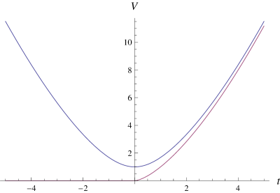
Figure 1: The comparison of classical and quantum behavior of the volume for $w=1/3$, $\alpha=\hbar=a=1$.

IV.3 Energy density and Hubble parameter

First we make use of the unitary mapping $L^{2}(\mathbb{R}_{+},dx)\mapsto L^{2}(\mathbb{R}_{+},dy)$ and map the state $\phi_{a}(x,t)$ accordingly to (33). We find:

$$\phi_{a}(x,t)\mapsto\psi_{a}(y,t):=y^{-1/4}\phi_{a}(2\sqrt{y},t)=\frac{Ny^{1/4}}{(2(a+it))^{3/2}}~{}e^{-\frac{y}{(a+it)}}.$$ (47)

We assume that the action of $\hat{H}$ and $\hat{\rho}$ on $\psi(y)\in L^{2}(\mathbb{R}_{+},dy)$ preserves the Dirichlet condition (i.e. we set $\hat{\rho}=\hat{\rho}_{\infty}$). We perform the Fourier sine transform $FT^{\infty}$ on $\psi_{a}(y,t)$:

$$\tilde{\psi}_{a}(k,t)=\int_{0}^{\infty}\sin(kx)\psi_{a}(x,t)dk=\tilde{N}\frac{\sin(\frac{5}{4}\arctan((a+it)k))}{(\frac{1}{(a+it)^{2}}+k^{2})^{5/8}},$$ (48)

where $\tilde{N}=\frac{N\sqrt{\pi}\Gamma(\frac{5}{4})}{2(a+it)^{3/2}}$ and hence we have

$$\overline{\tilde{\psi}}_{a}\tilde{\psi}_{a}=|\tilde{N}|^{2}\bigg{|}\frac{\sin(\frac{5}{4}\arctan(\frac{k}{C}))}{(C^{2}+k^{2})^{\frac{5}{8}}}\bigg{|}^{2},$$ (49)

where $C=\frac{1}{(a+it)}$. Now, in the momentum representation, the operators $\hat{H}$ and $\hat{\rho}$ are proportional to $k$ and $k^{2}$, respectively. Since the function (49) for large $k$ behaves like

$$\overline{\tilde{\psi}}_{a}\tilde{\psi}_{a}\sim k^{-5/2},$$ (50)

only the operators $\hat{O}$ such that $\hat{O}\leq Ck^{\alpha}$ for large $k$, a constant $C$ and $\alpha<\frac{3}{4}$, are well defined on the states that we consider in the sense that:

$$\langle\hat{O}{\tilde{\psi}}_{a}|\hat{O}\tilde{\psi}_{a}\rangle<\infty.$$ (51)

However, we can still consider the expectation values

$$\langle\tilde{\psi}_{a}|\hat{O}\tilde{\psi}_{a}\rangle:=\langle\hat{O}^{\frac{1}{2}}\tilde{\psi}_{a}|\hat{O}^{\frac{1}{2}}\tilde{\psi}_{a}\rangle,$$ (52)

for operators $\hat{O}\leq Ck^{2\alpha}$. The reason is that the integral $\langle\tilde{\psi}_{a}|k^{2\alpha}\tilde{\psi}_{a}\rangle$ is convergent and since the states $\tilde{\psi}_{a}$ may be approximated by states from the domain of the operator $k^{2\alpha}$ up to arbitrary accuracy, the integral (52) keeps the physical meaning of the expectation value of this operator.

In particular, we may obtain the integral formula for the expectation value of the Hubble parameter (but not the energy density):

$$\langle\tilde{\psi}_{a}|k\tilde{\psi}_{a}\rangle=|\tilde{N}|^{2}\int_{0}^{\infty}\bigg{|}\frac{\sin(\frac{5}{4}\arctan(\frac{k}{C}))}{(C^{2}+k^{2})^{\frac{5}{8}}}\bigg{|}^{2}k~{}dk<\infty.$$ (53)

We have already learnt from the study of the volume that the bounce occurs for the states $\tilde{\psi}_{a}$ at $t=0$, hence we may calculate the expectation value of the operator $\hat{H}=\frac{4}{3w+3}\frac{\hbar}{\alpha}k$ at the bounce:

$$H_{crit}=\frac{\hbar}{\alpha}\cdot\frac{4|\tilde{N}|^{2}}{3w+3}a^{\frac{1}{2}}\int_{0}^{\infty}\bigg{|}\frac{\sin(\frac{5}{4}\arctan(k))}{(1+k^{2})^{\frac{5}{8}}}\bigg{|}^{2}k~{}dk=\frac{\hbar}{\alpha}\cdot\frac{8\Gamma^{2}(\frac{5}{4})\sqrt{2\pi}}{(3w+3)}\cdot\frac{5}{3}\cdot\frac{1}{a}.$$ (54)

After plugging the value of $a$ from (45) into (54), we have:

$$H_{crit}=\frac{16\Gamma^{2}(\frac{5}{4})\sqrt{2\pi}}{(3w+3)}\cdot\frac{5}{3}\cdot\frac{1}{\big{(}\frac{2}{\sqrt{\pi}}\Gamma\big{(}\frac{5+3w}{2+2w}\big{)}\big{)}^{w+1}}\frac{E_{tot}}{\hbar}.$$ (55)

One immediately sees that the value of Hubble parameter at which the universe ‘reverses’ is proportional to the total energy of this universe. Therefore, the more massive the universe, the higher the value of $H_{crit}$. Moreover, one may safely assume that the energy density at the bounce $\rho_{crit}$ is proportional to the square of the total energy $\sim E_{tot}^{2}$.

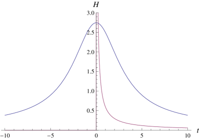
Figure 2: The comparison of classical and quantum behavior of the Hubble parameter for $w=1/3$, $\alpha=\hbar=a=1$. Just after the Big Bounce the quantum universe is shown to expand faster than the classical one, $\langle\hat{H}\rangle>H$. Thus, the quantum universe seems to undergo a kind of inflationary phase.

V Discussion

It is a very interesting conjecture to think that our phase space with the physical quantities like the Hubble parameter and the Hamiltonian is in one to one correspondence with the reduced phase space arising from the identification of Dirac’s observables in the full canonical gauge-symmetry formulation (for a short comment see appendix A). If so, then our Hamiltonian corresponds to a true Hamiltonian in the reduced phase space formulation. This conjecture is investigated in class and a special attention is given to the freedom in fixing an evolution parameter.

Our analysis shows a way to resolve the singularities of classical theory. It started with a Lagrangian that was free from gauge symmetries. The evolution parameter $t$ was treated as a real, absolute time in which the system evolves. This cosmological clock does not exist outside the universe and should be connected with some measurements or change that we observe on cosmological scales. Nevertheless, no matter which quantization method one uses for a gauge system with a Hamiltonian itself being a constraint, one needs an evolution parameter. We argue that the choice of the evolution parameter in such a way that the singularity occurs at its finite value is crucial. Thus a popular free scalar field is not a good choice and we encourage the reader to go through appendix B to see this.

In our approach we managed to express the dynamics of the FRW universe in terms of a freely-moving non-relativistic particle on half-line. The classical dynamics ends when the particle hits the boundary of half-line and the evolution parameter (i.e. the cosmological time) cannot be extended beyond this moment. However, we can promote the Hamiltonian to a self-adjoint operator in quantum theory. Due to the Stone theorem, the self-adjoint Hamiltonian can be exponentiated to a unitary operator, which gives the evolution of the system for the unbounded values of the evolution parameter. Thus, the half-line of the cosmological time is extended to the whole real domain and the singularity is resolved.

We have studied the evolution of quantum states $\phi_{a}$, where $a\in\mathbb{R}_{+}$. How much of the Hilbert space is covered by $\overline{\textrm{Span}}\{\phi_{a}\}$? We study this question and others concerning the evolution of unbounded operators $\hat{\rho}$ and $\hat{H}$ in quant .

We observe in the evolution of the Hubble parameter and the volume of the universe no fixed scale, and in particular Planck scale is irrelevant. The critical values $v_{crit}$ and $H_{crit}$ depend on how massive the universe is in the classical phase of its evolution, which corresponds to the value of $a$. However, we can calculate the value of $\langle\rho\rangle\langle v^{1+w}\rangle$ at the bounce:

$$\alpha H^{2}_{crit}v^{1+w}_{crit}=\frac{\hbar^{2}}{\alpha}\sqrt{2\pi}\cdot 5\cdot(w+1)\bigg{(}\frac{2\Gamma\big{(}\frac{5+3w}{2+2w}\big{)}}{\sqrt{\pi}}\bigg{)}^{w+1}\Gamma^{2}\bigg{(}\frac{5}{4}\bigg{)},$$ (56)

which is clearly independent of the parameter $a$, i.e. of a particular quantum state. Although this quantity is energy dimensionally it is not the same with the energy of the system. Notice that the mean value of energy of the system obtained in (39) depends on a state via the value of $a$. Thus, (56) may signal the existence of some fundamental energy scale not connected with any particular universe. The existence of such scale may enable to fix the value $\alpha$.

This brings us to the problem of determining the value of $\alpha$. First, notice that the choice of $\alpha$ is connected with the choice of time and to this extent it is arbitrary. One may suspect that the study of the conjectured correspondence (appendix A) may shed light on this issues and thus we postpone the investigation to class .

Another indeterminacy of the system is connected with the fact the addition of a total derivative to the Lagrangian in (2) leads to the same dynamics. More importantly, there is an infinite number of ways in which one may define the self-adjoint Hamiltonian. We have restricted to a single choice, preserving the Dirichlet condition. But other choices seem to be equally good and are studied in quant .

Appendix A Relation between reduced phase space equipped with $\mathbb{H}_{true}$ and reduced Lagrangian $\mathbb{L}_{true}$

Suppose one has constructed the reduced phase space equipped with the induced Poisson bracket and a true Hamiltonian $\mathbb{H}_{true}$. In principle, one may now construct an action integral, that is an integral of the Lagrangian $\mathbb{L}_{true}$ defined as a function of the Dirac observables:

$$\mathbb{L}_{true}=P^{J^{\prime}}\dot{{O}}_{J^{\prime}}-\mathbb{H}_{true},$$ (57)

where $P^{J^{\prime}}$ denote the canonical conjugates to ${O}_{J^{\prime}}$ (notice that the number of the Dirac observables is always even) and $\dot{{O}}_{J^{\prime}}=\{{O}_{J^{\prime}},\mathbb{H}_{true}\}_{ind}$.

Therefore, one may begin with a reduced form of Lagrangian $\mathbb{L}_{true}$, which encodes the dynamics of the system in a gauge fixed in correspondence with $\mathbb{H}_{true}$. This formulation should also enjoy a freedom in choice of evolution parameter, hence there should be a class of $\mathbb{L}_{true}$ and a corresponding class of $\mathbb{H}_{true}$.

Appendix B Massless scalar field case

The metric of FRW universe reads:

$$ds^{2}=-N^{2}(\tau)d\tau^{2}+a(\tau)^{2}d\overline{x}^{2},$$ (58)

where $\tau$ is an evolution parameter. The choice of the shift function $N$ corresponds to the choice of the evolution parameter. The rest of the notation as well as the meaning of the variable $l$ used below were explained in section II.

B.1 Lagrangian formulation

For the flat FRW universe with massless scalar field the action reads (see e.g. wald ):

$$S=\frac{3}{16\pi G}\int\frac{{\dot{l}}^{2}l}{N}~{}dt-\frac{1}{2}\int\frac{l^{3}{\dot{\phi}}^{2}}{N}~{}dt,$$ (59)

which leads to the Euler-Lagrange equations:

$$\frac{\delta S}{\delta l}=0 \Rightarrow \frac{3}{16\pi G}\frac{d}{dt}\bigg{(}\frac{2l\dot{l}}{N}\bigg{)}-\frac{3}{16\pi G}\frac{\dot{l}^{2}}{N}+\frac{3}{2}\frac{l^{2}\dot{\phi}^{2}}{N}=0,$$

$$\frac{\delta S}{\delta\phi}=0 \Rightarrow \frac{d}{dt}\bigg{(}\frac{l^{3}\dot{\phi}}{N}\bigg{)}=0,$$

$$\frac{\delta S}{\delta N}=0 \Rightarrow -\frac{1}{N^{2}}\bigg{(}-\frac{3}{16\pi G}\dot{l}^{2}l+\frac{1}{2}l^{3}\dot{\phi}^{2}\bigg{)}=0,$$

to which the solutions in the cosmological time ($N=1$) read:

$$l=\sqrt[3]{\big{(}8\pi G\Omega_{1}\big{)}(t+t_{0})},~{}~{}~{}~{}\phi=\frac{1}{\sqrt{24\pi G}}\ln(t+t_{0})+\frac{3\Omega_{2}}{\sqrt{24\pi G}}.$$ (60)

B.2 Canonical formulation

The Legendre transformation followed by Dirac’s analysis gives:

$$\mathbb{H}=N\bigg{(}\frac{4\pi G}{3}\frac{p_{l}^{2}}{l}-\frac{1}{2}\frac{p_{\phi}^{2}}{l^{3}}\bigg{)},$$ (61)

where the phase space is 4D: $(l,p_{l},\phi,p_{\phi})$, where $p_{l}=\frac{3}{8\pi G}\frac{l\dot{l}}{N}$, $p_{\phi}=-\frac{l^{3}\dot{\phi}}{N}$. The Hamiltonian $\mathbb{H}\approx 0$ is a constraint and $N$ is a non-zero coefficient corresponding to the choice of gauge. Let us look for the Dirac observables via fixing the gauge $N=l^{3}$ and solving:

$$\{O_{i},\mathbb{H}\}=0\Leftrightarrow\bigg{[}\frac{8\pi G}{3}lp_{l}\bigg{(}p_{l}\frac{\partial}{\partial p_{l}}-l\frac{\partial}{\partial l}\bigg{)}+p_{\phi}\frac{\partial}{\partial\phi}\bigg{]}O_{i}=0.$$ (62)

We introduce the new ’geometrical’ variables $X_{\pm}=\ln p_{l}\pm\ln l$ so that the equation (62) reads now:

$$\bigg{[}\frac{16\pi G}{3}e^{X_{+}}\frac{\partial}{\partial X_{-}}+p_{\phi}\frac{\partial}{\partial\phi}\bigg{]}O_{i}=0,$$ (63)

and the solutions are easily found to be:

$$O_{1}=X_{+},~{}~{}~{}~{}O_{2}=p_{\phi},~{}~{}~{}~{}O_{3}=\frac{1}{2}X_{-}-\frac{8\pi G}{3}\frac{e^{X_{+}}}{p_{\phi}}\phi,$$ (64)

which are not independent on the constraint surface due to the identity $\mathbb{H}=\frac{4\pi G}{3}e^{2O_{1}}-\frac{1}{2}O_{2}^{2}$ and for which the Poisson bracket is now modified as follows $dl\wedge dp_{l}=\frac{1}{2}e^{X_{+}}dX_{+}\wedge dX_{-}$. So the complete set of independent elementary Dirac observables consists of two elements, say $O_{1}$ and $O_{3}$, satisfying the algebra:

$$\{O_{1},O_{3}\}=e^{-O_{1}}.$$ (65)

We redefine $\Omega_{1}=e^{O_{1}}$ and $\Omega_{2}=O_{3}-\frac{1}{3}\ln\frac{\sqrt{\Omega_{1}}}{8\pi G}$, so that

$$\{\Omega_{1},\Omega_{2}\}=1,$$ (66)

and we restrict the analysis to the ‘expanding universe’ solutions $\Omega_{1}=lp_{l}>0$ and on the constraint surface we have $O_{3}=\frac{1}{2}X_{-}+\sqrt{\frac{8\pi G}{3}}\phi$. From (60) we have that:

$$l_{\phi}=\sqrt[3]{8\pi G\Omega_{1}e^{-3\Omega_{2}}}e^{\sqrt{\frac{8\pi G}{3}}\phi}.$$ (67)

This quantity is now the Dirac observable for a fixed value of $\phi$, since it does not depend on the value of $t$ that one ascribes to the moment of measurement. The evolution of length is defined as the flow through the parameter $\phi$, which parameterizes the family of Dirac’s observables $l_{\phi}$.

B.3 Classical evolution

Let us identify the generator of the change in $\phi$:

$$\{l_{\phi},\mathbb{H}_{\phi}\}=\partial_{\phi}l_{\phi}\Leftrightarrow\frac{1}{3\Omega_{1}}\frac{\partial\mathbb{H}_{\phi}}{\partial\Omega_{2}}+\frac{\partial\mathbb{H}_{\phi}}{\partial\Omega_{1}}=\sqrt{\frac{8\pi G}{3}}\Leftrightarrow\mathbb{H}_{\phi}=\sqrt{\frac{8\pi G}{3}}\Omega_{1}+f(\frac{1}{3}\ln\Omega_{1}-\Omega_{2}),$$ (68)

where $f$ is arbitrary. How to get rid of this indeterminacy? Note that to parameterize the reduced phase space one needs two independent Dirac’s observables. The first choice was $l_{\phi}$ and what is to be the second? Let us obtain from (60) the Hubble parameter:

$$H_{\phi}=\frac{1}{3}e^{3\Omega_{2}}e^{-3\sqrt{\frac{8\pi G}{3}}\phi},$$ (69)

so that

$$\{H_{\phi},\mathbb{H}_{\phi}\}=\partial_{\phi}H_{\phi}\Leftrightarrow\frac{\partial\mathbb{H}_{\phi}}{\partial\Omega_{1}}=\sqrt{\frac{8\pi G}{3}}\Leftrightarrow\mathbb{H}_{\phi}=\sqrt{\frac{8\pi G}{3}}\Omega_{1}+g(\Omega_{2}),$$ (70)

where $g$ is arbitrary. Now, comparing (68) and (70), removes the indeterminacy and the true Hamiltonian is $\mathbb{H}_{\phi}:=\sqrt{\frac{8\pi G}{3}}\Omega_{1}$. Thus, instead of considering the whole family of $l_{\phi}$ and $H_{\phi}$, which of course produce redundancy in parameterizing the reduced phase space, one fixes the value of $\phi$ and includes the $\mathbb{H}_{\phi}$ as a dynamics generator. One only needs to include that:

$$\{H_{\phi},l_{\phi}\}=-\frac{8\pi G}{3}l_{\phi}^{-2},~{}~{}\{l_{\phi},\mathbb{H}_{\phi}\}=\sqrt{\frac{8\pi G}{3}}l_{\phi},~{}~{}\{H_{\phi},\mathbb{H}_{\phi}\}=-3\sqrt{\frac{8\pi G}{3}}H_{\phi},$$ (71)

where $\mathbb{H}_{\phi}=\sqrt{\frac{3}{8\pi G}}H_{\phi}l_{\phi}^{3}$. Now, let us identify $p_{\phi}$, the conjugate of $l_{\phi}$:

$$\{l_{\phi},p_{\phi}\}=1\Leftrightarrow p_{\phi}=(8\pi G)^{-\frac{1}{3}}e^{-\sqrt{\frac{8\pi G}{3}}\phi}\Omega_{1}^{\frac{2}{3}}e^{\Omega_{2}}+f(\Omega_{1}e^{-3\Omega_{2}})=\frac{3}{8\pi G}l_{\phi}^{2}H_{\phi}+f(l_{\phi}),$$ (72)

where $f$ is arbitrary but we put $f\equiv 0$.

B.4 Quantum evolution

Now, let us collect the information on the system in the form convenient for quantization:

$$\{l,p_{\phi}\}=1,~{}~{}~{}~{}\mathbb{H}=\sqrt{\frac{8\pi G}{3}}lp_{\phi},~{}~{}~{}~{}H=\frac{8\pi G}{3}\frac{p_{\phi}}{l^{2}},~{}~{}~{}~{}\rho=\frac{8\pi G}{3}\frac{p_{\phi}^{2}}{l^{4}},~{}~{}~{}~{}v=l^{3},$$ (73)

where $l>0$, we have dropped the index ${\phi}$ for convenience and thus $l$, $\mathbb{H}$, $H$ and $\rho$ are the length, the Hamiltonian, the Hubble parameter and the energy density, respectively.

We do the following canonical transformation:

$$l\mapsto x=\frac{1}{3}l^{3},~{}~{}~{}~{}p_{\phi}\mapsto p=\frac{p_{\phi}}{l^{2}},$$ (74)

where the new canonical pair $\{x,p\}=1$ is also defined on $\mathbb{R}_{+}\times\mathbb{R}$ and

$$\mathbb{H}=\sqrt{24\pi G}xp,~{}~{}~{}~{}H=\frac{8\pi G}{3}p,~{}~{}~{}~{}\rho=\frac{8\pi G}{3}p,~{}~{}~{}~{}v=3x.$$ (75)

Now, the Schrödinger quantization, $p\mapsto\hat{p}=:-i\frac{d}{dx}$ and $x\mapsto\hat{x}=x$, renders the following formally self-adjoint operators:

$$\hat{\mathbb{H}}=\sqrt{6\pi G}\bigg{(}-ix\frac{d}{dx}-i\frac{d}{dx}x\bigg{)},~{}\hat{H}=\frac{8\pi G}{3}\bigg{(}-i\frac{d}{dx}\bigg{)},~{}\hat{\rho}=\frac{3}{8\pi G}\hat{H}^{2},~{}\hat{v}=3x.$$ (76)

Let us consider the following unitary mapping:

$$R_{+}\ni x,~{}~{}\Psi(x)\mapsto\Phi(y)=\sqrt{2}e^{y}\Psi(e^{2y}),~{}~{}y\in R,$$ (77)

and we find that the Hamiltonian operator in this new Hilbert space reads:

$$\hat{\mathbb{H}}=\sqrt{6\pi G}\big{(}-i\frac{d}{dy}\big{)}.$$ (78)

Now we should ensure that the Hamiltonian is a positive operator, but we will ignore it for it will not alter the fate of the singularity. Now, we can obtain the evolution of wave-functions:

$$e^{i\mathbb{H}\phi}\Phi(y)=\Phi(y+\phi\sqrt{6\pi G})=\sqrt{2}e^{y}e^{\phi\sqrt{6\pi G}}\Psi(e^{2y}e^{2\phi\sqrt{6\pi G}}),$$ (79)

hence the inverse mapping back to the start Hilbert space gives:

$$\sqrt{2}e^{y}e^{\phi\sqrt{6\pi G}}\Psi(e^{2y}e^{2\phi\sqrt{6\pi G}})\mapsto e^{\phi\sqrt{6\pi G}}\Psi(e^{2\phi\sqrt{6\pi G}}x).$$ (80)

Now, we are ready to study the evolution of the expectation value of $\hat{\rho}$:

$$\langle e^{i\mathbb{H}\phi}\Psi(x)|\hat{\rho}~{}e^{i\mathbb{H}\phi}\Psi(x)\rangle=\frac{8\pi G}{3}e^{2\sqrt{24\pi G}\phi}\int\overline{\Psi}(x)-\frac{d^{2}}{dx^{2}}\Psi(x)~{}dx,$$ (81)

and the expectation value of $\hat{v}$:

$$\langle e^{i\mathbb{H}\phi}\Psi(x)|\hat{v}~{}e^{i\mathbb{H}\phi}\Psi(x)\rangle=3e^{-\sqrt{24\pi G}\phi}\int\overline{\Psi}(x)x\Psi(x)~{}dx.$$ (82)

The classical behavior is reproduced in the quantum theory, which includes the unbounded growth of energy density and the vanishing size of the universe.

One may think that this shows that the singularity cannot be resolved in the above system. In fact, however, the singularity problem was not addressed at all due to the peculiar choice of the evolution parameter $\phi$. In order to study the structure of the singularity one has to ensure that the classical singularity occurs at finite value of an evolution parameter.

References

• (1) P. Dirac, ”Lectures on quantum mechanics”, Courier Dover Publications (2001); M. Henneaux, C. Teitelboim, ”Quantization of Gauge Systems”, Princeton University Press (1994).
• (2) P. Malkiewicz and W. Piechocki, “Energy Scale of the Big Bounce,” Phys. Rev.  D 80, 063506 (2009); P. Dzierzak, P. Malkiewicz and W. Piechocki, “Turning big bang into big bounce. 1. Classical dynamics,” Phys. Rev.  D 80, 104001 (2009); P. Malkiewicz, W. Piechocki, ”Turning big bang into big bounce: II. Quantum dynamics”, Class. Quant. Grav. (2010), in press, arXiv:0908.4029.
• (3) J. Derezinski, Lecture Notes “Operators on $L^{2}(\mathbb{R}^{d})$”, http://www.fuw.edu.pl/ derezins/
• (4) P. Malkiewicz, “Problem of time in the reduced phase space of cosmological system”, in preparation.
• (5) P. Malkiewicz, “Quantum Bounce in FRW universe via reduced Lagrangian formulation”, in preparation.
• (6) Robert M. Wald, “General Realtivity”, The University of Chicago Press (1984).