On the transition between the Weibel and the whistler instabilities

Abstract

The transition between non resonant (Weibel-type) and resonant (whistler) instabilities is investigated numerically in plasma configurations with an ambient magnetic field of increasing amplitudes. The Vlasov-Maxwell system is solved in a configuration where the fields have three components but depend only on one coordinate and on time. The nonlinear evolution of these instabilities is shown to lead to the excitation of electromagnetic and electrostatic modes at the first few harmonics of the plasma frequency and, in the case of a large ambient magnetic field, to a long-wavelength, spatial modulation of the amplitude of the magnetic field generated by the whistler instability.

I Introduction

Electron distribution functions that are anisotropic in phase space are a common feature of collisionless plasmas both in space and in the laboratory and the investigation of the processes through which these distributions relax is of primary interest. In fact, the free energy that is made available by the unbalance of the particle “temperatures” in the different directions can be transferred, depending on the plasma conditions, to quasistatic magnetic fields, to electromagnetic or electrostatic coherent structures or to particle acceleration.

The anisotropy of the electron distribution function in an unmagnetized plasma can give rise to the onset of the well known Weibel instabilityWeibel which generates a quasistatic magnetic field.

If a magnetic field is already present in the plasma, the Weibel instability driven by the anisotropy of the electron energy distribution turns into the so called whistler instabilityWIn in which case circularly polarized whistler waves are generated by the relaxation of the electron distribution function. Whistler waves are actually ubiquitous in plasmas and their generation has been extensively studied in recent years in the laboratory (see e.g. Ref.stenzel, ). Whistler instabilities have been reported in spaceWsp where bursts of whistler mode magnetic noise are found to be present in the magnetosphere, close to the magnetopause and are also a likely source of several different magnetospheric fluctuations including plasmaspheric hiss and magnetospheric chorus. These waves propagate along the ambient magnetic field in the frequency range of $\omega_{ci}\leq\omega_{r}\leq\omega_{ce}$, where $\omega_{ce}$ and $\omega_{ci}$ are the electron and proton cyclotron frequencies. A sufficiently large temperature anisotropy in a magnetized plasma is the most commonly observed mechanism for the generation of whistler waves, but additional mechanisms, such as trapped particle loss cone distributions, can also generate these modes.

The linear dispersion relations of these instabilities and how the Weibel instability merges into the whistler instability have been studied in the literatureWW . It has been shownWW that “Weibel-type” whistler modes occur in plasma conditions where the following independent inequalities are satisfied

$$\omega_{r}\leq\gamma\,,\qquad({v_{the,\perp}}/{c})^{2}>({\omega_{ce}}/{\omega_{pe}})^{2},$$ (1)

where $\omega_{r}$ and $\gamma$ are the real and imaginary parts on the mode frequency respectively, and depend on the parallel (${v_{the,||}}$) and on the perpendicular (${v_{the,\perp}}$) thermal velocities of the electrons, and $\omega_{pe}$ is the electron Langmuir frequency. On the contrary, if the above threshold, which we rewrite as

$$\omega_{ce}>\omega_{pe}\sqrt{(A+1)}{v_{the,||}}/{c},$$ (2)

is passed, the growth rates of the whistler instability depart considerably from those of the Weibel instability. In this case the mode frequency $\omega_{r}$ becomes comparable or greater than its growth rate $\gamma$. Here the anisotropy parameter $A$ is defined by $A\equiv(v_{the,\perp}/v_{the,||})^{2}-1$.

In the present paper we consider the long term collisionless relaxation process of an anisotropic electron distribution focusing our attention on the nonlinear features of the transitional regime between the Weibel and the whistler instabilities and on the onset of secondary modes driven by the perturbations in the electron distribution function arising from the nonlinear development of the primary Weibel and whistler instabilities.

The analysis presented here is performed by solving numerically the collisionless Vlasov equation for electrons and protons coupled to Maxwell’s equations, in a restricted geometrical configuration (1D-3V) where all vector quantities are three dimensional but depend on one coordinate only, which is chosen to be the $x$ coordinate, and on time $t$. More specifically, we consider a homogeneous initial plasma configuration with isotropic protons and a bi-Maxwellian electron distribution with $T_{\perp}>T_{||}$ (where “parallel” refers to the $x$ direction) in the presence of a uniform ambient magnetic field $B_{x}$. The ratio between the proton temperature $T_{i}$ and the parallel electron temperature $T_{||}$ is taken equal to one. Vector quantities must be taken to be three dimensional because whistler waves are circularly polarised in the $y$-$z$ plane and in addition we need to include longitudinal electric fields and velocities along $x$. This contrasts the treatment given for the Weibel instability (with ambient magnetic field $B_{x}=0$) given in Ref.lopa1, where a 1D-2V configuration was considered.

At low ambient magnetic field, the nonlinear development of the whistler instability is similar to that of the Weibel instability, since the perturbed magnetic fluctuations are much larger than the ambient magnetic field. However, when the ambient magnetic field is sufficiently strong, the long term nonlinear behaviour of the instability changes drastically. In both limits the isotropization of the electron distribution function due to the onset of the instabilities is accompanied by the development of high frequency (Langmuir wave) electron density modulationslopa1 . These density modulations are forced by the spatial modulation of the magnetic energy density at wave numbers roughly two times the wave numbers of the most unstable Fourier components of the primary instabilities. However these density modulations become weaker as the ambient magnetic field is increased. In addition a purely kinetic effect is present in the small $B_{0}$ limit where the development of the Weibel instability leads to strong deformations of the electron distribution function in phase space. These deformations have been shown in a 1D-2V configurationlopa1 to arise from the differential rotation in velocity space of the electrons around the magnetic field $B_{z}$ produced by the Weibel instability and to generate short wavelength Langmuir modes that form highly localized electrostatic structures corresponding to jumps of the electrostatic potential. These kinetic effects become weaker and eventually disappear as the ambient magnetic field is increased.
In the case of the whistler instability, low-frequency density modulations involving the proton dynamics occur and generate soliton type structures known as whistler oscillitonsSauer . Oscillitons are coherent nonlinear structures that occur in dispersive media for which the curves of the phase and group velocities cross for a finite value of the oscillation wavenumber $k$, see Ref.Sydora, . Whistler oscillitons are of special importance as they have been invoked in order to describe coherent wave emission in the whistler frequency range observed in the Earth’s plasma environmentSauer ; Sydora .

II Numerical set up

In the numerical solutions of the Vlasov-Maxwell system presented below, all the parameters are normalized as follows. We use the plasma frequency $\omega_{pe}$ and the velocity of light $c$ as characteristic frequency and velocity; therefore the electron skin depth $c/\omega_{pe}$ is the characteristic length scale. The electric and magnetic field are normalized to ${\bar{E}}={\bar{B}}=m_{e}c\omega_{pe}/e$ and, finally, the electron temperature is normalized to $m_{e}c^{2}$.

The initial electron anisotropy is kept fixed, $T_{y}=T_{z}=T_{\perp}$,   $T_{||}=T_{x}$,   $T_{\perp}/T_{||}=12$, while the value of $B_{x}$ is varied such that the corresponding electron cyclotron frequency, normalized on the electron Langmuir frequency and indicated in the following simply by $B_{0}$, changes from $B_{0}=0$ to $B_{0}=0.5$. In these numerical integrations Ref.Mangeney, the ratio $\beta_{||}\equiv v_{the,||}^{2}/B_{0}^{2}$ plays the role of a control parameter. Here the parallel thermal velocity $v_{the,||}$ is normalized to $c$ and is chosen to be equal to $0.02$. The following values of $B_{0}$ are chosen, $B_{0}=0,\,0.02,\,0.1,\,$ and $0.5$, corresponding to $\beta_{||}=\infty,\,1,\,4\times 10^{-2},\,$ and $1.6\times 10^{-3}$ respectively.

The number of grid points in coordinate space is $N_{x}=1024$ and the length of the system is $L_{x}=10\pi$ in units of the electron skin depth $d_{e}\equiv c/\omega_{pe}$. The total number of grid points in velocity space is $N_{v_{x}}=101,N_{v_{y}}=N_{v_{z}}=71$. The system is evolved up to the time $t=1200\,\omega_{pe}^{-1}$ with time step $10^{-3}\leq dt\leq 10^{-2}$. The total number of perturbed modes at $t=0$ is $N=220$. The spatial grid spacing is $dx=0.03$. Henceforth $k_{max}\lambda_{D}\ll 1$ and $k_{max}d_{e}\sim 1$, where $k_{max}$ is the the most unstable wave number and $\lambda_{D}$ is the electron Debye length computed with the temperature $T_{||}$. The numerical integrations are initiated in a homogeneous plasma configuration with isotropic protons and Maxwellian electrons with different parallel and perpendicular temperatures by imposing a low amplitude magnetic field noise, randomly oriented in the $y$-$z$ plane at different $x$ positions:

$$B_{y}(x,t=0)=\sum^{N}_{n=1}a_{in}\ [\cos(k_{n}x+\psi_{n})],\qquad B_{z}(x,t=0)=\sum^{N}_{n=1}b_{in}\ [\cos(k_{n}x+\phi_{n})],$$ (3)

with $a_{in}$ and $b_{in}$ the initial ”small” ($\sim 10^{-4}$) amplitudes, $\psi_{n}$ and $\phi_{n}$ random phases, $n$ the wave number and $\mathbf{k}_{n}=2\pi n/L_{x}$ the corresponding wave vector.

In Table 1 we list the main parameters of the numerical runs, together with the analytical (kinetic) value, $\gamma_{max}^{Ana}$ of the growth rate of the most unstable mode, $k=k_{max}$, as obtained, after some simplifications, from Ref.WW, , the corresponding value, $\gamma_{max}^{Num}$, as obtained by the numerical integration of the Vlasov-Maxwell system and the value of the ratio ${\hat{B}}_{z}$ between the amplitudes of the $z$ component of the magnetic field produced by the instability at saturation and that of the ambient magnetic field along $x$.

Instability	${\bf{B_{o}}}$	$\omega_{pe}/\omega_{ce}$	$k_{max}$	$\gamma_{max}^{Ana}$	$\gamma_{max}^{Num}$	${\hat{B}}_{z}$	$\beta_{\|}$	$\beta_{\perp}$
Weibel	0.0	-	1.0	0.034	0.037	-	-	-
Whistler	0.02	50	1.2	0.037	0.038	2.25	1	11.75
	0.10	10	1.2	0.031	0.035	0.56	0.04	0.50
	0.50	2	2.0	0.025	0.020	0.06	0.0016	0.02

Table 1: Main parameters of the numerical runs, the corresponding numerical and analytical growth rates for the most unstable mode corresponding to $k=k_{max}$ and the normalized amplitude at saturation of the $z$ component of the magnetic field produced by the instability.

In Table 2 the real part of the frequency of the whistler unstable mode is shown for different values of $k$ in the “large” ambient magnetic field case $B_{0}=0.5$. For each $k$ three values of the real part of the frequency are shown. Two are analytical: $\omega_{r}^{Ana}(kinetic)$ is obtained, after some simplifications, from Ref.WW, where a kinetic approach is used, and $\omega_{r}^{Ana}(fluid)$ is obtained from Ref.VAL, where a fluid approach is used, while $\omega_{r}^{Num}$ is obtained by numerical integration of the Vlasov-Maxwell system.  The comparison between the analytical and the numerical frequencies and growth rates shows good agreement. The numerical values of the frequencies and growth rates shown in Tables 1-2 are obtained by considering only the linear part of the numerical integration. It should be noted that the comparison for the real frequencies is shown only for ${\bf B}_{0}=0.5$. For the other values of $B_{0}$ in Table 1, the oscillation period would turn out to be longer than the total duration time of the linear regime and it is thus difficult to estimate numerically.

$k$	$\omega_{r}^{Ana}(kinetic)$	$\omega_{r}^{Num}$	$\omega_{r}^{Ana}(fluid)$
0.2	0.02	0.02	0.02
0.4	0.08	0.08	0.08
0.6	0.18	0.13	0.13
0.8	0.32	0.22	0.20
1.0	0.37	0.25	0.25
1.6	0.43	0.40	0.36
2.0	0.45	0.42	0.40
2.4	0.46	0.42	0.42
3.0	0.47	0.45	0.45

Table 2: Mode frequency as a function of $k$ for $B_{0}=0.5$ - Numerical and analytical values.

In Table 3 the real part of the frequency of the most unstable whistler mode, as derived analytically in Ref.VAL, is shown for different values of the ambient magnetic field.

Instability	$B_{0}$	$k_{max}$	$\omega_{r}^{Ana.}$
whistler	0.02	1.20	0.02
	0.10	1.20	0.08
	0.50	2.00	0.47

Table 3: Frequency of the most unstable whistler mode for different ambient magnetic fields

III Whistler modes: transition from weak to strong ambient magnetic field

From Table 1 we see that the growth rate of the whistler instability decreases as the amplitude of the ambient magnetic field increases, while the mode number $k_{max}$, at which the maximum growth rate of the whistler instability is obtained, increases.

By referring to the inequalities (1) we see that for small ambient magnetic field amplitudes both inequalities are satisfied so that the mode frequency and its growth rate are approximately those obtained in Ref.lopa1, for the Weibel instability (zero ambient magnetic field). On the contrary, as the ambient magnetic field amplitude is increased, the system goes through the threshold condition (2) and at the same time the frequency of the whistler waves becomes comparable to, or larger than, their growth rate ($\omega_{r}>\gamma_{max}$). Hence these numerical runs describe the transition regime between Weibel-like, low ambient magnetic field, instabilities and strong ambient magnetic field whistler instabilities.

III.1 Electromagnetic fields

The frequency spectrum of the $z$ component of the perturbed magnetic field is shown in Fig.1 for ${B_{0}=0,\,0.02\,,0.1,\,0.5}$. For each value of the ambient magnetic field $B_{0}$ the most unstable spatial Fourier mode (corresponding to $k=k_{max}$ in Table 1) is chosen. The frequency spectrum is obtained by integrating over time over the whole simulation time ($t=1200\,\omega_{pe}^{-1}$).

Figure 1: Frequency spectrum of the magnetic field component $B_{z,k}$ for $B_{0}=0,0.02,0.1,0.5$ at the corresponding most unstable mode $k=k_{max}=1.0,1.2,1.2,2.0$. Note the change in the amplitude scale in the different frames.

We see a strong peak at $\omega_{r}=0.45$ in the spectrum of the magnetic field with $B_{0}=0.5$ (bottom right frame) which corresponds to the frequency of the whistler wave for $k=k_{max}=2$. This wave is observed at frequencies $\omega_{r}=0.015$ and $\omega_{r}=0.07$ for $B_{0}=0.02$ and for $B_{0}=0.1$, respectively. The whistler peak gets sharper, the stronger the ambient magnetic field. This reduction of the mode ”line width” is consistent with the decrease of the mode growth rate at larger ambient magnetic field values. For comparison, the spectrum for the case $B_{0}=0$ (Weibel case) is also shown: no peak is observed as expected since in an unmagnetized plasma the instability is purely growing.

Figure 2: Frequency spectrum of the electrostatic field component $E_{x,k}$ for $B_{0}=0,0.02,0.1,0.5$ at the corresponding most unstable mode $k=k_{max}=1.6,2.4,2.8,3.6$. Note the change in the amplitude scale in the different frames.

We observe that both in the Weibel and in the whistler cases the frequency spectrum contains waves that propagate with a frequency equal to the plasma frequency, $\omega_{pe}=1$ in the dimensionless units used. In the two intermediate cases, $B_{0}=0.02$ and $B_{0}=0.1$ we also see waves at $2\omega_{pe}$.

Figure 3: Frequency spectrum of the Fourier component of the magnetic field, $B_{z,k}$ for $B_{0}=0.1$ at $k=1.4,4.0,5.0$. Note the change in amplitude scale.

Wave emission with characteristic frequency close to twice the electron plasma frequency are observed near the Earth’s bow shockGurnett1975 and also from type II and III solar radio burstsGoldman . Different mechanisms for the generation of such kind of wave emissions have been discussed in the literature, see Ref.Malaspina, and references therein. Based on the frequency spectrum of the longitudinal electric field $E_{x}$ shown in Fig.2, a plausible mechanism for the $2\omega_{pe}$ emission in our system can be the coupling between forward and backward propagating Langmuir waves that generate an electrostatic mode at $2\omega_{pe}$ which is then converted into an electromagnetic wave by a nonlinear mode coupling process. The amplitude of the $2\omega_{pe}$ component of the perturbed magnetic field is much smaller than that of the waves radiated at the plasma frequency. This small amplitude electromagnetic emission at frequencies close to the harmonics of the plasma frequency is not limited to the modes at $k=k_{max}$ shown in Fig.1 and extends over a range of different values of $k$. Within this range emission at $3\omega_{pe}$ is also observed (Fig.3) at short wavelengths.

Figure 4: Frequency spectrum of the Fourier component of the electrostatic field, $E_{x,k}$ at $k=1.4,4.0,5.0$ for $B_{0}=0$ (top frames) and $B_{0}=0.1$ (bottom frames).

Electromagnetic emission at $3\omega_{pe}$ has been reported in type II bursts Kliem1992 and in type III bursts Benz1973 . Various theories have been put forward in order to explain this higher-harmonic emission. The coalescence of a Langmuir wave and a $2\omega_{pe}$ electromagnetic wave was suggested for the $3\omega_{pe}$ emission in Ref.Zlotnik1978, .
Furthermore, electromagnetic waves with a frequency $\omega_{r}\sim k$ can be seen in the spectra in Fig.3 (see also bottom right frame in Fig.1): their frequency does not correspond to harmonics of the plasma frequency and shifts with $k$. The amplitudes of these latter waves are smaller than those of the $\omega_{pe}$ waves, but greater than those of the $2\omega_{pe}$ and $3\omega_{pe}$ emissions. The higher harmonics emission and the waves at $\omega_{r}\sim k$ are present only at higher wave mode numbers.
Multiple harmonic emission up to fifth harmonic in the Earth’s fore-shock environment has been reported (see Ref.Cairns1986, ). In our simulations the relative intensity of the emission decreases rapidly with increasing harmonic number with harmonics greater than three being too faint to be observed. Although in the magnetic field spectrum we do not observe electromagnetic emission at the fifth harmonic, such high harmonics are observed in the electrostatic spectrum as shown in Fig.4. These $\omega_{pe}$ and higher harmonic emissions are suppressed for larger values of the ambient magnetic field. In a typical solar wind configuration the ratio $\omega_{ce}/\omega_{pe}$ is of the orderParks2003 of $\leavevmode\nobreak\ 10^{-2}$. Hence only the choice of ${\bf B}_{0}=0.02$ or $0.1$ represents a fairly typical situation for this kind of emission. This can be clearly seen from Fig.5 where a contour plot of the perturbed magnetic field $B_{z}$ in the $\omega_{r}$-$k$ plane is shown.

III.2 Electrostatic fields

The frequency spectra of the longitudinal field $E_{x,k}$ at $k=1.4,4,5$ are shown in Fig.4 for $B_{0}=0$ and for $B_{0}=0.1$. In both cases the spectra exhibit a clear peak at the electron plasma frequency. This peak for $B_{0}=0$ appears to be less pronounced for larger values of $k$, consistently with what shown in Ref.lopa1, , while for $B_{0}=0.1$ the amplitude at $\omega_{pe}$ remains almost the same even at smaller wavelengths. In addition in both cases we also see peaks appearing at multiple harmonics of the plasma frequency. It should be noted though that for the unmagnetized plasma case only harmonics up to $4\omega_{pe}$ are observed in contrast to harmonics up to $5\omega_{pe}$ that are observed in the case with $B_{0}=0.1$. The amplitudes of the multiple harmonics of $\omega_{pe}$ for $B_{0}=0.1$ are much larger than in the $B_{0}=0$ case.

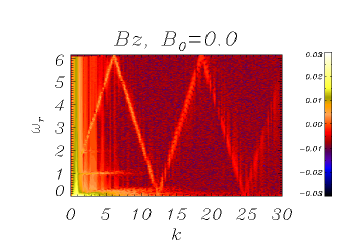
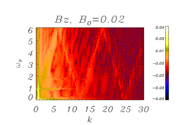
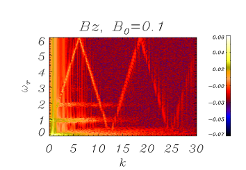
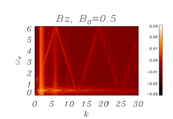
Figure 5: Contour plot of the magnetic field $B_{z}$ in the $\omega_{r}$ - $k$ space for $B_{0}=0,0.02,0.1,0.5$. Note the finite time sampling effect on the frequency electromagnetic waves $\omega_{r}\sim k$ which leads to a “zigzag” pattern. Note the change in the scale of the color coding.

In addition, similarly to the 1D-2V, $B_{0}=0$ analyzed in Ref.lopa1, , electrostatic structures are formed corresponding to plasma modes with values of $k$ larger than those of the whistler waves. For example, for $B_{0}=0$, the resonant velocity corresponding to the clear bump in the distribution function shown in Fig.8 (top right frame) is $v_{r}=0.05$, leading to the excitation of Langmuir waves with wave mode $k\sim\omega_{r}/v_{r}\sim 20$, while for $B_{0}=0.1$, the resonant mode at which the Langmuir waves are excited is $k\sim 10$. As discussed in Ref.lopa1, , these modes are excited by the deformation of the electron distribution function due to the differential rotation of the electrons in phase space in the magnetic field generated in the $y$-$z$ plane by the Weibel and by the whistler instabilities.

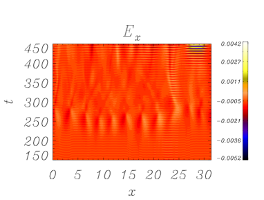
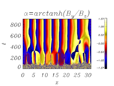
Figure 6: Left frame: contour plot of the electrostatic field in the $x$-$t$ plane (note only a part of the time interval of the total time of the simulation is shown). Right frame: the angle $\alpha=arctanh(B_{y}/B_{z})$ between the magnetic field components in $y$ and $z$ direction in the $x$-$t$ plane.

This deformation becomes weaker as the effect of the ambient magnetic field $B_{0}$ is increased. In addition if we compare the results obtained for $B_{0}=0$ in the 1D-2V case (see Fig.12 in Ref.lopa1, ) with the corresponding results shown in Fig.6 (left frame) for the 1D-3V case, we see that in the latter case the amplitude of these structures is somewhat smaller than in the 2V case. This difference can be attributed to the fact that the 2V case imposes a higher coherency of the perturbed magnetic field which is necessarily oriented along the $z$ axis. On the contrary, in the 3V case considered here, the orientation of the perturbed magnetic field in the $y$-$z$ plane can change as a function of $x$. The eventual formation of coherent electrostatic structures can be attributed to the fact that, for sufficiently long times, the initially randomly orientated perturbed magnetic field becomes fairly organized, as shown by Fig.6 (right frame) where the angle $\alpha=arctanh({B_{y}}/{B_{z}})$ is shown as a function of space and time. This allows for the formation of peaks in the electron distribution function, that are sufficiently coherent in space so as to excite plasma waves by inverse Landau damping, see Figs.7 and 8.

                                 

            

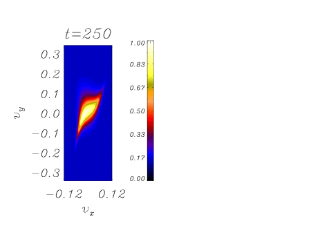
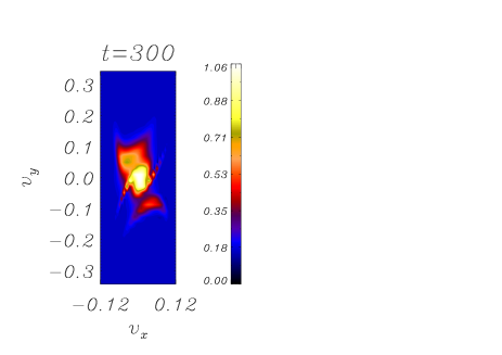
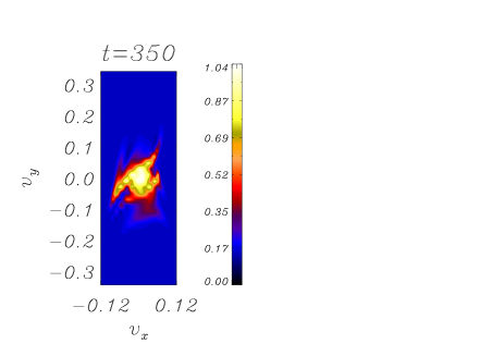
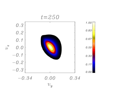
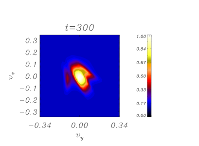
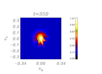
Figure 7: Top frames: Contour plot of the electron distribution function in the $v_{x}$-$v_{y}$ plane (for $v_{z}=0$) for $B_{0}=0$ at $x=1.86$ (position corresponding to the maximum value of the $z$ component of the perturbed magnetic field) for $t=250$, $t=300$, $t=350$. Bottom frames: Contour plot of the distribution function in the $v_{y}$-$v_{z}$ plane (for $v_{x}=0$) at $x=1.86$. Note the different velocity ranges.

The contour plot of the electron distribution function in the $v_{x}$-$v_{y}$ plane for $B_{0}=0$ is shown in Fig.7. The distribution function starts being distorted, with a differential rotation combined with a spreading along $v_{x}$, at the time ($t=300$) when the instability begins to saturate. These deformations become ’multi-armed’ as time evolves. Similar kind of deformations are observed in the $v_{x}$-$v_{z}$ plane (not shown here). Multi-armed structures are also noticeable in the $v_{y}$-$v_{z}$ plane (Fig.7, bottom frames).

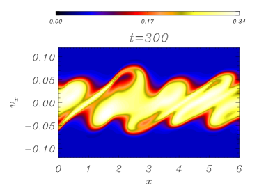
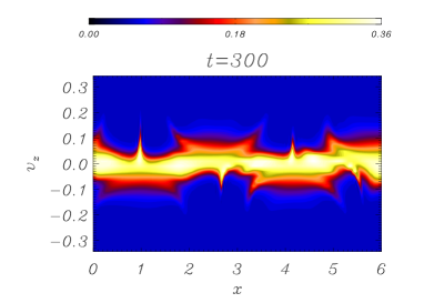
Figure 8: Top frames: The normalized electron distribution function versus $v_{x}$ at $x=1.86$ for $v_{y}=0$ and $v_{z}=0$ for $B_{0}=0$. Bottom (left) frame: Contour plot of the distribution function in the $x$-$v_{x}$ plane at $v_{y}=0$ and $v_{z}=0$ and $x=1.86$. Bottom (right) frame: Contour plot of the distribution function in the $x$-$v_{z}$ plane at $v_{x}=0$ and $v_{y}=0$ and $x=1.86$.

The combined velocity and space dependence of the electron distribution function is shown in Fig.8, bottom frames. The left frame shows the formation of phase space vortices in the $x$-$v_{x}$ plane (shown at $v_{y}=0$ and $v_{z}=0$). The right frame shows alternated filamented structures in the $x$-$v_{z}$ plane. The distribution function for $B_{0}=0.1$ behaves similarly (not shown here), but the strength of the deformations decreases.

III.3 Low frequency modulations

As we have already discussed in Sec.III.2, the distorted distribution function for $B_{0}=0.1$ leads to the resonant excitation of short wavelength plasma waves at large wave numbers, e.g. ($k\sim 10$). On the contrary, at smaller wave numbers we see the interplay between the inhomogeneity of the perturbed magnetic field amplitude and of the electron and proton densities. The electrostatic and the magnetic fields are shown in $x$-$t$ space in Fig.9 for $B_{0}=0.5$. These figures show the forward and the backward propagation of the whistler waves. In addition, long wavelength modulations of the electrostatic structures and of the proton and electron densities are seen in Fig.10 at half the wavelength of the perturbed magnetic field.

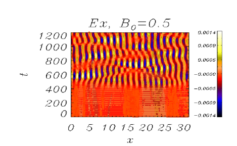
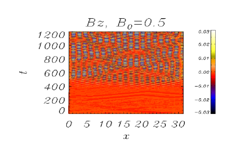
Figure 9: Contour plot of the electrostatic field (left frame) and of the magnetic field (right frame) in the $x$-$t$ plane for $B_{0}=0.5$.

The wavelength of the modulations of both the magnetic field and of the proton and electron densities decreases with increasing ambient magnetic field, the electrostatic field and density modulation wavelength still being equal to half the wavelength of the most unstable Fourier component of the perturbed magnetic field. We focus our attention primarily on the case with ambient magnetic field $B_{0}=0.5$.
There are two kinds of modulations in the perturbed magnetic field, one with long wavelengths having a width almost half the total length of the simulation box, $L\sim 17$ and corresponding time period $T\sim 200$. The phase velocity of these modulations is $v_{ph}\sim 0.08$. The other kind has shorter wavelengths, $L\sim 2$, and $T\sim 7$, i.e. $v_{ph}\sim 0.28$. The range of phase velocities corresponding to the peak in the whistler waves frequency spectrum for different values of $k$ extends from $0.005\leq v_{ph}$ to $v_{ph}\leq 0.25$. Hence, the long wavelength phase velocity $v_{ph}\sim 0.08$, as obtained from the magnetic field modulations, falls in the range of the whistler phase velocities and it can be further noticed that it is comparable with some of the phase velocities obtained for both short wavelength and long wavelength electrostatic modulations which are in the range $0.005\leq v_{ph}\leq 0.01$ and $0.075\leq v_{ph}\leq 0.13$, respectively. Furthermore the range of phase velocities $0.08\leq v_{ph}\leq 0.01$ obtained from low frequency peak, $0.03\leq\omega_{r}\leq 0.04$ in the frequency spectrum of the electrostatic field at the most unstable mode $k_{max}=3.6$ (see Fig.2 bottom right frame) covers a large part of the phase velocity range of the whistler waves.

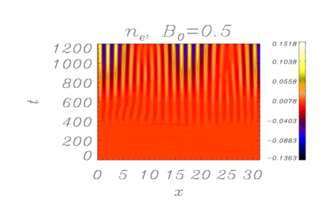
Figure 10: Electron density and proton density for $B_{0}=0.5$.

We can thus infer that the dominant whistler waves are modulated by the low frequency perturbations observed in the electrostatic field. This kind of modulations has been studied theoretically. In Ref.Tripathy, it was proposed that the nonlinear coupling of oppositely travelling waves (forward and backward waves) produce a low frequency ponderomotive force with frequency $\omega=\omega_{1}-\omega_{2}$ and wave vector $k=k_{1}-k_{2}=2k_{1}$. In Refs. Eliasson, and Stenflo, it was later shown that these ponderomotive forces are reinforced due to the interaction of the whistler packets with the background low density perturbations  Eliasson . In addition to the low density perturbations observed in our simulations (see Fig.10), the formation of wave packets of the perturbed magnetic field are also evident (see Fig.11, left frame). Coherent wave emission in the whistler frequency range $(0.1-0.5\omega_{ce})$, consisting of nearly monochromatic wave packets, has recently been observed by several spacecraft in the Earth’s plasma environment Dubinin . These are mainly generated by oscillitons which are stationary, nonlinear structures exhibiting solitary structures with embedded smaller-scale oscillations resembling wave packets. These arise from the momentum exchange between protons and electrons. These oscillitons in the whistler frequency range are known as ’whistler oscillitons’. The appearance of stationary nonlinear waves is related to the existence of a ’resonance point’ where phase and group velocity coincide. The right frame in Fig.11 shows the range of frequencies and wave number available from the numerical results which have a value of their phase velocity close to that of the corresponding group velocity. We also observe a shift of the whistler waves to longer wavelength corresponding to the shift of the broad magnetic spectrum to lower $k$ values during the saturation regime when the coherent whistler emission takes place and modifies the frequency range of the whistler modes.
Observations from laboratory experiments Kostrov exhibit a clear evidence of this kind of modulated whistler wave packets due to nonlinear effects. Furthermore, instruments on board CLUSTER spacecraft have observed Moullard broadband intense electromagnetic waves. Cluster measurements also exhibit the formation of envelop solitary waves accompanied by plasma density cavities. Both electron and proton density cavities formed in our numerical results are shown in Fig.10.

Figure 11: Left frame: Magnetic field versus position at $t=540$. Right frame: The dispersion relation of the whistler waves available which have a value of their phase velocity close to that of the corresponding group velocity.

IV Conclusions

The anisotropy of the electron distribution function ( $T_{\perp}>T_{||}$) has been shown to lead to the onset of both resonant, $\omega_{r}\geq\gamma_{max}$, and non resonant, $\omega_{r}<<\gamma_{max}$, instabilities depending on the value of the ambient magnetic field, see Table 1. When the plasma is unmagnetized the instability (Weibel instability) is completely nonresonant, where $\omega_{r}=0<<\gamma_{max}=0.038$ (in units of the Langmuir frequency), but as we move towards higher ambient magnetic fields, $\omega_{r}$ becomes comparable to the maximum growth rate of the instability. At very high ambient magnetic field ($B_{0}=0.5$, being the value of the electron cyclotron frequency normalized to the Langmuir frequency) the mode becomes resonant with $\omega_{r}$ much larger than the growth rate (whistler instability).
The development of these instabilities is accompanied by the generation of electrostatic and electromagnetic waves at the harmonics of the plasma frequency (up to the fifth harmonic in the case of the electrostatic spectrum).
In addition the spatial self-organization of the perturbed magnetic field leads to the deformation of the electron distribution function and to the consequent generation of short wavelength electrostatic modes. These secondary phenomena tend to be suppressed as the ambient magnetic field becomes larger. On the contrary, at large ambient magnetic field we find a low frequency long wavelength modulation of the whistler wave spectrum that we interpret in terms of the self-consistent interaction between the perturbed magnetic field and the low frequency electron and proton density modulations. The magnetic modulations that we observe are reminiscent of the so called “whistler oscillitons” that arise under the condition that the mode phase velocity coincides with its group velocity.

The simulation results presented here provide relevant information on the different processes that the presence of anisotropy can drive in collisionless plasmas in different plasma magnetization regimes, as parametrized by the value of the parameter $\beta_{\perp}>1$ that gives the ratio between the perpendicular plasma pressure and the ambient magnetic field pressure. For example, in the context of solar physics, the occurrence of resonant whistler modes has been advocated as an effective acceleration mechanisms of electrons directly from the background plasma up to $\sim 25$ MeV within several seconds under normal solar flare conditions Miller .

The simulation results presented in this paper have been obtained by using a 1D configuration and are thus restricted to the study of the nonlinear effects on the system only of modes with parallel wavenumber ${\bf k}$. This restriction will be lifted in a future paper. However, linear analysis Gary2000 indicates that in the presence of low ambient magnetic fields the whistler instability remains the fastest growing one even in a two dimensional configuration where we allow modes to propagate at an angle with respect to the ambient field. On the contrary, at higher ambient magnetic fields where the whistler instability is suppressed, obliquely propagating modes have a larger growth rate. An important question to address in this latter case is how the formation of electrostatic structures will develop in such a regime.

References

References

- (1) Weibel E. 1959 Spontaneously growing transverse waves in a plasma due to an anisotropic velocity distribution, Phys. Rev. Lett. 2 83.
- (2) Gary S. P. et. al. 2006 Linear theory of electron temperature anisotropy instabilities: Whistler, mirror, and Weibel, J. Geophys. Res. 111 A11224.
- (3) Stenzel R. L., Urrutia J. M., and Strohmaier K. D. 2007 Whistler Instability in an Electron-Magnetohydrodynamic Spheromak, Phys. Rev. Lett. 99 265005, and reference therein.
- (4) Contel O. Le et. al. 2009 Quasi-parallel whistler mode waves observed by THEMIS during near-earth depolarization, Ann. Geophysicae 27 2259.
- (5) Lazar M. et. al. 2009 On the existence of Weibel instability in a magnetized plasma. Parallel wave propagation, Phys. of Plasmas 16 012106.
- (6) Palodhi L. et al. 2009 Nonlinear kinetic development of the Weibel instability and the generation of the electrostatic coherent structures, Plasma Phys. and Control. Fusion 51 125006.
- (7) Sauer K. et al. 2002 Wave emission by whistler oscillitons: Application to “coherent lion roars”, Geophys. Res. Lett. 29 2226.
- (8) Sydora R. D. et al. 2007 Coherent whistler waves and oscilliton formation: Kinetic simulations, Geophys. Res. Lett 34 L22105.
- (9) Mangeney, A., Califano F., et al. 2002, A Numerical Scheme for the Integration of the Vlasov-Maxwell System of Equations, Journal of Computational Physics 179 495.
- (10) Valentini F. et al. 2007 A hybrid-Vlasov model based on the current advance method for the simulation of collisionless magnetized plasma, Journal of Computational Physics 225 753
- (11) Gurnett D. A. et al. 1976 Electron plasma oscillations associated with a type III radio bursts, Science 194 1159 .
- (12) Goldman M. V. 1983 Progress and problems in the theory of type III solar radio emission Sol Phys. 89 403.
- (13) Malaspina D. M. et al. 2010 radiation from localized Langmuir waves, J. Geophys. Res. 115 A01101.
- (14) Kliem B. et al. 1992 Third plasma harmonic radiation in type II bursts Sol Phys. 140 149.
- (15) Benz A. O. 1973 Solar radio bursts-Structure of type V event Nat. Phys. Sci. 242 38.
- (16) Zlotanik E. Ya. 1978 Intensity ratio of second and third harmonics in type III solar radio bursts Sov. Astron. 22 228.
- (17) Cairns I. H. 1986 New waves at multiples of the plasma frequency upstream of the earth’s bow shock, J Geophys. Res. 91 2975.
- (18) Park G. 2003 in Physics of space plasma, 2nd ed. Westview Press
- (19) Tripathy V. K. et al. 1988 On the possibility of beat excitation of whistler sidebands in the magnetosphere via ponderomotive force, Geophys. Res. Lett. 15 1299.
- (20) Eliasson et al. 2004 Theoretical and numerical studies of density modulated whistlers, Geophys. Res. Lett. 31 L17802.
- (21) Stenflo L. et al. 1986 Excitation of electrostatic fluctuations by thermal modulation of whistlers J. Geophys. Res. 91 11369.
- (22) Stenzel R. L. 1976 Filamentation of large amplitude whistler waves, Geophys. Res. Lett. 3 61.
- (23) Kostrov et al. 2003 Parametric transformation of the amplitude and frequency of a whistler wave in a magnetoactive plasma, JETP Lett. 78 538.
- (24) Moullard O. et al. 2002 Density modulated whistler mode emissions observed near the plasmapause, Geophys. Res. Lett. 29 36.
- (25) Dubinin E. M. et al. 2007 Coherent whistler emissions in the magnetosphere - cluster observations, Ann. Geophys. 25 303.
- (26) Miller J. A. and Ramaty R. 1987 Ion and relativistic electron acceleration by Alfvèn and whistler turbulence in solar flares, Solar Phys. 113 195.
- (27) Gary S. P. et. al. 2000 Electron temperature anisotropy instabilities: Computer simulations, J. Geophys. Res. 105 10751.