The non-birefringent limit of all linear, skewonless media and its unique light-cone structure

Abstract

Based on a recent work by Schuller et al., a geometric representation of all skewonless, non-birefringent linear media is obtained. The derived constitutive law is based on a “core”, encoding the optical metric up to a constant. All further corrections are provided by two (anti-)selfdual bivectors, and an “axion”. The bivectors are found to vanish if the optical metric has signature (3,1) – that is, if the Fresnel equation is hyperbolic. We propose applications of this result in the context of transformation optics and premetric electrodynamics.

I Introduction

In recent years there has been an increasing effort towards understanding and developing non-birefringent, exotic media. The motivation behind this trend appears to be twofold; on the one hand, many modern metamaterials – particularly in the context of transformation optics Pendry et al. (2006); Leonhardt and Philbin (2006) – are (bi-)anisotropic and yet strictly non-birefringent. On the other hand, the derivation of non-birefringent constitutive relations is a cutting-edge topic in the premetric electrodynamics of spacetime Hehl and Obukhov (2003); Lämmerzahl and Hehl (2004); Itin (2005).

Correspondingly, this paper finds its first application in the design of artificial media whose optical response is independent of the field polarization. Most notably, we derive a simple, relativistic constitutive law which parametrizes all non-birefringent, skewonless materials in terms of a symmetric matrix, two (anti-)selfdual bivectors and an axion. Conveniently, the pivotal symmetric matrix is proportional to the optical metric, while the (anti-)selfdual bivectors vanish if the Fresnel equation is hyperbolic – that is, Lorentzian (3,1). By virtue of this result we also investigate on which transformation media can be attained whilst avoiding birefringence. Remarkably, it emerges that the key choice is to select vacuum as the space on to which to perform the ray-guiding coordinate change. Other options are recognized to be viable. However, they require introducing an axion and/or a metric signature different from $(3,1)$.

A second application of this paper targets the empty space structure of electrodynamics, rather than exotic materials. The seminal works on this topic – due to Hehl, Obukhov and Rubilar Hehl and Obukhov (2003, 2006); Rubilar (2002) – demonstrated that the light-cone structure of spacetime can be re-derived using some minimal, premetric, experimentally justified assumptions. In particular, one obtains the conventional vacuum response merely by setting the skewon part to zero, while enforcing a specific closure condition. A similar, yet separate, scheme is pursued by Lämmerzahl, Hehl Lämmerzahl and Hehl (2004) and Itin Itin (2005). They achieve the customary light-cone by ruling out birefringence and requiring that running-wave solutions must exist in all directions. So far, no link has been made between this latter approach and the former skewonless, closure-abiding one. Our work presents a direct connection, at least for media with no skewon.

This paper is organized as follows: firstly we introduce bi-anisotropic local linear materials, the Fresnel equation and the appropriate relativistic toolbox (Section II). Subsequently, a classification of all non-birefringent media is obtained and the corresponding compact representation is promptly developed (Sections III.1–III.3, and the worked example of Section III.4). The results are then applied both in the context of premetric electrodynamics (Section IV.1) and in the context of transformation optics (Section IV.2). We draw our conclusions in Section V. The Appendices A–C summarize some technical aspects, mostly concerning the work of Ref. Schuller et al. (2010).

II Fresnel equation and non-birefringence of linear media

Since this paper is partly targeted to applications in engineering, we assume the existence of a “background” metric $\overline{\overline{g}}$, thus confining all premetric refinements to Section IV.1. We consider linear, non-dissipative media, for which we introduce a relativistic (frame independent) representation. Suitable starting points are the canonical Boys-Post relations

$$\bm{D} =\overline{\overline{\varepsilon}}\cdot\bm{E}+\overline{\overline{\alpha}}\cdot\bm{B}\ , \bm{H} =\overline{\overline{\beta}}\cdot\bm{E}+\overline{\overline{\mu}}{}^{-1}\cdot\bm{B}\ ,$$ (1)

which define the permittivity $\overline{\overline{\varepsilon}}$, the inverse permeability $\overline{\overline{\mu}}{}^{-1}$ and the magneto-electric couplings $\overline{\overline{\alpha}}$ and $\overline{\overline{\beta}}$ Lindell (2004). More compactly, one can also encode the medium response as:

$$\begin{bmatrix}\bm{D}\\ \bm{H}\end{bmatrix}=\begin{bmatrix}-\overline{\overline{\varepsilon}}&\overline{\overline{\alpha}}\\ -\overline{\overline{\beta}}&\overline{\overline{\mu}}{}^{-1}\end{bmatrix}\begin{bmatrix}-\bm{E}\\ \bm{B}\end{bmatrix}\ .$$ (2)

The 6$\times$6 block matrix, which is identified here, is often labeled $\chi^{IJ}$ – with $I$ and $J$ varying between 1 and 6. Furthermore, it is common practice to introduce the identifications $(F_{I})=(-\bm{E};\bm{B})$ and $(W^{I})=(\bm{D};\bm{H})$. This allows one to re-express the map (2) as:

$$W^{I}=\chi^{IJ}F_{J}\ .$$ (3)

A relativistic notation is now within reach and is achieved by implementing spacetime indices, ranging from 0 to 3 and commonly denoted by Greek letters. With this notation in mind, Eq. (3) is immediately translated to

$$W^{\mu\nu}=\frac{1}{2}\chi^{\mu\nu\alpha\beta}F_{\alpha\beta}\ ,$$ (4)

where the quantities $F_{\alpha\beta}$ and $W^{\alpha\beta}$ are each defined through an appropriate tableau Post (1997):

$$F_{\alpha\beta} =\begin{bmatrix}0&-E_{1}&-E_{2}&-E_{3}\\ E_{1}&0&B_{3}&-B_{2}\\ E_{2}&-B_{3}&0&B_{1}\\ E_{3}&B_{2}&-B_{1}&0\end{bmatrix}\ ,$$ (5)

$$W^{\alpha\beta} =\begin{bmatrix}0&D_{1}&D_{2}&D_{3}\\ -D_{1}&0&H_{3}&-H_{2}\\ -D_{2}&-H_{3}&0&H_{1}\\ -D_{3}&H_{2}&-H_{1}&0\end{bmatrix}\ .$$ (6)

By inspection – or by observing that $F_{\alpha\beta}$ and $W^{\alpha\beta}$ are antisymmetric – one can conclude that each tableau contains only 6 independent entries. These can in turn be collected according to the rule

$$\{[01],[02],[03],[23],[31],[12]\}\rightarrow\{I=1,2,\dots,6\}\ ,$$ (7)

so as to retrieve the 6-dimensional vectors $F_{I}$ and $W^{I}$. Using an analogous argument, since

$$\chi^{\mu\nu\alpha\beta}=-\chi^{\nu\mu\alpha\beta}=-\chi^{\mu\nu\beta\alpha},$$ (8)

one can always switch between the spacetime form $\chi^{\mu\nu\alpha\beta}$ and the 6$\times$6 form $\overline{\overline{\chi}}=\{\chi^{IJ}\}$ . As one might expect, the relativistic representation is particularly convenient when considering a change of frame. More specifically, given an arbitrary non-singular transformation matrix $L^{\alpha^{\prime}}_{\ \alpha}$, one has that (cf. Sec. IV.1)

$$\chi^{\mu^{\prime}\nu^{\prime}\alpha^{\prime}\beta^{\prime}}=L^{\mu^{\prime}}_{\ \mu}L^{\nu^{\prime}}_{\ \nu}L^{\alpha^{\prime}}_{\ \alpha}L^{\beta^{\prime}}_{\ \beta}\,\chi^{\mu\nu\alpha\beta}\ ,$$ (9)

and that the tensors $F_{\alpha\beta}$ and $W^{\alpha\beta}$ behave in a similar manner. For many applications, it is also useful to decompose $\overline{\overline{\chi}}$ by means of the matrix identity

$$\overline{\overline{\chi}}=\frac{\overline{\overline{\chi}}+\overline{\overline{\chi}}{}^{\hskip 2.0ptT}}{2}+\frac{\overline{\overline{\chi}}-\overline{\overline{\chi}}{}^{\hskip 2.0ptT}}{2}=\overline{\overline{\chi}}_{\mbox{\tiny Symm.}}+{{}^{(2)}}\overline{\overline{\chi}}\ ,$$ (10)

whereby one can isolate a symmetric contribution $\overline{\overline{\chi}}_{\mbox{\tiny Symm.}}$ and an antisymmetric contribution ${{}^{(2)}}\overline{\overline{\chi}}$ . A further split, reading

$$\overline{\overline{\chi}}_{\mbox{\tiny Symm.}}={{}^{(1)}}\overline{\overline{\chi}}+{{}^{(3)}}\overline{\overline{\chi}}\ ,$$ (11)

can be achieved by requiring that ${{}^{(1)}}\chi^{[\mu\nu\alpha\beta]}$ vanishes, while ${{}^{(3)}}\chi^{[\mu\nu\alpha\beta]}$ does not. By virtue of (10) and (11), one can finally separate the medium response into a “principal” part, a “skewon” part and an “axion” part:

$$\chi^{\mu\nu\alpha\beta}={{}^{(1)}}\chi^{\mu\nu\alpha\beta}+{{}^{(2)}}\chi^{\mu\nu\alpha\beta}+{{}^{(3)}}\chi^{\mu\nu\alpha\beta}\ ,$$ (12)

where ${{}^{(3)}}\chi^{\mu\nu\alpha\beta}=\alpha\epsilon^{\mu\nu\alpha\beta}$, and $\epsilon^{\mu\nu\alpha\beta}$ is the Levi-Civita tensor defined via

$$\epsilon^{\mu\nu\alpha\beta} =g^{\mu\rho}g^{\nu\sigma}g^{\alpha\eta}g^{\beta\theta}\epsilon_{\rho\sigma\eta\theta}\ ,$$ (13)

$$\epsilon_{0123} =[-\det(\overline{\overline{g}})]^{\frac{1}{2}}\ .$$ (14)

A non-zero ${}^{(2)}\overline{\overline{\chi}}$ component is invariably excluded, since it implies that any of the following common symmetries is broken:

$$\overline{\overline{\varepsilon}}=\overline{\overline{\varepsilon}}{}^{\hskip 2.0ptT}\ ,\quad\quad\overline{\overline{\mu}}=\overline{\overline{\mu}}{}^{\hskip 2.0ptT}\ ,\quad\quad\overline{\overline{\alpha}}=-\overline{\overline{\beta}}{}^{\hskip 2.0ptT}.$$ (15)

By contrast, a finite ${}^{(3)}\overline{\overline{\chi}}$ is still quite rare, but has been observed in nature de Lange and Raab (2001); Hehl et al. (2008) – thus overturning a popular dogma (“Post’s constraint”, see Post (1997); Lakhtakia and Weiglhofer (1995)). The axion field also finds a practical application in the perfect electromagnetic conductor (PEMC) proposed in Lindell and Sihvola (2005). Given these considerations, the present paper assumes that all skewon contributions vanish.

The easiest way to specify the properties of a material is via the 36 entries of $\overline{\overline{\chi}}$. However, when a symbolic calculation must be carried out, it is often more convenient to reduce the constitutive relation to an abstract, more compact form. In engineering, this is mostly attained by simplifying $\overline{\overline{\varepsilon}}$, $\overline{\overline{\mu}}$, $\overline{\overline{\alpha}}$ and $\overline{\overline{\beta}}$ separately, according to their individual symmetry properties Serdyukov et al. (2001). This strategy, however, is manifestly not relativistic, as it involves manipulating the four 3$\times$3 sub-matrices of (2) independently. Therefore, at least for the purpose of this work, one must choose a different approach, where $\chi^{\mu\nu\alpha\beta}$ is decomposed in terms of simpler spacetime quantities. For instance, vacuum is characterized by

$$\chi_{0}^{\mu\nu\alpha\beta}=(\mu_{0}/\varepsilon_{0})^{-\frac{1}{2}}\left(g^{\mu\alpha}g^{\nu\beta}-g^{\mu\beta}g^{\nu\alpha}\right)\ ,$$ (16)

where $g^{\alpha\beta}$ is the inverse of the background metric $g_{\alpha\beta}$. Relaxing some restrictions leads to a first class of non-birefringent materials: the Q-media Lindell and Wallén (2004). These are given by

$$\chi_{\mbox{\tiny Q}}^{\mu\nu\alpha\beta}=s_{Q}\left(Q^{\mu\alpha}Q^{\nu\beta}-Q^{\mu\beta}Q^{\nu\alpha}\right)\ ,$$ (17)

with $s_{Q}=\pm 1$, and provide three supplementary sources of flexibility. Firstly, the tensor $Q^{\alpha\beta}$ is not a metric, since although it is invertible, it is not necessarily symmetric. In the context of this paper, this property has little relevance, since a vanishing skewon implies that either $\overline{\overline{Q}}=-\overline{\overline{Q}}{}^{\hskip 2.0ptT}$ or $\overline{\overline{Q}}=\overline{\overline{Q}}{}^{\hskip 2.0ptT}$. Insomuch as the former case leads to an unspecified wave (co-)vector Bergamin (2010), only the latter case can be accepted. Thus, $\overline{\overline{Q}}$ can henceforth be considered to be a “constitutive” metric, converging to $\overline{\overline{g}}$ for the vacuum (16). Accordingly, media of type (17) will be referred to as “metric media”. Secondly, the constitutive signature need not be $(3,1)$, that is, “Lorentzian”. This attribute will prove essential in deriving a compact representation for all non-birefringent materials (Section III). Lastly, the impedance of the medium in Eq. (17) can be calculated to be

$$\sqrt{\frac{|\det({Q}^{-1}_{\alpha\beta})|}{-\det(g_{\alpha\beta})}}\ ,$$ (18)

and is not necessarily equal to $(\mu_{0}/\epsilon_{0})^{\frac{1}{2}}$. Moreover, the sign $s_{Q}$ allows one to obtain a negative index of refraction Bergamin and Favaro (2010).

A further class of materials, which naturally extends Q-media, has been proposed by Wallén and Lindell Lindell (2004); Lindell and Wallén (2004). They modify (17) by including two “bivectors” (antisymmetric tensors) $\bm{A}$ and $\bar{\bm{A}}$:

$$\chi_{\mbox{\tiny genQ}}^{\mu\nu\alpha\beta}=s_{Q}\left(Q^{\mu\alpha}Q^{\nu\beta}-Q^{\mu\beta}Q^{\nu\alpha}\right)+A^{\mu\nu}\bar{A}^{\alpha\beta}\ ,$$ (19)

where, in this article, one must enforce $\bar{\bm{A}}=s_{A}\bm{A}$ with $s_{A}=\pm 1$, since ${}^{(2)}\overline{\overline{\chi}}$ is assumed to vanish.

Formulating the constitutive relation is the first step in characterizing the behaviour of light. The second milestone consists in solving Maxwell’s equations – in general or, as in the present work, in two specific circumstances. When studying the structure of exotic spacetimes, the propagation of sharp electromagnetic fronts is considered Hehl and Obukhov (2003). By contrast, when modeling laboratory materials, some approximate plane-wave analysis is implemented (the light’s front-velocity in a table-top medium is always exactly $c$ Milonni (2002, 2005)). Both of these scenarios correspond to the so-called “geometrical optics” limit, whence a dispersion (“Fresnel”) relation, linking the angular frequency $\omega$ to the spatial frequency $\bm{k}$, is derived. Using frame-independent notation, the 4-wave co-vector $\bm{K}=(-\omega,\bm{k})$ is found to obey

$$\epsilon_{\alpha\beta\gamma\delta}\epsilon_{\eta\theta\kappa\lambda}\chi^{\alpha\beta\eta\theta}\chi^{\gamma\mu\nu\kappa}\chi^{\delta\rho\sigma\lambda}K_{\mu}K_{\nu}K_{\rho}K_{\sigma}=0\,,$$ (20)

that is, a quartic Fresnel polynomial, cubic in the medium parameters Hehl and Obukhov (2003); Rubilar (2002); Obukhov et al. (2000); Lindell (2005); Itin (2009). By using Eq. (12), one can also prove that the effect of the axion on this formula is zero. Consequently, it impossible to specify ${{}^{(3)}}\overline{\overline{\chi}}$ by analyzing light propagation in bulk.

A material is non-birefringent if the Fresnel polynomial becomes bi-quadratic:

$$(G^{\alpha\beta}K_{\alpha}K_{\beta})^{2}=0\ ,$$ (21)

where $\overline{\overline{G}}$ is an “optical” metric. For an explicit derivation of the non-birefringence conditions we refer to the literature Lämmerzahl and Hehl (2004); Itin (2005) (cf. Section III.4). The Fresnel equation for a Q-medium is trivial ($G^{\alpha\beta}\!\propto\!Q^{\alpha\beta}$). However, that of its extension (19) is not Lindell (2004):

$$\!\!\left[Q^{\mu\nu}K_{\mu}K_{\nu}\right]\!\left[\left(\overline{\overline{Q}}-s_{A}\bm{A}\cdot\overline{\overline{Q}}{}^{-1}\cdot\bm{A}\right)^{\alpha\beta}K_{\alpha}K_{\beta}\right]=0\ .$$ (22)

Birefringence, as induced by the bivector $\bm{A}$, can be eliminated by requiring that

$$\bm{A}\cdot\overline{\overline{Q}}{}^{-1}\cdot\bm{A}=a\overline{\overline{Q}}\ ,$$ (23)

where the proportionality constant $a$ may vanish, but $a\neq s_{A}$. The generalized Q-media that satisfy (23) cover only a range of non-birefringent materials. Nonetheless, they provide essential guidance for the generic case.

III Geometric representation of all non-birefringent media

III.1 From Schuller’s classification to a compact form

Discovering specific examples of non-birefringent media is relatively easy. However, finding a general representation is – at a first sight – difficult, given the complicated structure of the Fresnel equation (20) . Remarkably, a classification scheme recently proposed by Schuller et al. Schuller et al. (2010), brings this task to the realm of possibility (at least for a vanishing skewon field). The key breakthrough comes from an in-depth analysis of the Segre types Hall (2004); Stephani et al. (2003) emerging from the modified tensor

$$\kappa_{\mu\nu}{}^{\rho\sigma}=\frac{1}{2}\epsilon_{\mu\nu\alpha\beta}\chi^{\alpha\beta\rho\sigma}\ .$$ (24)

As an outcome, 23 equivalence classes are obtained, each equipped with a normal form (or “typical representative”), whereby a complete categorization is readily achieved – an arbitrary “symmetric” constitutive tensor can be linked uniquely to a typical representative by using a change of frame. Simultaneously, the non-birefringence conditions developed in Lämmerzahl and Hehl (2004); Itin (2005) are invariant under any basis transformation, as dictated by the principle of relativity. Therefore, an observer independent coverage of all non-birefringent media can be fully attained from the 23 specific matrices of Ref. Schuller et al. (2010) – complying, in this sense, with the main aim of this section.

A few technical comments are in order. Schuller et al. opt to classify the lower-indexed “area metric” $G_{\mu\nu\rho\sigma}$, rather than the upper-indexed $\chi^{\mu\nu\rho\sigma}$ which is favored here. Regardless of this choice, the normal forms that they derive do apply directly to $\overline{\overline{\chi}}$. In addition, the representatives in Ref. Schuller et al. (2010) are subject to the condition $\det\overline{\overline{\chi}}=1$. We choose to temporarily suspend this constraint, since the procedures below never preclude us from achieving a unit determinant. As a final remark, one should notice that Schuller et al. employ an alternative 6$\times$6 index ordering – compare equation (2) in Ref. Schuller et al. (2010) with equation (7) of this manuscript.

With the help of computational software, the required non-birefringent classification is derived straightforwardly. The immediate outcome is a set of matrices, which provide a valid solution, but not a transparent answer (see Appendices A and B). In spite of this difficulty, one necessary – but not sufficient – condition does emerge clearly. The structure

$$\chi_{\mbox{\tiny NBR}}^{\mu\nu\rho\sigma}= \,s_{Q}\left(Q^{\mu\rho}Q^{\nu\sigma}-Q^{\mu\sigma}Q^{\nu\rho}\right)$$

$$+ \,s_{A}A^{\mu\nu}A^{\rho\sigma}+s_{\tilde{A}}\tilde{A}^{\mu\nu}\tilde{A}^{\rho\sigma}+\alpha\epsilon^{\mu\nu\rho\sigma}\ ,$$ (25)

encompasses efficiently all skewonless non-birefringent materials, although some polarization-dependent solutions are yet to be ruled out. A complete refinement will soon be obtained. Nonetheless, some essential remarks should not be avoided. Equation (25) is designed to conveniently encode the optical metric, solely by means of $\overline{\overline{Q}}$. Moreover, our compact form naturally generalizes Eq. (19), at the small price of including an innocuous axion offset. It is also important to realize that the representation (25) is invariant under some “bivector space” transformations comprising $\bm{A}$ and $\tilde{\bm{A}}$. If $s_{A}s_{\tilde{A}}=1$, trigonometric rotations of the form

$$\begin{pmatrix}\bm{A}^{\prime}\\ \tilde{\bm{A}}^{\prime}\end{pmatrix}=\begin{pmatrix}\cos\phi&-\sin\phi\\ \sin\phi&\cos\phi\end{pmatrix}\cdot\begin{pmatrix}\bm{A}\\ \tilde{\bm{A}}\end{pmatrix}$$ (26)

map the medium tensor onto itself. If $s_{A}s_{\tilde{A}}=-1$, proper rotations have to be replaced by hyperbolic rotations

$$\begin{pmatrix}\bm{A}^{\prime}\\ \tilde{\bm{A}}^{\prime}\end{pmatrix}=\begin{pmatrix}\cosh\varphi&-\sinh\varphi\\ -\sinh\varphi&\cosh\varphi\end{pmatrix}\cdot\begin{pmatrix}\bm{A}\\ \tilde{\bm{A}}\end{pmatrix}\ .$$ (27)

III.2 Necessary and sufficient conditions imply duality

At this point, the crucial idea is to study the Fresnel equation of $\chi_{\mbox{\tiny NBR}}^{\mu\nu\rho\sigma}$, so as to find a true, minimal, non-birefringent representation. From Eq. (20):

$$\det[\overline{\overline{Q}}]\Bigl{(}(\overline{\overline{Q}}-s_{Q}s_{A}\bm{A}\cdot\overline{\overline{Q}}{}^{-1}\cdot\bm{A})^{\mu\nu}K_{\mu}K_{\nu}\times\\ \times(\overline{\overline{Q}}-s_{Q}s_{\tilde{A}}\tilde{\bm{A}}\cdot\overline{\overline{Q}}{}^{-1}\cdot\tilde{\bm{A}})^{\rho\sigma}K_{\rho}K_{\sigma}\\ -s_{A}s_{\tilde{A}}\left[(\bm{A}\cdot\overline{\overline{Q}}{}^{-1}\cdot\tilde{\bm{A}})^{\mu\nu}K_{\mu}K_{\nu}\right]^{2}\Bigr{)}=0\ .$$ (28)

Thus, the medium is non-birefringent if and only if the following conditions are met:

$$\bm{A}\cdot\overline{\overline{Q}}{}^{-1}\cdot\bm{A}\cdot\overline{\overline{Q}}{}^{-1}=a_{1}\mathds{1}\ ,$$ (29)

$$\tilde{\bm{A}}\cdot\overline{\overline{Q}}{}^{-1}\cdot\tilde{\bm{A}}\cdot\overline{\overline{Q}}{}^{-1}=a_{2}\mathds{1}\ ,$$ (30)

$$\bm{A}\cdot\overline{\overline{Q}}{}^{-1}\cdot\tilde{\bm{A}}\cdot\overline{\overline{Q}}{}^{-1}+\tilde{\bm{A}}\cdot\overline{\overline{Q}}{}^{-1}\cdot\bm{A}\cdot\overline{\overline{Q}}{}^{-1}=2a_{3}\mathds{1}\ .$$ (31)

Here, the scalars $a_{1}$, $a_{2}$ and $a_{3}$ must always comply with:

$$(1-s_{Q}s_{A}a_{1})(1-s_{Q}s_{\tilde{A}}a_{2})-s_{A}s_{\tilde{A}}a_{3}\neq 0\ .$$ (32)

A solution to the above constraints is easily found by exploiting the bivector identity

$$\frac{1}{2}A^{\mu\rho}\epsilon^{Q}_{\rho\nu\alpha\beta}A^{\alpha\beta}=\pm\frac{\sqrt{|\det\bm{A}|}}{\sqrt{|\det\overline{\overline{Q}}|}}\delta^{\mu}_{\nu}\ ,$$ (33)

where $\epsilon^{Q}_{\mu\nu\alpha\beta}$ is a Levi-Civita-type tensor, with dual $\epsilon_{Q}^{\mu\nu\alpha\beta}$:

$$\epsilon^{Q}_{0123} =|\det(\overline{\overline{Q}})|^{-\frac{1}{2}}\ ,$$ (34)

$$\epsilon_{Q}^{\mu\nu\alpha\beta}\! =Q^{\mu\rho}Q^{\nu\sigma}Q^{\alpha\eta}Q^{\beta\theta}\epsilon^{Q}_{\rho\sigma\eta\theta}\ ,$$ (35)

$$\Rightarrow\quad\quad\quad(\epsilon_{Q})^{IJ}\! =\mbox{sgn}[\det(\overline{\overline{Q}})](\epsilon_{Q}^{-1})^{IJ}\ .$$ (36)

Applying the relation (33) in Eqs. (29) and (30), yields our main results; namely,

$$A^{\mu\nu} =\frac{s_{X}}{2}\epsilon_{Q}^{\mu\nu\alpha\beta}(\overline{\overline{Q}}{}^{-1}\cdot\bm{A}\cdot\overline{\overline{Q}}{}^{-1})_{\alpha\beta}:=s_{X}({{}^{*}\!\bm{A}})^{\mu\nu}\ ,$$ (37)

$$\tilde{A}^{\mu\nu} =\frac{s_{Y}}{2}\epsilon_{Q}^{\mu\nu\alpha\beta}(\overline{\overline{Q}}{}^{-1}\cdot\tilde{\bm{A}}\cdot\overline{\overline{Q}}{}^{-1})_{\alpha\beta}:=s_{Y}({{}^{*}\!\tilde{\bm{A}}})^{\mu\nu}\ ,$$ (38)

that is, $\bm{A}$ and $\tilde{\bm{A}}$ must be selfdual ($s_{X},s_{Y}=1$) or anti-selfdual ($s_{X},s_{Y}=-1$), with:

$$\bm{A} ={{}^{**}}\!\bm{A}\ , \tilde{\bm{A}} ={{}^{**}}\!\tilde{\bm{A}}\ .$$ (39)

The additional condition (31) is solved automatically, provided $s_{X}=s_{Y}$.

Rotating the constraints (29)–(31) by means of Eq. (26), determines that $a_{3}=0$ can be achieved whenever $s_{A}s_{\tilde{A}}=1$. By contrast, if $s_{A}s_{\tilde{A}}=-1$, the hyperbolic rotations (27) allow one to attain $a_{3}=0$ only when

$$\frac{a_{1}+a_{2}}{a_{3}}\notin[-2,+2]\ .$$ (40)

III.3 A summary with all explicit solutions to duality

In summary it is found that the optical metric of any non-birefringent medium obeys $G^{\mu\nu}\!\propto\!Q^{\mu\nu}$. All non-birefringent, skewonless materials are characterized by a Q-medium “core”, which encodes the optical metric. Two (anti-)selfdual bivectors and an axion term can be included as corrections, but they do not affect the dispersion relation. Any further discussion needs to distinguish between the three possible signatures of $\overline{\overline{Q}}$.

III.3.1 Signature (3,1)

When the signature of $\overline{\overline{Q}}$ is Lorentzian (3,1), the following identity is true for any bivector $\bm{\psi}$ Hehl and Obukhov (2003):

$$\bm{\psi}=-{{}^{**}}\bm{\psi}\ .$$ (41)

Correspondingly, equation (39) cannot be satisfied, unless $\bm{A}\equiv 0$ and $\tilde{\bm{A}}\equiv 0$. Then, any non-birefringent material, with hyperbolic Fresnel equation, is simply a metric medium – complemented by an eventual axion. Some observations in this sense can also be found in the group theory analysis of Ref. Schuller et al. (2010).

III.3.2 Signatures (4,0) and (2,2)

The remaining two signatures support finite (anti-) selfdual bivector corrections. These can be written in terms of the vectors $\bm{\tau}$, $\bm{u}$ and $\bm{v}$, such that:

$$A^{\mu\nu} =2\tau^{[\mu}u^{\nu]}+s_{X}\epsilon_{Q}^{\mu\nu\rho\sigma}(\overline{\overline{Q}}{}^{-1}\cdot\bm{\tau})_{\rho}(\overline{\overline{Q}}{}^{-1}\cdot\bm{u})_{\sigma}\ ,$$ (42)

$$\tilde{A}^{\mu\nu} =2\tau^{[\mu}v^{\nu]}+s_{X}\epsilon_{Q}^{\mu\nu\rho\sigma}(\overline{\overline{Q}}{}^{-1}\cdot\bm{\tau})_{\rho}(\overline{\overline{Q}}{}^{-1}\cdot\bm{v})_{\sigma}\ .$$ (43)

In this parametrization, $\bm{\tau}$ singles out a particular direction, according to which all other vectors can be decomposed. In this sense, $\bm{\tau}$ plays a role similar to that of a time vector, and can be selected independently of $\bm{A}$ and $\tilde{\bm{A}}$ – in almost all cases. Complications arise only if the signature is (2,2) and $\bm{\tau}$ is light-like, a scenario that we shall resolve later. Thus, one can take

$$\bm{\tau}\cdot\overline{\overline{Q}}{}^{-1}\cdot\bm{\tau}\neq 0\ ,$$ (44)

while no specific signature is assumed yet. The components of $\bm{u}$ and $\bm{v}$ parallel to $\bm{\tau}$ never contribute to Eqs. (42) and (43). Therefore, given that we excluded a light-like $\bm{\tau}$, one can choose $\bm{\tau}\cdot\overline{\overline{Q}}{}^{-1}\cdot\bm{u}=0$ and $\bm{\tau}\cdot\overline{\overline{Q}}{}^{-1}\cdot\bm{v}=0$, with no loss of generality. With these simplifications, it is possible to derive the following relations:

$$a_{1} =-(\bm{\tau}\cdot\overline{\overline{Q}}{}^{-1}\cdot\bm{\tau})(\bm{u}\cdot\overline{\overline{Q}}{}^{-1}\cdot\bm{u})\ ,$$ (45)

$$a_{2} =-(\bm{\tau}\cdot\overline{\overline{Q}}{}^{-1}\cdot\bm{\tau})(\bm{v}\cdot\overline{\overline{Q}}{}^{-1}\cdot\bm{v})\ ,$$ (46)

$$a_{3} =-(\bm{\tau}\cdot\overline{\overline{Q}}{}^{-1}\cdot\bm{\tau})(\bm{u}\cdot\overline{\overline{Q}}{}^{-1}\cdot\bm{v})\ .$$ (47)

If $\overline{\overline{Q}}$ has signature (4,0), a true norm is established. Thus, the occurrence of $a_{1}=0$ or $a_{2}=0$ is forbidden, unless $\bm{\tau}$, $\bm{u}$ or $\bm{v}$ vanish. By means of trigonometric or hyperbolic rotations, the orthogonality $\bm{u}\cdot\overline{\overline{Q}}{}^{-1}\cdot\bm{v}=0$ can be obtained without altering $\overline{\overline{\chi}}_{\mbox{\tiny NBR}}$. Equivalently, $a_{3}=0$ can always be assumed. Hence, for signature (4,0), the three vectors $\bm{\tau}$, $\bm{u}$ and $\bm{v}$ can be chosen to be mutually Q-orthogonal, with no effect on the medium response.

If $\overline{\overline{Q}}$ has signature (2,2), the situation is more complicated. The vectors $\bm{u}$ and $\bm{v}$ can be light-like, thereby allowing $a_{1}=0$ and $a_{2}=0$. Moreover, if $s_{A}s_{\tilde{A}}=-1$, one can find cases where $a_{3}=0$ is no longer achievable.

Finally, we should comment on the possibility of a light-like $\bm{\tau}$. This choice is more subtle since there exist pairs of vectors $(\bm{\tau},\bm{u})$ obeying all of the following conditions:

$$\tau^{[\mu}u^{\nu]} \neq 0\ , \bm{\tau}\cdot\overline{\overline{Q}}{}^{-1}\cdot\bm{u} =0\ ,$$ (48)

$$\bm{\tau}\cdot\overline{\overline{Q}}{}^{-1}\cdot\bm{\tau} =0\ , \bm{u}\cdot\overline{\overline{Q}}{}^{-1}\cdot\bm{u} =0\ .$$ (49)

Pairs of this kind span the kernel of the map (42), which links two vectors to one bivector. Whilst in specific situations one could allow for a light-like $\bm{\tau}$, this choice is inconvenient in general.

III.4 A worked example: revision and further details

A worked example is proposed, which provides hands-on revision for Sections III.1–III.3. By implementing the prescriptions of Refs. Lämmerzahl and Hehl (2004); Itin (2005), a specific “Schuller” normal form is explicitly reduced to the non-birefringent limit (25). Two bivectors, playing the role of $A^{\alpha\beta}$ and $\tilde{A}^{\alpha\beta}$, are readily determined. Their structure is shown to be encompassed by Eqs. (42) and (43), thus illustrating a specific instance of (anti-)selfduality.

As explained in Section III.1, choosing a typical representative singles out a Segre type. In turn, this identifies a set of eigenvalues for the modified medium tensor of Eq. (24); in this example, we select the characteristics

$$\sigma_{1}+\mbox{i}\tau_{1},\quad\sigma_{1}-\mbox{i}\tau_{1},\quad\lambda_{1},\quad\lambda_{2},\quad\lambda_{3},\quad\lambda_{4},$$ (50)

where $\sigma_{1},\tau_{1},\lambda_{1},\dots,\lambda_{4}$ are real scalars. The associated 6$\times$6 matrix normal form $\chi_{\mbox{\tiny NF}}^{IJ}$ reads

$$\overline{\overline{\chi}}_{\mbox{\tiny NF}}=\left[\begin{array}[]{cccccc}-\tau_{1}&0&0&\sigma_{1}&0&0\\ 0&\lambda_{3}&0&0&\lambda_{4}&0\\ 0&0&\lambda_{1}&0&0&\lambda_{2}\\ \sigma_{1}&0&0&\tau_{1}&0&0\\ 0&\lambda_{4}&0&0&\lambda_{3}&0\\ 0&0&\lambda_{2}&0&0&\lambda_{1}\end{array}\right]\ ,$$ (51)

as reported in Ref. Schuller et al. (2010) (cf. “metaclass VI” therein, with the index ordering (7)). At this point, the optical properties of the material are fully specified and the Fresnel equation (20) can be invoked to obtain the polynomial

$$M_{0}q^{4}+M_{1}q^{3}+M_{2}q^{2}+M_{3}q+M_{4}=0\ ,$$ (52)

where $q$ is a component picked arbitrarily from the wave co-vector $K_{\mu}$. Crucially, the coefficients $M_{0},\dots,M_{4}$ are still a function of $(-\omega,\bm{k})$; however, they are independent of the particular entry $K_{\nu}$ such that $q\!=\!K_{\nu}$. For the material under consideration, if $q$ coincides with $\!K_{1}$:

$$M_{0}= -\lambda_{1}\lambda_{3}\tau_{1}\ ,$$ (53)

$$M_{1}= \ 0\ ,$$ (54)

$$M_{2}= +K_{0}^{2}\tau_{1}\left[-\lambda_{1}^{2}+\left(\lambda_{2}-\lambda_{4}\right){}^{2}-\lambda_{3}^{2}\right]$$

$$-K_{3}^{2}\lambda_{3}\left[-\lambda_{1}^{2}+\left(\lambda_{2}-\sigma_{1}\right){}^{2}+\tau_{1}^{2}\right]$$

$$-K_{2}^{2}\lambda_{1}\left[-\lambda_{3}^{2}+\left(\lambda_{4}-\sigma_{1}\right){}^{2}+\tau_{1}^{2}\right]\ ,$$ (55)

$$M_{3}= -2K_{0}K_{2}K_{3}\ \times$$

$$\big{\{}\! +\lambda_{2}^{2}\left(\lambda_{4}-\sigma_{1}\right)-\lambda_{1}^{2}\left(\lambda_{4}-\sigma_{1}\right)$$

$$-\sigma_{1}\left[\lambda_{3}^{2}-\lambda_{4}\left(\lambda_{4}-\sigma_{1}\right)\right]$$

$$-\lambda_{4}\tau_{1}^{2}+\lambda_{2}\left(\lambda_{3}^{2}-\lambda_{4}^{2}+\sigma_{1}^{2}+\tau_{1}^{2}\right)\!\big{\}}\ ,$$ (56)

$$M_{4}= -K_{0}^{4}\lambda_{1}\lambda_{3}\tau_{1}\ +K_{2}^{4}\lambda_{1}\lambda_{3}\tau_{1}\ +K_{3}^{4}\lambda_{1}\lambda_{3}\tau_{1}$$

$$+K_{2}^{2}K_{3}^{2}\tau_{1}\left[\lambda_{1}^{2}+\lambda_{3}^{2}-\left(\lambda_{2}-\lambda_{4}\right){}^{2}\right]$$

$$-K_{0}^{2}K_{2}^{2}\lambda_{3}\left[\tau_{1}^{2}-\lambda_{1}^{2}+\left(\lambda_{2}-\sigma_{1}\right){}^{2}\right]$$

$$-K_{0}^{2}K_{3}^{2}\lambda_{1}\left[\tau_{1}^{2}-\lambda_{3}^{2}+\left(\lambda_{4}-\sigma_{1}\right){}^{2}\right]\ ,$$ (57)

as one can verify by using a numerical software (see Footnote 9). Two topics ought to be addressed: firstly, the identifications (53)–(57) depend on the choice of $q$, in contrast with the relativistic standard retained so far; secondly, birefringence must still be eliminated through the reduction of Eq. (52) to the form (21).

Remarkably, once a bi-quadratic $(G^{\alpha\beta}K_{\alpha}K_{\beta})^{2}\!=\!0$ is derived, the result is independent of how $q$ is defined. This fact can be verified directly, by means of a computer, or geometrically from the uniqueness of the “light-cone” Lämmerzahl and Hehl (2004). Knowing that (when birefringence is ruled out) a frame independent outcome is ensured, one can safely apply the scheme of Figure 1 and retrieve Eq. (21).

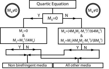
Figure 1: The procedure to make Eq. (52) a bi-quadratic. One must check that $M_{4}\!\neq\!0$ at every node, so as to avoid $q\!=\!0$. The birefringence elimination scheme proposed in Refs. Lämmerzahl and Hehl (2004); Itin (2005) does not include the $M_{0}\!=\!0$ branch depicted on the left.

The analysis underpinning this method is due to Lämmerzahl, Hehl Lämmerzahl and Hehl (2004) and Itin Itin (2005). The present example demonstrates that, in extension to the existing theory, non-birefringent solutions can be obtained even for $M_{0}\!=\!0$ (Fig. 1, left-hand branch). By contrast, $M_{4}$ must always be nonzero, otherwise the dispersion relation (52) leads to the unphysical root $q\!=\!0$. Carrying out the procedure described in Figure 1 for the medium (51) yields

$$M_{0} =0\,, \qquad\lambda_{1} =0\,, \qquad\lambda_{2} =\pm\lambda_{3}+\lambda_{4}\,,$$ (58)

$$M_{0} =0\,, \qquad\lambda_{3} =0\,, \qquad\lambda_{4} =\pm\lambda_{1}+\lambda_{2}\,,$$ (59)

$$M_{0} =0\,, \qquad\tau_{1} =0\,, \qquad\sigma_{1} =\pm\lambda_{3}+\lambda_{4}\,,$$ (60)

$$M_{0} =0\,, \qquad\tau_{1} =0\,, \qquad\sigma_{1} =\pm\lambda_{1}+\lambda_{2}\,,$$ (61)

whilst taking $M_{0}\!\neq\!0$ provides no results compatible with

$$M_{4}\neq\frac{\left(4M_{0}M_{2}-M_{1}^{2}\right)^{2}}{64M_{0}^{3}}\ .$$ (62)

It is worth noticing that the eigenvalues in Eq. (50) can be re-ordered, for example by exchanging $\lambda_{3}$ with $\lambda_{1}$ and $\lambda_{4}$ with $\lambda_{2}$. Accordingly, one can observe that Eqs. (59) and (61) are equivalent to Eqs. (58) and (60), respectively. With no loss of generality, it is thus possible to focus on the two cases

$$\mbox{(i)}\qquad\quad\lambda_{3} =0\,, \ \lambda_{4} =-\zeta\lambda_{1}+\lambda_{2}\,,$$ (63)

$$\mbox{(ii)}\qquad\quad\tau_{1} =0\,, \ \sigma_{1} =+\zeta\lambda_{1}+\lambda_{2}\,,$$ (64)

with $\zeta\!=\!\pm 1$. The corresponding Fresnel equations (20) are non-birefringent, as required, and read

$$-\lambda_{1}[(\lambda_{2}-\sigma_{1}-\zeta\lambda_{1})^{2}+\tau_{1}^{2}](K_{1}K_{2}\!+\!\zeta K_{0}K_{3})^{2}\!= 0,$$ (65)

$$-\lambda_{1}[(\lambda_{2}-\lambda_{4}+\zeta\lambda_{1})^{2}-\lambda_{3}^{2}](K_{1}K_{2}\!+\!\zeta K_{0}K_{3})^{2}\!= 0.$$ (66)

Moreover, the pre-factors multiplying $(K_{1}K_{2}\!+\!\zeta K_{0}K_{3})^{2}$ must be non-zero, otherwise the dispersion relation vanishes identically. One thus enforces the conditions

$$\mbox{(i)}\,\qquad\lambda_{1} \neq 0, (\lambda_{2}-\sigma_{1}-\zeta\lambda_{1})^{2}+\tau_{1}^{2} \neq 0,$$ (67)

$$\mbox{(ii)}\qquad\lambda_{1} \neq 0, (\lambda_{2}-\lambda_{4}+\zeta\lambda_{1})^{2}-\lambda_{3}^{2} \neq 0,$$ (68)

so as to identify the optical metrics for cases (i) and (ii):

$$\overline{\overline{G}}_{\mbox{\tiny(i)}}=\overline{\overline{G}}_{\mbox{\tiny(ii)}}=\left(\begin{array}[]{cccc}0&0&0&1\\ 0&0&\zeta&0\\ 0&\zeta&0&0\\ 1&0&0&0\end{array}\right)\ .$$ (69)

As an aside, one should observe that $\overline{\overline{G}}_{\mbox{\tiny(i)}}$ and $\overline{\overline{G}}_{\mbox{\tiny(ii)}}$ have signature $(2,2)$. Hence, these metrics are not suitable for governing the causal structure of spacetime Schuller et al. (2010); Rätzel et al. (2010). All realizations of Eq. (69) are restricted to laboratory materials, in the steady-state limit (Section II). In agreement with the findings of Section III.1, the non-birefringent media (63) and (64) have a constitutive relation of the form (25). More specifically, one can show that

$$\chi_{\mbox{\tiny(i)}}^{\mu\nu\rho\sigma}= -\mbox{sgn}(\lambda_{1})\left(Q_{\mbox{\tiny(i)}}^{\mu\rho}Q_{\mbox{\tiny(i)}}^{\nu\sigma}-Q_{\mbox{\tiny(i)}}^{\mu\sigma}Q_{\mbox{\tiny(i)}}^{\nu\rho}\right)$$

$$+s_{\mbox{\tiny(i)}}A_{\mbox{\tiny(i)}}^{\mu\nu}A_{\mbox{\tiny(i)}}^{\rho\sigma}\>+\tilde{s}_{\mbox{\tiny(i)}}\tilde{A}_{\mbox{\tiny(i)}}^{\mu\nu}\tilde{A}_{\mbox{\tiny(i)}}^{\rho\sigma}\>+\lambda_{2}\epsilon^{\mu\nu\rho\sigma}\ ,$$ (70)

$$\chi_{\mbox{\tiny(ii)}}^{\mu\nu\rho\sigma}= -\mbox{sgn}(\lambda_{1})\left(Q_{\mbox{\tiny(ii)}}^{\mu\rho}Q_{\mbox{\tiny(ii)}}^{\nu\sigma}-Q_{\mbox{\tiny(ii)}}^{\mu\sigma}Q_{\mbox{\tiny(ii)}}^{\nu\rho}\right)$$

$$+s_{\mbox{\tiny(ii)}}A_{\mbox{\tiny(ii)}}^{\mu\nu}A_{\mbox{\tiny(ii)}}^{\rho\sigma}+\tilde{s}_{\mbox{\tiny(ii)}}\tilde{A}_{\mbox{\tiny(ii)}}^{\mu\nu}\tilde{A}_{\mbox{\tiny(ii)}}^{\rho\sigma}+\lambda_{2}\epsilon^{\mu\nu\rho\sigma}\ ,$$ (71)

where the two constitutive metrics $Q_{\mbox{\tiny(i)}}^{\alpha\beta}$ and $Q_{\mbox{\tiny(ii)}}^{\alpha\beta}$ coincide

$$\overline{\overline{Q}}_{\mbox{\tiny(i)}} =\sqrt{|\lambda_{1}|}\ \overline{\overline{G}}_{\mbox{\tiny(i)}}, \overline{\overline{Q}}_{\mbox{\tiny(ii)}} =\sqrt{|\lambda_{1}|}\ \overline{\overline{G}}_{\mbox{\tiny(ii)}},$$ (72)

and are non-singular by virtue of Eqs. (67) and (68). The bivector corrections $\bm{A}_{\mbox{\tiny(i)}},\tilde{\bm{A}}_{\mbox{\tiny(i)}},\bm{A}_{\mbox{\tiny(ii)}}$ and $\tilde{\bm{A}}_{\mbox{\tiny(ii)}}$ are given by

$$\bm{A}_{\mbox{\tiny(i)}}\!= \!\left[\begin{array}[]{cccc}0&a_{\mbox{\tiny(i)}}&0&0\\ -a_{\mbox{\tiny(i)}}&0&0&0\\ 0&0&0&b_{\mbox{\tiny(i)}}\\ 0&0&-b_{\mbox{\tiny(i)}}&0\end{array}\right]\ ,$$ (77)

$$\tilde{\bm{A}}_{\mbox{\tiny(i)}}\!= \!\left[\begin{array}[]{cccc}0&c_{\mbox{\tiny(i)}}&0&0\\ -c_{\mbox{\tiny(i)}}&0&0&0\\ 0&0&0&d_{\mbox{\tiny(i)}}\\ 0&0&-d_{\mbox{\tiny(i)}}&0\end{array}\right]\ ,$$ (82)

$$\bm{A}_{\mbox{\tiny(ii)}}\!= \!\left[\begin{array}[]{cccc}0&0&a_{\mbox{\tiny(ii)}}&0\\ 0&0&0&b_{\mbox{\tiny(ii)}}\\ -a_{\mbox{\tiny(ii)}}&0&0&0\\ 0&-b_{\mbox{\tiny(ii)}}&0&0\end{array}\right]\ ,$$ (87)

$$\tilde{\bm{A}}_{\mbox{\tiny(ii)}}\!= \!\left[\begin{array}[]{cccc}0&0&c_{\mbox{\tiny(ii)}}&0\\ 0&0&0&d_{\mbox{\tiny(ii)}}\\ -c_{\mbox{\tiny(ii)}}&0&0&0\\ 0&-d_{\mbox{\tiny(ii)}}&0&0\end{array}\right]\ ,$$ (92)

where the real scalars $\{a_{\mbox{\tiny(i)}},\dots,d_{\mbox{\tiny(i)}}\}$ and $\{a_{\mbox{\tiny(ii)}},\dots,d_{\mbox{\tiny(ii)}}\}$ must be expressed in terms of the eigenvalues (50). Similarly, the signs $\{s_{\mbox{\tiny(i)}},\tilde{s}_{\mbox{\tiny(i)}},s_{\mbox{\tiny(ii)}},\tilde{s}_{\mbox{\tiny(ii)}}\}$ are still to be specified. One can directly verify that, defining the variables

$$\rho_{\mbox{\tiny(i)\,}} :=-\zeta\lambda_{1}-\lambda_{2}+\sigma_{1}\ ,$$ (93)

$$\rho_{\mbox{\tiny(ii)}} :=+\zeta\lambda_{1}-\lambda_{2}+\lambda_{4}\ ,$$ (94)

$$\xi_{\mbox{\tiny(ii)}} :=\mbox{sgn}(|\lambda_{3}|\!-\!|\rho_{\mbox{\tiny(ii)}}|)\ ,$$ (95)

and selecting the signs $s_{\mbox{\tiny(i)}},\tilde{s}_{\mbox{\tiny(i)}},s_{\mbox{\tiny(ii)}}$ and $\tilde{s}_{\mbox{\tiny(ii)}}$ according to

$$s_{\mbox{\tiny(i)}\,} =\mbox{sgn}(\tau_{1})\,, \tilde{s}_{\mbox{\tiny(i)}\,} =-\>\>\mbox{sgn}(\tau_{1})\,\,,$$ (96)

$$s_{\mbox{\tiny(ii)}} =\mbox{sgn}(\lambda_{3})\,, \tilde{s}_{\mbox{\tiny(ii)}} =\xi_{\mbox{\tiny(i)}}\mbox{sgn}(\lambda_{3})\,,$$ (97)

is compatible with the following choice of bivector entries:

$$a_{\mbox{\tiny(i)}} =-\,d_{\mbox{\tiny(i)}}\ ,$$ (98)

$$b_{\mbox{\tiny(i)}} =+\,c_{\mbox{\tiny(i)}}\ ,$$ (99)

$$c_{\mbox{\tiny(i)}} =+\,\mbox{sgn}(\tau_{1})\ [(|\rho_{\mbox{\tiny(i)}}|^{2}+|\tau_{1}|^{2})^{\frac{1}{2}}+|\tau_{1}|]^{\frac{1}{2}}/\sqrt{2}\ ,$$ (100)

$$d_{\mbox{\tiny(i)}} =-\,\mbox{sgn}(\rho_{\mbox{\tiny(i)}})[(|\rho_{\mbox{\tiny(i)}}|^{2}+|\tau_{1}|^{2})^{\frac{1}{2}}-|\tau_{1}|]^{\frac{1}{2}}/\sqrt{2}\ ,$$ (101)

$$a_{\mbox{\tiny(ii)}} =+\,\xi_{\mbox{\tiny(ii)}}\,\mbox{sgn}(\lambda_{3})\,\mbox{sgn}(\rho_{\mbox{\tiny(ii)}})\,b_{\mbox{\tiny(ii)}}\ ,$$ (102)

$$c_{\mbox{\tiny(ii)}} =-\,\xi_{\mbox{\tiny(ii)}}\,\mbox{sgn}(\lambda_{3})\,\mbox{sgn}(\rho_{\mbox{\tiny(ii)}})\,d_{\mbox{\tiny(ii)}}\ ,$$ (103)

$$b_{\mbox{\tiny(ii)}} =+\left[|\lambda_{3}|-\xi_{\mbox{\tiny(ii)}}|\rho_{\mbox{\tiny(ii)}}|\right]^{\frac{1}{2}}/\sqrt{2}\ ,$$ (104)

$$d_{\mbox{\tiny(ii)}} =+\left[|\rho_{\mbox{\tiny(ii)}}|+\xi_{\mbox{\tiny(ii)}}|\lambda_{3}|\right]^{\frac{1}{2}}/\sqrt{2}\ .$$ (105)

As a final consistency check, it is possible to verify that the conditions (37) and (38) are satisfied. In fact, one can demonstrate that

$$A^{\mu\nu}_{\mbox{\tiny(i)\phantom{i}}}= 2\tau_{\mbox{\tiny(i)\phantom{i}}}^{[\mu}u_{\mbox{\tiny(i)\phantom{i}}}^{\nu]}+\zeta\epsilon_{Q_{\mbox{\tiny(i)}}}^{\mu\nu\rho\sigma}(\overline{\overline{Q}}{}^{-1}_{\mbox{\tiny(i)}}\cdot\bm{\tau}_{\mbox{\tiny(i)}})_{\rho}(\overline{\overline{Q}}{}^{-1}_{\mbox{\tiny(i)}}\cdot\bm{u}_{\mbox{\tiny(i)}})_{\sigma}\,,$$ (106)

$$\tilde{A}_{\mbox{\tiny(i)\phantom{i}}}^{\mu\nu}= 2\tau_{\mbox{\tiny(i)\phantom{i}}}^{[\mu}v_{\mbox{\tiny(i)\phantom{i}\,}}^{\nu]}+\zeta\epsilon_{Q_{\mbox{\tiny(i)}}}^{\mu\nu\rho\sigma}(\overline{\overline{Q}}{}^{-1}_{\mbox{\tiny(i)}}\cdot\bm{\tau}_{\mbox{\tiny(i)}})_{\rho}(\overline{\overline{Q}}{}^{-1}_{\mbox{\tiny(i)}}\cdot\bm{v}_{\mbox{\tiny(i)}})_{\sigma}\,,$$ (107)

$$A^{\mu\nu}_{\mbox{\tiny(ii)}}= 2\tau_{\mbox{\tiny(ii)}}^{[\mu}u_{\mbox{\tiny(ii)}}^{\nu]}+\zeta\epsilon_{Q_{\mbox{\tiny(ii)}}}^{\mu\nu\rho\sigma}(\overline{\overline{Q}}{}^{-1}_{\mbox{\tiny(ii)}}\cdot\bm{\tau}_{\mbox{\tiny(ii)}})_{\rho}(\overline{\overline{Q}}{}^{-1}_{\mbox{\tiny(ii)}}\cdot\bm{u}_{\mbox{\tiny(ii)}})_{\sigma}\,,$$ (108)

$$\tilde{A}_{\mbox{\tiny(ii)}}^{\mu\nu}= 2\tau_{\mbox{\tiny(ii)}}^{[\mu}v_{\mbox{\tiny(ii)\,}}^{\nu]}+\zeta\epsilon_{Q_{\mbox{\tiny(ii)}}}^{\mu\nu\rho\sigma}(\overline{\overline{Q}}{}^{-1}_{\mbox{\tiny(ii)}}\cdot\bm{\tau}_{\mbox{\tiny(ii)}})_{\rho}(\overline{\overline{Q}}{}^{-1}_{\mbox{\tiny(ii)}}\cdot\bm{v}_{\mbox{\tiny(ii)}})_{\sigma}\,,$$ (109)

where the triplets $\{\bm{\tau}_{\mbox{\tiny(i)}},\bm{u}_{\mbox{\tiny(i)}},\bm{v}_{\mbox{\tiny(i)}}\}$ and $\{\bm{\tau}_{\mbox{\tiny(ii)}},\bm{u}_{\mbox{\tiny(ii)}},\bm{v}_{\mbox{\tiny(ii)}}\}$ are specified (non-uniquely) as

$$\bm{\tau}_{\mbox{\tiny(i)}\phantom{i}}= \ (0,1,0,0)\ ,$$ (110)

$$\bm{u}_{\mbox{\tiny(i)\phantom{i}}}= \ (a_{\mbox{\tiny(i)}}/15,0,0,b_{\mbox{\tiny(i)}}/17)\ ,$$ (111)

$$\bm{v}_{\mbox{\tiny(i)\phantom{i}}}= \ (c_{\mbox{\tiny(i)}}/15,0,0,d_{\mbox{\tiny(i)}}/17)\ ,$$ (112)

$$\bm{\tau}_{\mbox{\tiny(ii)}}= \ (0,0,1,0)\ ,$$ (113)

$$\bm{u}_{\mbox{\tiny(ii)}}= \ (a_{\mbox{\tiny(ii)}}/17,0,0,b_{\mbox{\tiny(ii)}}/15)\ ,$$ (114)

$$\bm{v}_{\mbox{\tiny(ii)}}= \ (c_{\mbox{\tiny(ii)}}/17,0,0,d_{\mbox{\tiny(ii)}}/15)\ .$$ (115)

Clearly, the bivectors (77)–(92) display the typical structure (42)-(43). Thus, the corrections $\bm{A}_{\mbox{\tiny(i)}},\dots,\tilde{\bm{A}}_{\mbox{\tiny(ii)}}$ are selfdual for $\zeta=+1$, and anti-selfdual for $\zeta=-1$.

IV Unique light-cone and transformation optics

IV.1 The light-cone and premetric electrodynamics

This section is organized as follows: firstly, some refinements are introduced, as required by the premetric electrodynamics of spacetime. Then, it is demonstrated that the results of Section III remain valid, besides all amendments. Finally, the work of Ref. Hehl and Obukhov (2003) is linked to that of Ref. Lämmerzahl and Hehl (2004).

Following the premetric formalism of Post Post (1997), the mathematics used so far needs one adjustment. The permutation symbols $e^{\alpha\beta\gamma\delta}$ and $\hat{e}_{\alpha\beta\gamma\delta}$, with

$$e^{0123} =1\ , \hat{e}_{0123} =1\ ,$$ (116)

must be employed. Correspondingly, it is necessary to go beyond the rules of tensor transformation, since

$$e^{\alpha^{\prime}\beta^{\prime}\gamma^{\prime}\delta^{\prime}}=|\det(L^{\rho^{\prime}}_{\ \rho})|^{-1}L^{\alpha^{\prime}}_{\ \alpha}L^{\beta^{\prime}}_{\ \beta}L^{\gamma^{\prime}}_{\ \gamma}L^{\delta^{\prime}}_{\ \delta}\,e^{\alpha\beta\gamma\delta}\ ,$$ (117)

where the “density” factor $|\det(L^{\rho^{\prime}}_{\ \rho})|^{-w}$ is said to have “weight” $w\!=\!+1$. Given that the premetric medium response $\overline{\overline{\chi}}_{\mbox{\tiny PM}}$ is a derived quantity Hehl and Obukhov (2003),

$$\chi_{\mbox{\tiny PM}}^{\mu\nu\alpha\beta}:=\frac{1}{2}e^{\mu\nu\rho\sigma}\kappa_{\rho\sigma}{}^{\alpha\beta}\ ,$$ (118)

the following “amended” transformation rule is obtained (compare with Eq. (9))

$$\chi_{\mbox{\tiny PM}}^{\mu^{\prime}\nu^{\prime}\alpha^{\prime}\beta^{\prime}}=|\det(L^{\rho^{\prime}}_{\ \rho})|^{-1}L^{\mu^{\prime}}_{\ \mu}L^{\nu^{\prime}}_{\ \nu}L^{\alpha^{\prime}}_{\ \alpha}L^{\beta^{\prime}}_{\ \beta}\,\chi_{\mbox{\tiny PM}}^{\mu\nu\alpha\beta}\ ,$$ (119)

so that $\chi_{\mbox{\tiny PM}}^{\mu\nu\alpha\beta}$ is a tensor density with weight $w=+1$.

At this point, we verify that the refinements (117) and (119) do not affect the findings of Section III. Crucially, one can prove (cf. Appendix C) that Schuller’s classification still applies, and that the representation (25) is translated to:

$$\chi_{\mbox{\tiny PM}}^{\mu\nu\rho\sigma}= \sqrt{|\det(Q^{-1}_{\alpha\beta})|}M\bigl{[}\left(Q^{\mu\rho}Q^{\nu\sigma}-Q^{\mu\sigma}Q^{\nu\rho}\right)$$

$$+ \,s_{A}A^{\mu\nu}A^{\rho\sigma}+s_{\tilde{A}}\tilde{A}^{\mu\nu}\tilde{A}^{\rho\sigma}\bigr{]}+\alpha e^{\mu\nu\rho\sigma}\ ,$$ (120)

where $M$ is a true scalar. The “differences” between Eq. (IV.1) and the counterpart (25) drop out from the Fresnel equation. Hence, the expression (28) is always obtained, together with the conditions (37) and (38). Consequently, all the conclusions of Section III remain valid.

To understand the importance of our work in the context of premetric electrodynamics, a few results of this program should be mentioned. Hehl and Obukhov Hehl and Obukhov (2003) consider some key experimental facts, and thus deduce a constitutive metric – a “light-cone” structure – emerging from the response $\overline{\overline{\chi}}_{\mbox{\tiny PM}}$. By enforcing electric-magnetic reciprocity, they require the axion free contribution $\tilde{\chi}^{IJ}_{\mbox{\tiny PM}}$ to obey the closure condition

$$\hat{e}_{IK}\tilde{\chi}_{\mbox{\tiny PM}}^{KL}\hat{e}_{LM}\tilde{\chi}_{\mbox{\tiny PM}}^{MJ}=\tilde{\kappa}_{I}{}^{K}\tilde{\kappa}_{K}{}^{J}=-\left(1/\tilde{Z}^{2}\right)\delta_{I}^{J}\ ,$$ (121)

where $\tilde{Z}$ is a constant. As a second and final constraint, they also set the skewon part to zero, so as to obtain the desired Lorentzian metric – together with an arbitrary axion contribution. In Ref. Lämmerzahl and Hehl (2004) Lämmerzahl and Hehl exploit different observational facts and develop a parallel, yet unrelated, derivation. Rather than simplifying the material response directly, they study the characteristics of the Fresnel equation, thus achieving an optical metric. They impose that:

• The medium is non-birefringent, that is, there exists a factorization of the form (21). Hence, an optical metric is uniquely defined.

• Given a value of $\omega$, the optical metric supports two real (“running-wave”) solutions – accordingly, the Fresnel polynomial is hyperbolic.

Clearly, the two schemes presented above are conceptually distant. Ref. Hehl and Obukhov (2003) proceeds by exploiting symmetries, and deduces a constitutive metric $\overline{\overline{Q}}$. By contrast, Ref. Lämmerzahl and Hehl (2004) takes a strictly “eikonal” route, and derives an optical metric $\overline{\overline{G}}$. Given these differences, it is remarkable that, in the absence of skewon, we can indeed establish a link: as seen in Section III, the optical metric for all non-birefringent media is proportional to the constitutive metric, $Q^{\alpha\beta}\propto G^{\alpha\beta}$. Observing that vacuum must have signature $(3,1)$ , the result $\bm{A}\equiv\tilde{\bm{A}}\equiv 0$ is found immediately. Thus, the distinction between constitutive and optical structures disappears:

$$\!\!\chi_{\mbox{\tiny PM}}^{\mu\nu\rho\sigma}\!=\frac{\tilde{Z}^{-1}}{\sqrt{-\det G^{\alpha\beta}}}\left[G^{\mu\rho}G^{\nu\sigma}\!\!-\!G^{\mu\sigma}G^{\nu\rho}\right]+\alpha e^{\mu\nu\rho\sigma},$$ (122)

up to a choice of $\tilde{Z}$ and $\alpha$. These residual sources of flexibility do not distinguish the works of Ref. Hehl and Obukhov (2003) and Ref. Lämmerzahl and Hehl (2004). Indeed, Hehl and Obukhov “manually” set $\tilde{Z}=(\mu_{0}/\epsilon_{0})^{1/2}$ and $\alpha=0$ in (D.6.11) and (D.6.12).

IV.2 Non-birefringent transformation optics

Transformation optics (TO) is a useful design tool, which offers direct control over the light rays Pendry et al. (2006); Leonhardt and Philbin (2006). Its working principle is simple and can be explained in few sentences. The starting point is always a well-understood setup, called “base-geometry”, supporting a pre-determined electromagnetic configuration. A coordinate change, or “deformation”, is then applied, which drags the fields to a useful layout – and which specifies the necessary medium parameters. Thereby, a powerful recipe is spelled out, which can be used to engineer materials with tailored optical properties. Novel devices can thus be developed in the laboratory, whilst dissolving any reference to the enabling grid-distortion.

Most applications of TO, such as cloaking Pendry et al. (2006); Leonhardt (2006); Li and Pendry (2008), light-harvesting Aubry et al. (2010) and lensing Pendry (2003), make use of a simple base-geometry: usually vacuum, or an arrangement of scalar $\varepsilon$ and $\mu$. By virtue of this choice, birefringence is always ruled out from the very outset and never affects the design process. For many purposes, this is a true benefit, which should be exploited fully; whence the question: what is the most general substrate for constructing a TO scheme free of birefringence?

In the case of zero skewon, a complete answer comes from the analysis of Section III. In particular, any material featured in the base-geometry must take the compact form (25), whilst obeying the duality rules (37) and (38). A number of interesting scenarios are encompassed in this general solution – for example, when the signature is (4,0) or (2,2). Yet it appears that, technologically, the Lorentzian metric does enjoy a special status, since it guarantees propagating bulk modes. Hence, under most circumstances, the Fresnel equation is hyperbolic, and the bivectors $\bm{A}$ and $\tilde{\bm{A}}$ vanish. Accordingly, non-birefringent TO is reduced to the simple class of (3,1)-metric media (17), complemented by an axion.

Given this last consideration, it is easy to understand why avoiding birefringence requires the TO substrate to be vacuum, with only few exceptions. A comparison with $\overline{\overline{\chi}}_{0}$ in Eq. (16) reveals that, at this point, only two quantities can still be adjusted: the impedance (18), with the sign $s_{Q}$, and an axion term. Even so, when probing an interface with empty space, selecting

$$s_{Q}\sqrt{\frac{\det({Q}^{-1}_{\alpha\beta})}{\det(g_{\alpha\beta})}} \neq\sqrt{\frac{\mu_{0}}{\epsilon_{0}}}\ ,$$ (123)

or choosing ${}^{(3)}\overline{\overline{\chi}}\neq 0$, generates finite reflections in trivial scenarios (see, for example, Ref. Obukhov and Hehl (2005)). By observing that TO does not naturally account for back-scattered waves, one can conclude that vacuum is, indeed, the required base-geometry.

As a final remark, it is also important to notice that both the impedance and the axion may be chosen to be spacetime dependent – a case that is not easily covered by TO, or geometrical optics.

V Conclusions

Starting from the classification of all skewonless, linear media by Schuller et al. Schuller et al. (2010), we derived an intuitive representation for all non-birefringent materials: a metric medium core was employed, to which three “dispersion-relation preserving” corrections were added.

This result provides a powerful inverse design tool. Once the optical metric of a material is known from propagation, the constitutive metric is fixed up to a constant: enforcing ${Q}^{\alpha\beta}\!\propto\!{G}^{\alpha\beta}$ is a very important step. Then, some freedom is still available in the corrections, namely an axion and two (anti-)selfdual bivectors ($\bm{A}$ and $\tilde{\bm{A}}$).

An explicit form for $\bm{A}$ and $\tilde{\bm{A}}$ was also developed, and was found to depend on the metric’s signature. Remarkably, the (anti-)selfdual bivectors were observed to vanish in the Lorentzian (3,1) case. Accordingly, a reduction of all hyperbolic, skewonless, non-birefringent materials to metric media was achieved. The impact of this result both in premetric electrodynamics and in transformation optics was demonstrated (Section IV).

Considering further research, it would be interesting to study the medium tensor (25) more in detail. Indeed, the Fresnel equation (28) features interesting examples of separable (uniaxial) and non separable birefringent media. In this context, one might even wonder whether the structure (25) covers all skewonless media. On a different note, the inclusion of a finite skewon in our analysis would also constitute a stimulating challenge. At the level of the Fresnel equation, a skewon term can be accounted for straightforwardly, thanks to the separation (D.2.42) in Ref. Hehl and Obukhov (2003). Additionally, a Segre classification of the full medium tensor still exists, even if $\chi^{IJ}$ cannot be diagonalized in general. Nonetheless, it is questionable that the ensuing classification remains manageable in a simple way.

We believe that this work could spark some interest beyond the linear-optics community. For instance, Eq. (25) does encompass the nonlinear medium of Obukhov and Rubilar Obukhov and Rubilar (2002) (in the limit where sharp fronts propagate with no birefringence). One can confirm this statement by observing that the material in Sec. 8 of Ref. Obukhov and Rubilar (2002) is skewonless and obeys the closure relation (121). Accordingly, the simple optical response (122) is retrieved, as explained in the manual Hehl and Obukhov (2003). One should finally notice that our findings could be relevant to the study of QED-induced spacetime structures Drummond and Hathrell (2002); Shore (1996).

Appendix A Non-birefringent normal forms from Schuller’s classification

In this appendix, we classify all non-birefringent media by means typical representatives (normal matrix forms). There exist in total five normal forms (“NBR” classes), which are obtained as limits from six specific “metaclasses” in Schuller’s classification Schuller et al. (2010). As an aside, one should observe that some of the results reported here also appear in Section III.4.

The first NBR class is encoded by the matrix

$$\overline{\overline{\chi}}_{\mbox{\tiny i}}=\begin{bmatrix}-\tau&0&0&\sigma&0&0\\ 0&-\tau&0&0&\sigma&0\\ 0&0&-\tau&0&0&\sigma\\ \sigma&0&0&\tau&0&0\\ 0&\sigma&0&0&\tau&0\\ 0&0&\sigma&0&0&\tau\end{bmatrix}\ ,$$ (124)

which is obtained from metaclass I, with $\tau_{1}=\tau_{2}=\tau_{3}$ and $\sigma_{1}=\sigma_{2}=\sigma_{3}$. Equation (124) covers all hyperbolic metric media, together with an axion term. The corresponding Fresnel equation is the free-space relation

$$\frac{\omega^{2}}{c^{2}}=k_{1}^{2}+k_{2}^{2}+k_{3}^{2}\ .$$ (125)

The second NBR class is attained from metaclass VII:

$$\overline{\overline{\chi}}_{\mbox{\tiny ii}}=\begin{bmatrix}\lambda_{5}&0&0&\lambda_{6}&0&0\\ 0&\lambda_{3}&0&0&\lambda_{4}&0\\ 0&0&\lambda_{1}&0&0&\lambda_{2}\\ \lambda_{6}&0&0&\lambda_{5}&0&0\\ 0&\lambda_{4}&0&0&\lambda_{3}&0\\ 0&0&\lambda_{2}&0&0&\lambda_{1}\end{bmatrix}\ ,$$ (126)

with the additional constraints

$$\lambda_{1} =s_{1}(\lambda_{2}-\lambda_{6})+s_{2}\lambda_{5}\ ,$$ (127)

$$\lambda_{3} =s_{3}(\lambda_{4}-\lambda_{6})+s_{4}\lambda_{5}\ ,$$ (128)

where $s_{1}$, $s_{2}$, $s_{3}$ and $s_{4}$ are signs. The associated dispersion relation reads:

$$(\frac{\omega^{2}}{c^{2}}+s_{2}s_{4}k_{1}^{2}+s_{2}k_{2}^{2}+s_{4}k_{3}^{2})^{2}=0\ ,$$ (129)

so that the optical metric has signature (4,0) when $s_{2}=s_{4}=+1$, and (2,2) otherwise. From equation (126) one can see that imposing $\lambda_{2}=\lambda_{4}=\lambda_{6}$ reduces this NBR class to (4,0) or (2,2) metric media – with the addition of an axion piece.

The remaining three NBR classes are “degenerate”, in that pairs of metaclasses give the same non-birefringent limit. This can be explained as follows: $\sigma_{i}$ and $\tau_{i}$ are the real and imaginary parts of a complex eigenvalue $z_{i}$; the symbol $\lambda_{i}$ denotes a real eigenvalue. Consider, then, some NBR matrix, which is derived by setting $\tau_{i}=0$ in a metaclass “A”. Clearly, enforcing $\lambda_{j}=0$ in a metaclass “B” with one complex eigenvalue less, yields the same “degenerate” result.

The third NBR class is given by

$$\overline{\overline{\chi}}_{\mbox{\tiny iii}}=\begin{bmatrix}0&0&0&\pm\lambda_{1}+\lambda_{2}&0&0\\ 0&-\tau&0&0&\sigma&0\\ 0&0&\lambda_{1}&0&0&\lambda_{2}\\ \pm\lambda_{1}+\lambda_{2}&0&0&0&0&0\\ 0&\sigma&0&0&\tau&0\\ 0&0&\lambda_{2}&0&0&\lambda_{1}\end{bmatrix}\ .$$ (130)

This matrix is obtained from metaclass IV with ($\tau_{1}=0$, $\sigma_{1}=\pm\lambda_{1}+\lambda_{2}$) or ($\tau_{2}=0$, $\sigma_{2}=\pm\lambda_{1}+\lambda_{2}$). If the second set of constraints is used, certain spacetime directions must be exchanged in order to retrieve Eq. (130). Alternatively, the above normal form is the limit ($\lambda_{1}=0$, $\lambda_{2}=\pm\lambda_{3}+\lambda_{4}$) or ($\lambda_{3}=0$, $\lambda_{4}=\pm\lambda_{1}+\lambda_{2}$) of metaclass VI.

The fourth NBR class has the representation

$$\overline{\overline{\chi}}_{\mbox{\tiny iv}}=\begin{bmatrix}0&0&0&\pm\lambda_{1}+\lambda_{2}&0&0\\ 0&\lambda_{3}&0&0&\lambda_{4}&0\\ 0&0&\lambda_{1}&&0&\lambda_{2}\\ \pm\lambda_{1}+\lambda_{2}&0&0&0&0&0\\ 0&\lambda_{4}&0&0&\lambda_{3}&0\\ 0&0&\lambda_{2}&0&0&\lambda_{1}\end{bmatrix}\ ,$$ (131)

which is achieved from metaclass VI with ($\tau_{1}=0$, $\sigma_{1}=\pm\lambda_{1}+\lambda_{2}$), or from metaclass VII with ($\lambda_{5}=0$, $\lambda_{6}=\pm\lambda_{1}+\lambda_{2}$). Other possibilities do exist; however, they correspond to a mere relabelling of coordinates.

The fifth and last NBR class has the normal form

$$\overline{\overline{\chi}}_{\mbox{\tiny v}}=\begin{bmatrix}0&0&0&\lambda_{1}&0&0\\ 0&0&0&0&\lambda_{5}&0\\ 0&0&\pm(\lambda_{3}-\lambda_{5})&0&0&\lambda_{3}\\ \lambda_{3}&0&0&\epsilon_{1}&0&0\\ 0&\lambda_{5}&0&0&0&0\\ 0&0&\lambda_{1}&0&0&\pm(\lambda_{3}-\lambda_{5})\end{bmatrix}\ ,$$ (132)

where $\epsilon_{1}=\pm 1$. Eq. (132) is attained from metaclass XVII by taking ($\tau_{2}=0$, $\lambda_{2}=\pm(\lambda_{3}-\sigma_{2})$). Equivalently, one can start from metaclass XVIII, and set ($\lambda_{4}=0$, $\lambda_{2}=\pm(\lambda_{3}-\lambda_{5})$) or ($\lambda_{2}=0$, $\lambda_{4}=\pm(\lambda_{3}-\lambda_{5})$).

The Fresnel equation of NBR classes iii, iv and v reads

$$(\pm\frac{\omega}{c}k_{3}+k_{1}k_{2})^{2}=0\ ,$$ (133)

and corresponds to an optical metric with signature (2,2).

Appendix B The geometry of the NBR classes

We shall now describe how to derive the general formula (25) from the NBR matrices of Appendix A. Given the dispersion relation of a normal form, the metric $\overline{\overline{Q}}$ is fixed up to a constant. This specifies the “core” of the medium response: a “remainder” (or “residue”) is left out, which is simplified – fully, or to some extent – by a suitable choice of axion. At this point, the problem for NBR class i solved immediately, as one finds $\bm{A}=\tilde{\bm{A}}=0$.

For NBR class ii, the residue reads:

$$\Delta\overline{\overline{\chi}}_{\mbox{\tiny ii}}=\begin{bmatrix}0&0&0&0&0&0\\ 0&s_{\alpha_{2}}\alpha_{2}&0&0&\alpha_{2}&0\\ 0&0&s_{\alpha_{1}}\alpha_{1}&0&0&\alpha_{1}\\ 0&0&0&0&0&0\\ 0&\alpha_{2}&0&0&s_{\alpha_{2}}\alpha_{2}&0\\ 0&0&\alpha_{1}&0&0&s_{\alpha_{1}}\alpha_{1}\end{bmatrix}\ ,$$ (134)

where $s_{\alpha_{2}}$ and $s_{\alpha_{1}}$ are signs and satisfy $s_{\alpha_{2}}=s_{2}s_{4}s_{\alpha_{1}}$. By inspection, one can conclude that the structure (134) does indeed consist of two bivectors $\bm{A}$ and $\tilde{\bm{A}}$.

For NBR classes iii, iv and v, the remainder is of the form (in the case of NBR class v, one must re-label the coordinates):

$$\Delta\overline{\overline{\chi}}_{\mbox{\tiny iii/iv/v}}=\begin{bmatrix}0&0&0&0&0&0\\ 0&\alpha&0&0&\gamma&0\\ 0&0&0&0&0&0\\ 0&0&0&0&0&0\\ 0&\gamma&0&0&\beta&0\\ 0&0&0&0&0&0\end{bmatrix}\ .$$ (135)

Again, a simple calculation reveals that this matrix can be represented by $\bm{A}$ and $\tilde{\bm{A}}$ (cf. Sec. III.4). Consequently, Eq. (25) must encompass all non-birefringent media.

As a final remark, explicit expressions for the bivectors can be deduced from the residues in this Appendix. The resulting quantities ($\bm{A}$, $\bm{\tilde{A}}$ and $\overline{\overline{Q}}$) always comply with the conditions (29)–(31). This constitutes an excellent consistency check.

Appendix C Schuller’s classification and premetric electrodynamics

The classification proposed by Schuller et al. Schuller et al. (2010) is (background) metric free by construction. Yet, it relies on a linear medium response $\Omega^{\mu\nu\alpha\beta}$ which is a true tensor:

$$\Omega^{\mu^{\prime}\nu^{\prime}\alpha^{\prime}\beta^{\prime}}\!=L^{\mu^{\prime}}_{\ \mu}L^{\nu^{\prime}}_{\ \nu}L^{\alpha^{\prime}}_{\ \alpha}L^{\beta^{\prime}}_{\ \beta}\,\Omega^{\mu\nu\alpha\beta}\ .$$ (136)

In the premetric formalism of Sec. III, one must derive $\Omega^{\mu\nu\alpha\beta}$ from the canonical $\chi^{\mu\nu\alpha\beta}_{\mbox{\tiny PM}}$. For this purpose, Ref. Schuller et al. (2010) develops a scheme to eliminate the “extra” density factor in Eq. (119). The present appendix analyzes this procedure; it demonstrates its consistency, but reveals that a specific uniqueness proof is still missing. Equivalently, a (cautiously) positive answer is found to the question: can Schuller’s classification be employed in premetric electrodynamics?

Schuller et al. examine the quantity $|\det(\Omega^{IJ})|^{1/6}$, and show that it is a scalar density:

$$|\det(\Omega^{I^{\prime}J^{\prime}})|^{1/6}=|\det(L^{\rho^{\prime}}_{\ \rho})|^{+1}|\det(\Omega^{IJ})|^{1/6}\ ,$$ (137)

where $\det(\Omega^{IJ})$ is a 6$\times$6 determinant. As an aside, it is interesting to make a comparison with the true scalar $|\det(\chi_{\mbox{\tiny PM}}^{IJ})|$, satisfying:

$$|\det(\chi_{\mbox{\tiny PM}}^{I^{\prime}J^{\prime}})|=|\det(\chi_{\mbox{\tiny PM}}^{IJ})|\ .$$ (138)

Resuming the derivation of Ref. Schuller et al. (2010), the weight of $-1$ obtained in (137) is used to compensate the $w=+1$ scaling of $e^{\alpha\beta\gamma\delta}$ (see Eq. (117)):

$$\upsilon^{\alpha\beta\gamma\delta}:=|\det(\Omega^{IJ})|^{1/6}e^{\alpha\beta\gamma\delta}.$$ (139)

Remarkably, a Levi-Civita-type tensor, $\upsilon^{\alpha\beta\gamma\delta}$, is therefore achieved, which, under a change of frame, obeys

$$\upsilon^{\alpha^{\prime}\beta^{\prime}\gamma^{\prime}\delta^{\prime}}=L^{\alpha^{\prime}}_{\ \alpha}L^{\beta^{\prime}}_{\ \beta}L^{\gamma^{\prime}}_{\ \gamma}L^{\delta^{\prime}}_{\ \delta}\,\upsilon^{\alpha\beta\gamma\delta}\ .$$ (140)

A similar procedure is exploited to link $\Omega^{\mu\nu\alpha\beta}$ to the canonical $\chi_{\mbox{\tiny PM}}^{\mu\nu\alpha\beta}$, so as to attain the relation

$$\frac{\overline{\overline{\chi}}_{\mbox{\tiny PM}}}{|\det(\chi_{\mbox{\tiny PM}}^{IJ})|^{1/6}}=\frac{\overline{\overline{\Omega}}}{|\det(\Omega^{IJ})|^{1/6}}\ .$$ (141)

Here, the expression on the right hand side can be found in Schuller et al. (2010), while the expression on the left hand side is a slight generalization comprising those $\chi_{\mbox{\tiny PM}}^{\mu\nu\alpha\beta}$ that are not unimodular in a 6$\times$6 sense. Thus, combining the transformation properties (119,136,137,138), one reaches the important conclusion that the density-elimination scheme proposed by Schuller et al. is fully consistent.

Besides this positive outcome, one can observe that the two fractions in (141) are functions of two separate objects, $\Omega^{\mu\nu\alpha\beta}$ and $\chi^{\mu\nu\alpha\beta}_{\mbox{\tiny PM}}$ . Consequently, one can never uniquely derive a tensorial $\Omega^{\mu\nu\alpha\beta}$ from the more fundamental $\chi_{\mbox{\tiny PM}}^{\mu\nu\alpha\beta}$. Accordingly, a density-free formulation, even if consistently constructed, does not appear to emerge unambiguously from the axiomatic structure of pre-metric electrodynamics Hehl and Obukhov (2003) – at least so far.

In this paper, there exists an intuitive way to account for densities: once a metric $Q^{\alpha\beta}$ is extracted from $\Omega^{\mu\nu\alpha\beta}$, the identity

$$\sqrt{|\det(Q^{-1}_{\alpha^{\prime}\beta^{\prime}})|}=|\det(L^{\rho^{\prime}}_{\ \rho})|^{-1}\sqrt{|\det(Q^{-1}_{\alpha\beta})|}\ ,$$ (142)

can be used. Consequently, one can readily make a transition to $\chi_{\mbox{\tiny PM}}^{\mu\nu\alpha\beta}$, as demonstrated in Eq. (IV.1); the problem of uniqueness found in (141) is accounted by the prefactor $M$, and does not affect our results (Sec. IV.1).

References

• Pendry et al. (2006) J. Pendry, D. Schurig,  and D. Smith, Science, 312, 1780 (2006).
• Leonhardt and Philbin (2006) U. Leonhardt and T. Philbin, New J. Ph., 8, 247 (2006).
• Hehl and Obukhov (2003) F. Hehl and Y. Obukhov, Foundations of classical electrodynamics: charge, flux and metric, Prog. Math. Phys., Vol. 33 (Birkhäuser, Boston, MA, 2003).
• Lämmerzahl and Hehl (2004) C. Lämmerzahl and F. Hehl, Phys. Rev. D, 70, 105022 (2004).
• Itin (2005) Y. Itin, Phys. Rev. D, 72, 087502 (2005).
• Leonhardt and Tyc (2009) U. Leonhardt and T. Tyc, Science, 323, 110 (2009).
• Hehl and Obukhov (2006) F. Hehl and Y. Obukhov, in Special Relativity: will it survive the next 101 years?, Lect. Notes Phys., Vol. 702, edited by J. Ehlers and K. Lämmerzahl (Springer, Berlin, 2006) pp. 163–187, gr-qc/0508024 .
• Rubilar (2002) G. Rubilar, Ann. Phys. (Leipzig), 11, 717 (2002).
• Schuller et al. (2010) P. Schuller, C. Witte,  and M. Wohlfarth, Annals of Physics, 325, 1853 (2010).
• Lindell (2004) I. Lindell, Differential forms in Electromagnetics, IEEE press series on electromagnetic wave theory (John Wiley & Sons, 2004).
• Post (1997) E. Post, Formal structure of electromagnetics: general covariance and electromagnetics (North-Holland Publishing Company and Dover Publications, 1997).
• de Lange and Raab (2001) O. de Lange and R. Raab, J. Opt. A: Pure Appl. Opt., 3, L23 (2001).
• Hehl et al. (2008) F. Hehl, Y. Obukhov, J. Rivera,  and H. Schmid, Phys. Lett. A, 372, 1141 (2008).
• Lakhtakia and Weiglhofer (1995) A. Lakhtakia and W. Weiglhofer, IMA Journal of Applied Mathematics, 54, 301 (1995).
• Lindell and Sihvola (2005) I. Lindell and A. Sihvola, J. Electromag. Waves Appl., 19, 861 (2005).
• Serdyukov et al. (2001) A. Serdyukov, I. Semchenko, S. Tretyakov,  and A. Sihvola, Electromagnetics of bi-anisotropic materials: theory and applications, Electrocomponent science monographs, Vol. 11 (Gordon and Breach Science Publishers, 2001).
• Lindell and Wallén (2004) I. Lindell and K. Wallén, J. Electromagn Waves Appl., 18, 957 (2004a).
• Bergamin (2010) L. Bergamin,  in 2010 URSI International Symposium on Electromagnetic Theory (EMTS), (IEEE, 2010) pp. 304–307.
• Bergamin and Favaro (2010) L. Bergamin and A. Favaro,  in 2010 URSI International Symposium on Electromagnetic Theory (EMTS), (IEEE, 2010) pp. 760–763, 1001.4655 [physics.optics].
• Lindell and Wallén (2004) I. Lindell and K. Wallén, J. Electromagn Waves Appl., 18, 1045 (2004b).
• Milonni (2002) P. Milonni, J. Phys. B: At. Mol. Opt. Phys., 35 (2002).
• Milonni (2005) P. Milonni, Fast light, slow light and left-handed light (IOP Publishing, 2005).
• Obukhov et al. (2000) Y. Obukhov, T. Fukui,  and G. Rubilar, Phys. Rev. D, 62, 044050 (2000).
• Lindell (2005) I. Lindell, Prog. Electromag. Res., 54, 321 (2005).
• Itin (2009) Y. Itin, J. Phys. A, 42, 475402 (2009).
• Hall (2004) G. Hall, Symmetries and curvature structure in general relativity, World Scientifc Lecture Notes in Physics, Vol. 46 (World Scientific, Singapore, 2004).
• Stephani et al. (2003) H. Stephani, D. Kramer, M. Maccallum, C. Hoenselaers,  and E. Herlt, Exact solutions to Einstein’s field equations, 2nd ed. (Cambridge University Press, 2003).
• Rätzel et al. (2010) D. Rätzel, S. Rivera, and F. Schuller, “Geometry of physical dispersion relations,” (2010), [arXiv:1010.1369 [hep-th]].
• Leonhardt (2006) U. Leonhardt, Science, 312, 1777 (2006).
• Li and Pendry (2008) J. Li and J. Pendry, Phys. Rev. Lett., 101, 203901 (2008).
• Aubry et al. (2010) A. Aubry, D. Lei, A. Fernández-Domínguez, Y. Sonnefraud, S. Maier,  and J. Pendry, Nano Letters, 10, 2574 (2010).
• Pendry (2003) J. Pendry, Opt. Express, 11, 755 (2003).
• Obukhov and Hehl (2005) Y. Obukhov and F. Hehl, Physics Letters A, 341, 357 (2005).
• Obukhov and Rubilar (2002) Y. Obukhov and G. Rubilar, Phys. Rev. D, 66, 024042 (2002).
• Drummond and Hathrell (2002) I. Drummond and S. Hathrell, Phys. Rev. D, 22, 343 (1980).
• Shore (1996) G. Shore, Nucl. Phys. B, 460, 379 (1996).