The polar Catalysmic Variable 1RXS J173006.4+033813

Abstract

We report the discovery of 1RXS J173006.4+033813, a polar cataclysmic variable with a period of 120.21 min. The white dwarf primary has a magnetic field of $B=42^{+6}_{-5}{\rm\,MG}$, and the secondary is a M3 dwarf. The system shows highly symmetric double peaked photometric modulation in the active state as well as in quiescence. These arise from a combination of cyclotron beaming and ellipsoidal modulation. The projected orbital velocity of the secondary is $K_{2}=390\pm 4{\rm\,km\,s}^{-1}$. We place an upper limit of $830\pm 65{\rm\,pc}$ on the distance.

1. Introduction

Cataclysmic Variables (CVs) are close interacting binary systems in which a white dwarf (WD) accretes material from a Roche lobe filling late-type secondary star (Warner, 1995; Hellier, 2001). In most non-magnetic CVs ($B<10^{4}{\rm\,G}$), the material lost from the secondary does not directly fall onto the WD because of its large specific orbital momentum: instead, it settles down in an accretion disc around the WD.

The accretion disc is the brightest component of the CV due to the large gravitational energy release in viscous accretion. The disc dominates the emission from the WD and donor over a wide wavelength range.

On the other hand, the accretion geometry in magnetic CVs is strongly influenced by the WD magnetic field. Magnetic CVs are broadly divided into two subclasses: Polars and Intermediate Polars (IPs). Polars usually show a synchronous or near synchronous rotation of WD with the orbital motion of the binary system and have high magnetic fields ($B>10{\rm\,MG}$) (for a review, see Cropper, 1990). In IPs the WD rotation is far from synchronous and typically have magnetic field, $B<10{\rm\,MG}$ (for a review, see Hellier, 2002). The strong magnetic field in polars deflects the accretion material from a ballistic trajectory before an accretion disc can form, channeling it to the WD magnetic pole(s). The infalling material forms a shock near the WD surface, which produces radiation from X-rays to infrared wavelengths. Electrons in the ionized shocked region spiral around the magnetic field lines and emit strongly polarized cyclotron radiation at optical and infrared wavelengths. Polars exhibit X-ray on (high) and off (low) states more frequently than the other variety of CVs (Ramsay et al., 2004).

1RXS J173006.4+033813 (hereafter 1RXS J1730+03) is a Galactic source that is highly variable in the optical and X-ray, exhibiting dramatic outbursts of more than 3 magnitudes in optical. It was discovered by the ROSAT satellite during its all-sky survey (Voges et al., 1999). Denisenko et al. (2009), in the course of their investigation of poorly studied ROSAT sources, reported that USNO-B1.0 object 0936-00303814 (catalog USNO-B1.0 0936-00303814) which is within the 10″ (radius) localization of the X-ray source showed great variability ($\Delta R$ of up to 3 mag) in archival data (Palomar Sky Survey; SkyMorph/NEAT). During certain epochs the source appears to have been undetectable ($m_{R}>20\,$mag). Denisenko et al. (2009) undertook observations with Kazan State University’s 30-cm robotic telescope and found variability on rapid timescales of 10 minutes.

In this paper, we report the results of our photometric, spectroscopic and X-ray follow-up of 1RXS J1730+03.

2. Observations

2.1. Optical photometry

We observed 1RXS J1730+03 with the Palomar Robotic 60-inch telescope (P60; Cenko et al., 2006) from UT 2009 April 17 to UT 2009 June 5, and with the Large Format Camera (LFC; Simcoe et al., 2000) at the 5 m Hale telescope at Palomar on UT 2009 August 26. Here we give details of the photometry.

We define a photometric epoch as observations from a single night when the source could be observed. We obtained 28 epochs with the P60, subject to scheduling and weather constraints. A typical epoch consists of consecutive 90–120 s exposures spanning between 30–300 minutes (Table 1). We obtained g$\,{}^{\prime}$, r$\,{}^{\prime}$, i$\,{}^{\prime}$ photometry on the first and third epochs. After the third epoch, we continued monitoring the source only in i$\,{}^{\prime}$ band.

Table 1Photometry of 1RXS J1730+03

Date (UT)	HJD	Filter name	Exposure time (sec)	Magnitude	Error
20090417	54938.832278	g$\,{}^{\prime}$	120	20.8	0.13
20090417	54938.835488	i$\,{}^{\prime}$	90	19.39	0.05
20090417	54938.838696	g$\,{}^{\prime}$	90	20.75	0.13
20090417	54938.839953	i$\,{}^{\prime}$	90	19.17	0.05
20090417	54938.841212	g$\,{}^{\prime}$	90	20.67	0.13
20090417	54938.842469	i$\,{}^{\prime}$	90	19.1	0.05
20090417	54938.843727	g$\,{}^{\prime}$	90	20.63	0.12
$\cdots$	$\cdots$	$\cdots$	$\cdots$	$\cdots$	$\cdots$
20090826	55069.691401	$lfci^{\prime}$	60	20.4	0.05
20090826	55069.693218	$lfci^{\prime}$	60	20.04	0.06

Note. — This table is available in a machine readable form online. A part of the table is reproduced here for demonstrating the form and content of the table.

Table 2Photometry of reference stars for 1RXS J1730+03

Identifier	Right Ascension	Declination	g$\,{}^{\prime}$ magnitude	r$\,{}^{\prime}$ magnitude	i$\,{}^{\prime}$ magnitude
A	262:30:21.99	03:38:37.5	15.861 $\pm$ 0.003	15.600 $\pm$ 0.003	15.341 $\pm$ 0.003
B	262:30:14.57	03:37:11.0	17.372 $\pm$ 0.009	17.153 $\pm$ 0.006	16.872 $\pm$ 0.008
C, 10	262:32:45.57	03:37:17.0	16.879 $\pm$ 0.006	16.691 $\pm$ 0.005	16.423 $\pm$ 0.006
D, 9	262:32:13.84	03:38:03.0	18.161 $\pm$ 0.016	17.929 $\pm$ 0.010	17.660 $\pm$ 0.013
E	262:31:00.31	03:38:31.3	18.518 $\pm$ 0.020	17.462 $pm$ 0.007	16.811 $pm$ 0.007
F	262:30:55.06	03:37:26.4	18.530 $\pm$ 0.022	18.158 $pm$ 0.012	17.816 $pm$ 0.016
G, 8	262:31:57.98	03:38:03.9	18.621 $\pm$ 0.022	18.259 $pm$ 0.012	17.905 $pm$ 0.016
H	262:30:41.22	03:38:32.8	16.770 $\pm$ 0.006	16.081 $pm$ 0.004	15.688 $pm$ 0.004
I	262:29:45.31	03:38:43.7	17.661 $\pm$ 0.011	17.302 $pm$ 0.007	16.969 $pm$ 0.008
1	262:32:01.97	03:40:28.3	$\cdots$	$\cdots$	17.059 $\pm$ 0.035
2	262:31:44.94	03:39:48.6	$\cdots$	$\cdots$	19.855 $\pm$ 0.043
3	262:32:31.60	03:39:32.4	$\cdots$	$\cdots$	19.148 $\pm$ 0.039
4	262:32:33.94	03:38:59.4	$\cdots$	$\cdots$	17.622 $\pm$ 0.033
5	262:32:11.15	03:38:39.0	$\cdots$	$\cdots$	20.777 $\pm$ 0.049
6	262:31:35.94	03:38:29.5	$\cdots$	$\cdots$	19.843 $\pm$ 0.026
7	262:31:07.21	03:37:57.9	$\cdots$	$\cdots$	19.057 $\pm$ 0.026
11	262:31:55.09	03:36:45.4	$\cdots$	$\cdots$	17.471 $\pm$ 0.030
12	262:31:40.33	03:36:34.5	$\cdots$	$\cdots$	16.339 $\pm$ 0.044
13	262:33:19.44	03:36:21.2	$\cdots$	$\cdots$	18.006 $\pm$ 0.030
14	262:31:45.44	03:36:12.4	$\cdots$	$\cdots$	18.085 $\pm$ 0.048
15	262:32:18.64	03:35:48.1	$\cdots$	$\cdots$	17.392 $\pm$ 0.055

Note. — This table is available in a machine readable form online. A part of the table is reproduced here for demonstrating the form and content of the table.

We reduced the raw images using the default P60 image analysis pipeline. LFC images were reduced in IRAF. We performed photometry using the IDL DAOPHOT package (Landsman, 1993). Fluxes of the target and reference stars (Figure 1) were extracted using the APER routine. For aperture photometry, the extraction region was set to one seeing radius, as recommended by Mighell (1999). The sky background was extracted from an annular region 5–15 seeing radii wide. We used flux zero points and seeing values output by the P60 analysis pipeline. Magnitudes for the reference stars were calculated from a few images. The magnitude of 1RXS J1730+03 was calculated relative to the mean magnitude of a 9 reference stars for LFC images, and 15 reference stars for P60 images (Table 2). The LFC images (Figure 1) resolve out a faint nearby star ($m_{i^{\prime}}=20.8$), 3″.4 from the target. The median seeing in P60 data is 2″.1 (Gaussian FWHM): so there is a slight contribution from the flux of this star to photometry of 1RXS J1730+03. We do not correct for this contamination. The statistical uncertainty in magnitudes is $\sim\,0.2\,$mag for P60 and $\sim\,0.05\,$mag for LFC, and the systematic uncertainty is 0.16 mag in the g$\,{}^{\prime}$ band, 0.14 mag in the r$\,{}^{\prime}$ band and 0.06 mag in the i$\,{}^{\prime}$ band.

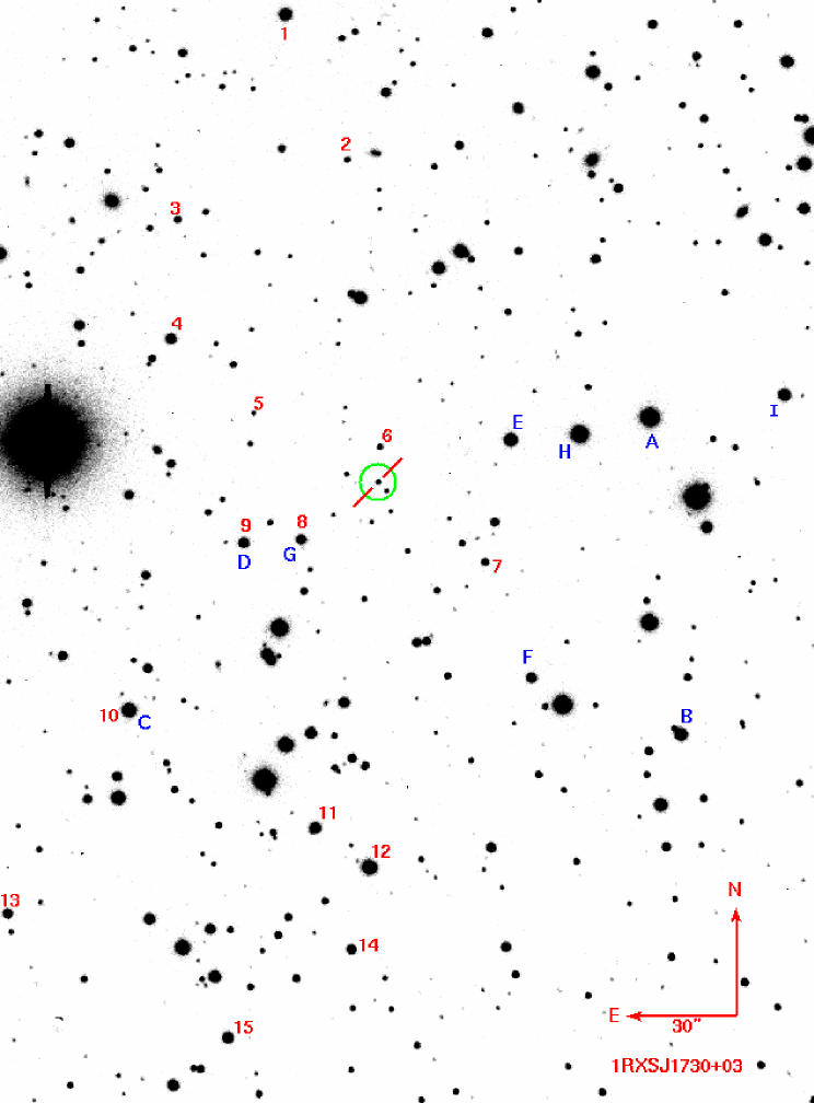
Figure 1.— Finder chart for 1RXS J1730+03 ($\alpha=17^{\rm h}$30^m06^s.19, $\delta=+03\arcdeg$38′18″.8). This i$\,{}^{\prime}$ band image was acquired with the Large Format Camera (LFC) at the 5 m Hale telescope at Palomar. Stars numbered 1–15 in red are used for relative photometry in LFC data. Stars labeled A–I in blue are used for relative photometry in P60 data (Section 2.1). The green circle shows the 5″ extraction region used for calculating UVOT fluxes. The circle includes a contaminator, 3″.4 to the South-West of the target.

The resultant lightcurves are shown in Figures 2, 3 & 4. Table 1 provides the photometry.

Table 3Observation Log for Swift ToO Observations of 1RXS J1730+03.

Obs ID	Start Date & Time	Stop Time	Exposure	Filter	Wavelength	Magnitude	Flux	Flux
			(s)		(Å)			($\mu$Jy)
00035571001	2006 Feb 9 16:56:43	18:42:00	1106	UVM2	2231	17.9$\pm$0.1	31$\pm$2	51$\pm$3
				XRT			0.02	0.06 (5 keV)
00031408001	2009 May 3 18:28:56	19:02:12	1964	UVM2	2231	20.44$\pm$0.21	3.04$\pm$0.59	5.05$\pm$0.99
00031408002	2009 May 4 18:34:04	22:12:54	4896	UVW1	2634	20.14$\pm$0.10	3.47$\pm$0.32	8.04$\pm$0.75
00031408003	2009 May 6 03:02:21	15:36:33	5621	UVW2	2030	21.48$\pm$0.17	1.38$\pm$0.22	1.93$\pm$0.30
				XRT			$<$0.002	$<$0.006 (5 keV)

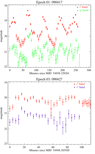
Figure 2.— P60 photometry of 1RXS J1730+03. Top panel: Epoch 1 photometry in g$\,{}^{\prime}$ and i$\,{}^{\prime}$ bands. Bottom panel: Epoch 3 photometry in r$\,{}^{\prime}$ and i$\,{}^{\prime}$ bands.

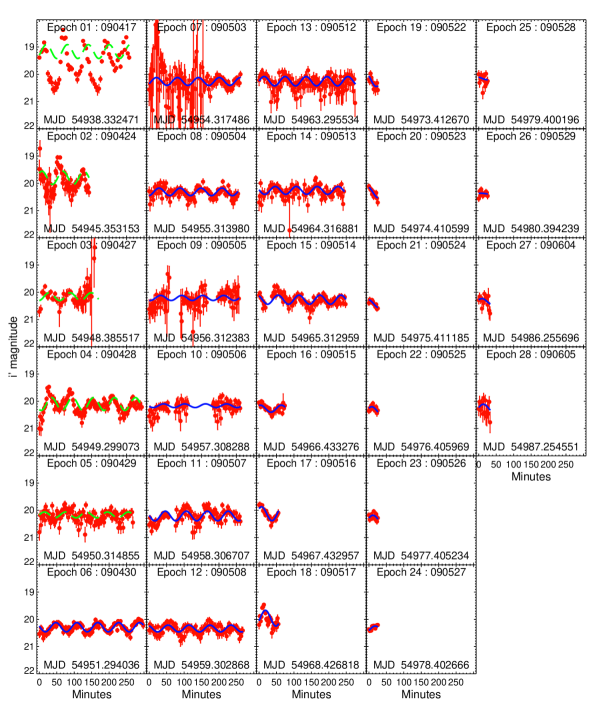
Figure 3.— i$\,{}^{\prime}$ band P60 photometry of 1RXS J1730+03, for Epochs 1 to 28. The source was in outburst in Epoch 1 and slowly faded into quiescence. The error bars denote relative photometry errors and do not include an absolute zero point error of 0.064 mag (§ 2.1). The solid blue line denotes the best fit sinusoid to the photometric data. The dashed green line is added to show the relative phase of the source in outburst, these epochs were not used for fitting the lightcurve.

2.2. Spectroscopy

We obtained optical and near-infrared spectra of 1RXS J1730+03 at various stages after outburst (Figure 5). The first optical spectra were taken 13 days after the first photometric epoch. We used the Low Resolution Imaging Spectrograph on the 10 m Keck-I telescope (LRIS; Oke et al., 1995), with upgraded blue camera (McCarthy et al., 1998; Steidel et al., 2004), covering a wavelength range from 3,200 Å – 9,200 Å. We acquired more optical data 34 days after outburst, with the Double Beam Spectrograph on the 5 m Hale telescope at Palomar (DBSP; Oke & Gunn, 1982). We took 5 exposures spanning one complete photometric period, covering the 3,500 Å – 10,000 Å wavelength range. We took late time spectra covering just over one photometric period for the quiescent source with the upgraded LRIS. At this epoch, we aligned the slit at a position angle of 45 degrees to cover both the target and the contaminator, 3″.4 to its South West (Figure 1). We also obtained low resolution $J$-band spectra with the Near InfraRed Spectrograph on the 10 m Keck-II telescope (NIRSPEC; McLean et al., 1998). 12 spectra of 5 minutes each were acquired, covering the wavelength region from 11,500 Å – 13,700 Å. For details of the observing set up, see the notes to Table 5.

We analyzed the spectra using IRAF and MIDAS and flux calibrated them using appropriate standards. Wavelength solutions were obtained using arc lamps and with offsets determined from sky emission lines. Figure 6 shows an optical spectrum from each epoch, while the IR spectrum is shown in Figure 7.

The second LRIS epoch had variable sky conditions. Here, we extracted spectra of the aforementioned contaminator. This object is also a M-dwarf, hence both target and contaminator spectra will be similarly affected by the atmosphere. We estimate the i$\,{}^{\prime}$ magnitude of the contaminator in each spectrum, and compare it to the the value measured from the LFC images to estimate and correct for the extinction by clouds.

2.3. X-ray and UV observations

We observed the 1RXS J1730+03 with the X-ray telescope (XRT) and the UV-Optical Telescope (UVOT) onboard the Swift X-ray satellite (Gehrels et al., 2004) during UT 2009 May 3-6 for a total of about 12.5 ks. The level-two event data was processed using Swift data analysis threads for the XRT (Photon counting mode; PC) using the HEASARC FTOOLS software package. The source was not detected in the X-ray band.

We follow the procedures outlined by Poole et al. (2008) for analyzing the UVOT data. The measured fluxes are given in Table 3. The contaminator is within the recommended 5^′′ extraction radius. Hence, flux measurements are upper limits.

Shevchuk et al. (2009) had observed 1RXS J1730+03 on UT 2006 February 9 with the Swift satellite as a part of investigations of unidentified ROSAT sources. They detected the source with a count rate of 0.02${\rm\,counts\,s}^{-1}$. The best-fit power law has a photon index $\Gamma=1.8\pm 0.5$ and a 0.5–10 keV flux of $1.2\times 10^{-12}\,{\rm erg\,cm^{-2}\,s^{-1}}$. After converting to the ROSAT bandpass assuming the XRT model parameters, this value is approximately a factor of two lower than the archival ROSAT flux. They report a much higher UV flux in their observations, which suggests that the source was in an active state during their observations.

The column density inferred from the XRT data is low, $N_{\rm H}\sim 7\times 10^{20}\,$cm^-2. From ROSAT data, this column density corresponds to $A_{\rm V}=0.39$, which gives $A_{\rm UVM2}=0.84$ (Cox, 2000). For comparison, Schlegel et al. (1998) give the Galactic dust extinction towards this direction ($l=26.^{\circ}7$, $b=19^{\circ}.7$) to be $E(B-V)=0.141$ mag ($A_{\rm V}=0.44$), corresponding to a column density of about $8\times 10^{20}\,{\rm cm}^{-2}$.

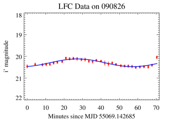
Figure 4.— i$\,{}^{\prime}$ band LFC photometry of 1RXS J1730+03 in quiescence, 131 days after we first saw high variability. The variations have the same phase and period as observed during outburst. See Figure 3 for details.

3. Nature of the components

The optical spectra (Figure 6) show rising flux towards the red and blue ends of the spectrum: indicative of a hot (blue) and cool (red) component. The red part of the spectrum shows clear molecular features, characteristic of late type stars. The blue component is devoid of any prominent absorption/emission features. From the overall spectral shape we infer that 1RXS J1730+03 is a CV.

3.1. Red component

The red component of 1RXS J1730+03 is typical of a late type star. In Figure 8, we compare the red side spectrum of 1RXS J1730+03 with several M-dwarfs. From the shape of the TiO bands at 7053 Å – 7861 Å, we infer that the spectral type to be M3$\pm$1. This is consistent with the relatively featureless J band spectrum (McLean et al., 2003). The spectral type indicates an effective temperature of 3400 K (Cox, 2000). The presence of a sodium doublet at 8183/8195 Å implies a luminosity class V.

We also fit the spectrum with model atmospheres calculated by Munari et al. (2005). For late type stars, these models are calculated in steps of $\Delta T=500{\rm\,K}$, $\Delta\log\,g=0.5$ and $\Delta{\rm[M/H]}=0.5$. We use model atmospheres with no rotational velocity $(V_{\rm rot}=0{\rm\,km\,s}^{-1})$ and convolve them with a kernel modeled on the seeing, slit size and pixel size. We ignore the regions contaminated by the telluric $A$ and $B$ bands (7615 Å and 6875 Å). The unknown contribution from the white dwarf was fit as a low order polynomial. We correct for extinction using $A_{\rm V}$ = 0.39 from X-ray data (Section 2.3). To measure $\log\,g$, we use the spectrum in the 8,000 Å – 8,700 Å region, which is expected to have fairly little contamination from the blue component. This region includes the Ca II lines at 8498, 8542 Å and the Na I doublet, which are sensitive to $\log\,g$. We then fit the spectra in the 6,700 Å – 8,700 Å range to determine the temperature and metallicity. The best fit model has ${\rm T}=3500{\rm\,K}$, $\log\,g=5.0$ and solar metallicity, consistent with our determination of the spectral type.

Kolb et al. (2001) state that unevolved donors in CVs follow the spectral type–mass relation of the zero age main sequence, as the effects of thermal disequilibrium on the secondary spectral type are negligible. For a M3 star, this yields a mass of $0.38\,M_{\odot}$. As the secondaries evolve, the spectral type is no longer a good indicator of the mass and gives only an upper limit on the mass. The lower limit can simply be assumed to be the Hydrogen-burning limit of $0.08\,M_{\odot}$.

Table 4Locations of Cyclotron Harmonics.

Harmonic	Measured	Measured	Inferred
number	Wavelength	Frequency	Wavelength
	(Å)	(Hz)	(Å)
7	3540	$8.4\times 10^{14}$	3664
6	4440	$6.7\times 10^{14}$	4275
5	5180	$5.7\times 10^{14}$	5130
4	6770	$4.4\times 10^{14}$	6413
3	8225	$3.6\times 10^{14}$	8551
2	$\cdots$	$\cdots$	12826
1	$\cdots$	$\cdots$	25653

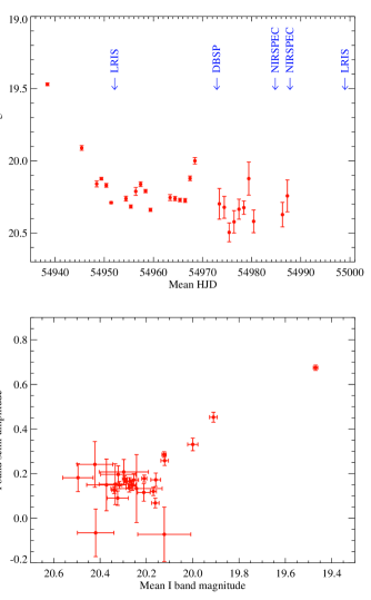
Figure 5.— Photometric evolution of 1RXS J1730+03 in i$\,{}^{\prime}$ band. Data for each epoch was fit with a sinusoid with the same period for all epochs. In contrast to Figures 3 & 4, the phase was allowed to vary independently for each epoch. Top: average i$\,{}^{\prime}$ magnitude for each P60 observation epoch, as a function of time. Blue arrows mark spectroscopy epochs. Bottom: semi-amplitude of sinusoidal variations as a function of the corresponding mean i$\,{}^{\prime}$ magnitudes for each epoch.

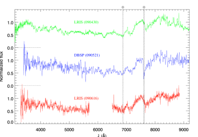
Figure 6.— Temporal evolution of 1RXS J1730+03 spectra. Some spectra are not corrected for Telluric absorption, the affected regions are diagonally hatched. The first spectrum was obtained 13 days after we measured high variability, the second after 34 days, and the lowermost spectrum after 60 days. The spectra show broad Balmer features which evolve with time. The M-dwarf features (TiO, Na I) are clearly seen at all times.

3.2. Blue component

The blue component of 1RXS J1730+03 is consistent with a highly magnetic white dwarf. The blue spectrum is suggestive of a hot object, but does not show any prominent absorption/emission features. H$\alpha$ is seen in emission, but other Balmer features are not detected. The spectrum (Figure 6) shows cyclotron humps, suggesting the presence of a strong magnetic field. The polar nature of the object is supported by the absence of an accretion disc, and the transition from an active state to an off state in X-rays (Section 1, Section 2.3).

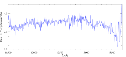
Figure 7.— Keck NIRSPEC spectrum of 1RXS J1730+03. The spectrum is flat and nearly featureless, as expected for early M stars.

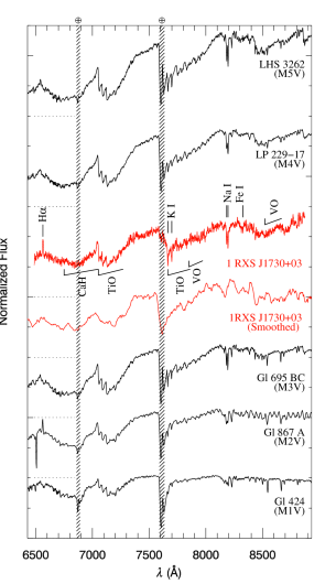
Figure 8.— Comparison of red part of 1RXS J1730+03 spectrum with M-dwarf spectra. Some spectra are not corrected for Telluric absorption, the affected regions are diagonally hatched. Prominent bands (TiO, CaH) and lines (H$\alpha$, Na I) are marked. Comparing the shape of the TiO bands at 7053–7861 Å and the shape of the continuum redwards of 8200 Å, we infer that spectral type of the red component to be M3. The presence of a sodium doublet at 8183/8195 Å implies a luminosity class V.

For analyzing the WD spectrum, we subtracted a scaled spectrum of the M-dwarf GL 694 from the composite spectrum of 1RXS J1730+03. The resultant spectrum (Figure 9) clearly shows cyclotron harmonics. The hump seen in the J-band spectrum (Figure 7) is also inferred to be a cyclotron harmonic. A detailed modeling of the magnetic field is beyond the scope of this work, but we use a simple model to estimate the magnetic field. We fit the cyclotron humps with Gaussians and measure the central wavelengths (Table 4). We then fit these as a series of harmonics, and infer that the cyclotron frequency is $\nu_{\rm cyc}=1.17\times 10^{14}{\rm\,Hz}$. The magnetic field in the emission region is given by, $B=(\nu_{\rm cyc}/2.8\times 10^{14}{\rm\,Hz})\cdot 10^{8}{\rm\,G}=42\times 10^{6}{\rm\,G}$.

As a conservative error estimate, we consider the worst case scenario where our identified locations for the cyclotron humps are off by half the spacing between consecutive cyclotron harmonics. Using this, we estimate the errors on the magnetic field: $B=42^{+6}_{-5}{\rm\,MG}$.

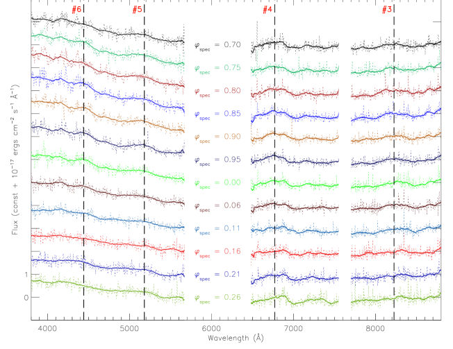
Figure 9.— Blue component spectra of 1RXS J1730+03, showing the 12 late-time LRIS exposures (Section 2.2, Table 5). The spectroscopic phase at mid-exposure is indicated for each spectrum. Dotted lines show spectra are obtained by subtracting a scaled spectrum of GL 694 from spectra of this binary. The overlaid solid lines are smoothed versions of the same spectra. Vertical dashed cyclotron humps at 4440 Å, 5180 Å, 6770 Å & 8225 Å. The cyclotron harmonic numbers (#3 – #6) are indicated in bold red. Two more cyclotron humps are seen in other spectra: a feature at 3540 Å (Figure 6), and a $J$-band feature (Figure 7).

4. System parameters

4.1. Orbit

We use the best fit Munari et al. (2005) model atmosphere to measure radial velocities of the M-dwarf. We vary the radial velocity of the model, and minimize the $\chi^{2}$ over the 6,500 Å – 8,700 Å spectral region, excluding the telluric O₂ bands. After a first iteration, the spectra are re-fit to account for motion of the M-dwarf during the integration time. For the 12 spectra taken at the second LRIS epoch, we also measure the radial velocity for the contaminator star on the slit, and find it to be constant. This serves as a useful test for our radial velocity measurement procedure. The barycentric corrected velocities are given in Table 5.

We fit a circular orbit ($v_{2}=\gamma_{2}+K_{2}\sin([2\pi(t-t_{0})]/P)$) to the measured velocities. We define the superior conjunction of the WD as phase 0.

The 2009 June 16 spectroscopic data (Table 5) give an orbital period $P_{\rm est}=123\pm 3{\rm\,min}$. We then use the photometric variability (Section 4.2) to determine an accurate period in this range. Next, we refine the solution with velocity measurements from the other two spectroscopic epochs. The best-fit solution gives a period $P=120.2090\pm 0.0013{\rm\,min}$ and $K_{2}=390\pm 4{\rm\,km\,s}^{-1}$ (Table 6, Figure 10).

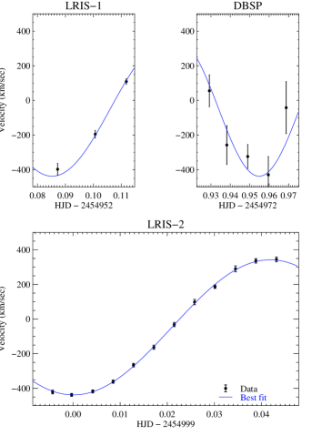
Figure 10.— Velocity measurements 1RXS J1730+03. The best-fit solution gives $P=120.2090\pm 0.0013{\rm\,min}$, $\gamma_{2}=-48\pm 5{\rm\,km\,s}^{-1}$ and $K_{2}=390\pm 4{\rm\,km\,s}^{-1}$ (Section 4.1)

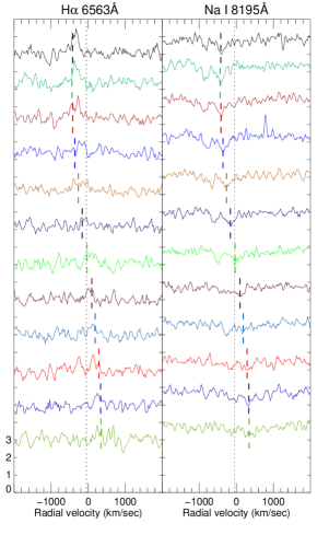
Figure 11.— Velocity modulation of H$\alpha$ and the 8184/8195 Å Na I doublet. The spectra are offset by $2\times 10^{-17}\,{\rm erg\,cm^{-2}\,s^{-1}}$ for clarity. The wavelengths are converted into velocities using the rest wavelengths 6563 Å and 8195 Å respectively. The vertical dotted line marks the radial velocity of the binary barycenter. The short dashed lines mark the radial velocities measured by fitting the complete spectrum. The Na I absorption follows the radial velocity of the M-dwarf, but H$\alpha$ seems to have a smaller velocity amplitude.

Figure 11 shows sections of the last epoch spectra around H$\alpha$ and the Na I doublet at 8184/8195 Å. The Na I doublet clearly matches the velocity of the M-dwarf in the orbit, but the H$\alpha$ emission seems to have a smaller velocity amplitude. A possible explanation for this is that the H$\alpha$ emission comes from the M-dwarf surface that is closest to the WD, which may be heated by emission from the white dwarf or the accretion region.

Table 5Radial velocity of the M-dwarf.

Heliocentric JD	Exposure time	Barycentri	Instrument
		Radial Velocity
	(s)	(${\rm\,km\,s^{-1}}$)
2454952.08721	1020	$-398\pm 34$	LRIS
2454952.10067	1020	$-195\pm 22$	LRIS
2454952.11179	600	$109\pm 16$	LRIS
2454972.92923	600	$55\pm 92$	DBSP
2454972.93818	900	$-258\pm 112$	DBSP
2454972.94896	900	$-324\pm 69$	DBSP
2454972.95956	900	$-430\pm 105$	DBSP
2454972.96875	600	$-42\pm 150$	DBSP
2454998.99566	210	$-421\pm 11$	LRIS
2454998.99969	300	$-438\pm 9$	LRIS
2454999.00418	300	$-417\pm 9$	LRIS
2454999.00850	300	$-361\pm 9$	LRIS
2454999.01283	300	$-266\pm 10$	LRIS
2454999.01715	300	$-163\pm 12$	LRIS
2454999.02147	300	$-32\pm 12$	LRIS
2454999.02580	300	$98\pm 15$	LRIS
2454999.03012	300	$186\pm 10$	LRIS
2454999.03448	300	$290\pm 17$	LRIS
2454999.03880	300	$336\pm 13$	LRIS
2454999.04317	300	$344\pm 13$	LRIS

Table 6Orbital Velocity Parameters of the M-dwarf.

Parameter	Value
$\gamma_{2}$ (${\rm\,km\,s^{-1}}$)	$-48\pm 5$
$K_{2}$ (${\rm\,km\,s^{-1}}$)	$390\pm 4$
$t_{0}$ (HJD)	$54998.9375\pm 0.0003$
$P$ (min)	$120.2090\pm 0.0013$

4.2. Photometric Variability

The lightcurve of 1RXS J1730+03 shows clear periodicity (Figures 2 – 4), with two peaks per spectroscopic period. Most of the photometric data was acquired in the i$\,{}^{\prime}$ band, which contains contribution from both the M-dwarf and a cyclotron harmonic from the emission region near the WD.

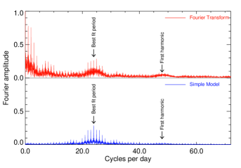
Figure 12.— Upper panel: Fourier transform of all i$\,{}^{\prime}$ data. Lower panel: expected Fourier transform for a pure sinusoidal variations with a period of 60.11 min, obtained by scaling and convolving the Fourier transform of the window function with a delta function corresponding to the best-fit period.

A Fourier transform of the data (Figure 12) shows a strong peak at sixty minutes. We interpret this as a harmonic of the orbital period. To determine the exact period, we analyze the data as follows. As the object has a short orbital period, we convert all times to Heliocentric Julian Date for analysis. We fit a sinusoid ($m_{0}+m_{A}\sin([2\pi(t-t_{0})]/P)$) to each epoch, allowing $m_{0}$ and $m_{A}$ to vary independently for each epoch, but we use the same reference time $t_{0}$ and period $P$ for the entire fit. The mean magnitude is correlated with the amplitude (Figure 5). Note that the amplitude measured for the sinusoidal approximation for each epoch is always less than the actual peak-to-peak variations of the source during that epoch, as expected. The source is in the active state in the first few epochs, and we exclude epochs 1 – 5 from the fit, to avoid contamination from the accretion stream and/or the accretion shock.

The best-fit solution is overplotted in blue in Figures 3 & 4. Since epochs 1 – 5 were not included in the fit, a sinusoid is overplotted in dashed green to indicate the expected phase of the variations. The best-fit period is $60.1059\pm 0.0005$ minutes. This formally differs from the spectroscopically determined orbital period by $2.1\sigma$. However, this error estimate includes only statistical errors. There is some, difficult to determine, systematic error component in addition, so we do not claim any significant inconsistency.

Periodic photometric variability for 1RXS J1730+03 can be explained as a combination of two effects: cyclotron emission from the accretion region and ellipsoidal modulation. The active state is characterized by a higher mass transfer rate from the donor to the WD, and results in higher cyclotron emission. This emission is beamed nearly perpendicular to the magnetic field lines, creating an emission fan beam. For high inclination systems, the observer crosses this fan beam twice, causing two high amplitude peaks per orbit (Figure 2). In the active state when the emission is dominated by cyclotron radiation, the minimum leads the superior conjuntion by $\sim 47$°.

In ellipsoidal modulation, and the photometric minima coincide with the superior conjunction. It is observed that in quiescence, the photometric minimum leads the superior conjunction of the white dwarf by $\sim 14$°. This suggests that the $0.29\pm 0.13$ mag variation is caused by a combination of ellipsoidal modulation and cyclotron emission from the accretion region.

4.3. Mass Ratio

The semi-amplitude of the M-dwarf radial velocity, K2, gives a lower limit on the mass of the white dwarf. For a circular orbit, one can derive from Kepler’s laws that:

$$M_{1,{\rm min}}=\frac{PK_{2}^{3}}{2\pi G}=0.52\,M_{\odot}$$ (1)

Tighter constraints can be placed on the individual component masses $M_{1}$, $M_{2}$ by considering the geometry of the system. Eggleton (1983) expresses the volume radius $R_{2}$ of the secondary in terms of the mass ratio $q=M_{2}/M_{1}$:

$$\frac{R_{2}}{a}=\frac{0.49q^{2/3}}{0.6q^{2/3}+\ln(1+q^{1/3})}$$ (2)

where the separation of the components is given by $a=[P^{2}G(M_{1}+M_{2})/4\pi^{2}]^{1/3}$ . Thus for a fixed period $P$, $R_{2}$ depends only on $M_{2}$. The radius of the white dwarf is much smaller than that of the M-dwarf. Hence, the M-dwarf will eclipse the accretion region if the inclination of the system is $i<\sin^{-1}(R_{2}/a)$. Figures 3, 4 show that we do not detect any eclipses in the system.

Figure 13 shows the allowed region for 1RXS J1730+03 in a WD mass – M-dwarf mass phase space. The orange dotted region is excluded as the orbital velocity would be greater than the measured projected velocity. The red hatched region is excluded by non-detection of eclipses. The allowed mass of the primary ranges from the minimum mass ($M_{1}>0.52\,M_{\odot}$) to the Chandrashekhar limit. The mass of the secondary is bounded above by the ZAMS mass for a M3 dwarf ($M_{2}=0.38\,M_{\odot}$).

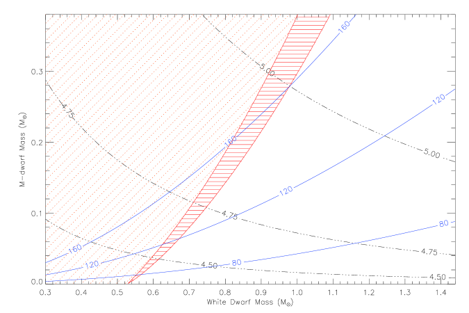
Figure 13.— The allowed range of masses (clear white region) for components of 1RXS J1730+03. The orange dotted region is excluded by the minimum inferred masses from radial velocity measurements. The red hashed region is excluded by non-detection of eclipses (Figures 3, 4). The black dash-dot lines show contours of constant $\log\,g$. The best fit spectra yeild $\log\,g=5.0$. The solid blue lines are calculated contours for the rotation velocity (km s^-1) of the M-dwarf. A measurement of $v\sin i$ will help to constrain masses of the components.

For a given $M_{2}$ and a known orbital period, we can determine the radius of the secondary using Equation (2), and can calculate the surface gravity ($\log\,g$). For $0.38\,M_{\odot}\gtrsim M_{2}\gtrsim 0.05\,M_{\odot}$, $\log\,g$ ranges from 5.1 to 4.8. This is consistent with $\log\,g=5.0$ for the best fit M-dwarf spectrum (Section 3.1).

The donor stars in CVs are expected to co-rotate. For 1RXS J1730+03, the highest possible rotational velocity $v\sin i$ is $\sim\,160{\rm\,km\,s}^{-1}$ for a $0.38\,M_{\odot}$, $0.27\,R_{\odot}$ M-dwarf and a $1.1\,M_{\odot}$ WD (Figure 13). $v\sin i$ will be lower if the WD is heavier or if the M-dwarf is lighter. To measure rotational broadening in the spectra, we use a higher resolution ($R=20,000$) template of the best-fit model from Zwitter et al. (2004). We take a template with zero rotation velocity and broaden it to different rotational velocities using the prescription by Gray (2005). Then we use our fitting procedure (Section 3.1) to find the best-fit value for $v\sin i$. For this measurement, we use only the 12 relatively high resolution spectra from the second LRIS epoch (UT 2009 June 16). The weighted $v\sin i$ from the twelve spectra is $97\pm 22{\rm\,km\,s}^{-1}$, but the measurements show high scatter, with a standard deviation of $54{\rm\,km\,s}^{-1}$. We compared our broadened spectra with rotationally broadened spectra computed by Zwitter et al. (2004), and found that our methods systematically underestimate $v\sin i$ by $\sim\,20{\rm\,km\,s}^{-1}$. We do not understand the reason for this discrepancy, hence do not feel confident enough to use this value in our analysis. A reliable measurement of $v\sin i$ will help better constrain the masses of the two components.

4.4. Distance

We estimate the distance to 1RXS J1730+03 as follows. Our fitting procedure (Section 3.1) corrects for extinction and separates the WD and M-dwarf components of the spectra. We correct for varying sky conditions by using a reference star on the slit. The ratio of measured flux to the flux of the best fit model atmosphere ($T=3500{\rm\,K},\log g=5.0$) is,

$$\frac{f_{\rm measured}}{f_{\rm model}}=\left(\frac{R_{2}}{d}\right)^{2}=(6.1\pm 1.6)\times 10^{-23}$$ (3)

where $d$ is the distance to the source, and $R_{2}$ is given by Equation (2).

For 1RXS J1730+03, the maximum mass of the M-dwarf is $0.38\,M_{\odot}$, and the corresponding radius is $R_{2}=0.27\,R_{\odot}$. Equation (3) then gives $d=800\pm 110{\rm\,pc}$. This calculation assumes the largest possible M-dwarf radius, hence is an upper limit to distance. If the M-dwarf is lighter, say $0.1\,M_{\odot}$, we get $R_{2}=0.17\,R_{\odot}$, yielding $d=500\pm 70{\rm\,pc}$.

5. Conclusion

1RXS J173006.4+033813 is a polar cataclysmic variable, similar to known well-studied systems like BL Hyi, ST LMi and WW Hor in terms of the orbital period, magnetic field and variability between active and quiescent states. This source is notable for the highly symmetric nature and high amplitude of the double–peaked variation in the active state. This suggests a relatively high angle between the rotation and magnetic axes. Polarimetric observations of the source would help to better constrain the magnetic field geometry of the system.

Most polars are discovered due to their highly variable X-ray flux. However, we mounted a followup campaign for 1RXS J1730+03 due to its unusual optical variability properties. This suggests that current and future optical synoptic surveys, such as PTF (Law et al., 2009) and LSST can uncover a large sample of polars by cross-correlating opticaly variable objects with the ROSAT catalog.

References

- Blackburn (1995) Blackburn, J. K. 1995, Astronomical Data Analysis Software and Systems IV, 77, 367
- Cenko et al. (2006) Cenko, S. B., et al. 2006, PASP, 118, 1396
- Cox (2000) Cox, A. N. 2000, Allen’s Astrophysical Quantities, Springer, Berlin, 2000, 4 edn.
- Cropper (1990) Cropper, M. 1990, Space Science Reviews, 54, 195
- Denisenko et al. (2009) Denisenko, D. V., Kryachko, T. V., & Satovskiy, B. L. 2009, The Astronomer’s Telegram, 2014, 1
- Eggleton (1983) Eggleton, P. P. 1983, ApJ, 268, 368
- Gehrels et al. (2004) Gehrels, N., et al. 2004, ApJ, 611, 1005
- Gray (2005) Gray, D. F. 2005, The Observation and Analysis of Stellar Photospheres, 3rd Edition, by D.F. Gray. ISBN 0521851866. http://www.cambridge.org/us/catalogue/catalogue.asp? isbn=0521851866. Cambridge, UK: Cambridge University Press, 2005.,
- Hellier (2001) Hellier, C. 2001, Springer-Praxis books in Astronomy & Space Sciences, Chichester, UK
- Hellier (2002) Hellier, C. 2002, in The Physics of Cataclysmic Variables and Related Objects, ed. B. T. Gänsicke, K. Beuermann, & K. Reinsch, ASP Conf. Ser., 261, 92
- Kolb et al. (2001) Kolb, U., King, A. R., & Baraffe, I. 2001, MNRAS, 321, 544
- Landsman (1993) Landsman, W. B. 1993, Astronomical Data Analysis Software and Systems II, 52, 246
- Law et al. (2009) Law, N. M., et al. 2009, PASP, 121, 1395
- McCarthy et al. (1998) McCarthy, J. K., et al. 1998, Proc. SPIE, 3355, 81
- McLean et al. (2003) McLean, I. S., McGovern, M. R., Burgasser, A. J., Kirkpatrick, J. D., Prato, L., & Kim, S. S. 2003, ApJ, 596, 561
- McLean et al. (1998) McLean, I. S., et al. 1998, Proc. SPIE, 3354, 566
- Mighell (1999) Mighell, K. J. 1999, Astronomical Data Analysis Software and Systems VIII, 172, 317
- Munari et al. (2005) Munari, U., Sordo, R., Castelli, F., & Zwitter, T. 2005, A&A, 442, 1127
- Oke & Gunn (1982) Oke, J. B., & Gunn, J. E. 1982, PASP, 94, 586
- Oke et al. (1995) Oke, J. B., et al. 1995, PASP, 107, 375
- Poole et al. (2008) Poole, T. S., et al. 2008, MNRAS, 383, 627
- Ramsay et al. (2004) Ramsay, G., Cropper, M., Wu, K., Mason, K. O., Córdova, F. A., & Priedhorsky, W. 2004, MNRAS, 350, 1373
- Schlegel et al. (1998) Schlegel, D. J., Finkbeiner, D. P., & Davis, M. 1998, ApJ, 500, 525
- Shevchuk et al. (2009) Shevchuk, A. S., Fox, D. B., Turner, M., & Rutledge, R. E. 2009, The Astronomer’s Telegram, 2015, 1
- Simcoe et al. (2000) Simcoe, R. A., Metzger, M. R., Small, T. A., & Araya, G. 2000, Bulletin of the American Astronomical Society, 32, 758
- Steidel et al. (2004) Steidel, C. C., Shapley, A. E., Pettini, M., Adelberger, K. L., Erb, D. K., Reddy, N. A., & Hunt, M. P. 2004, ApJ, 604, 534
- Voges et al. (1999) Voges, W., et al. 1999, A&A, 349, 389
- Warner (1995) Warner, B. 1995, Cambridge Astrophysics Series, Cambridge, New York: Cambridge University Press, —c1995,
- Zwitter et al. (2004) Zwitter, T., Castelli, F., & Munari, U. 2004, A&A, 417, 1055