Study of multi black hole and ring singularity
apparent horizons

Abstract

We study critical black hole separations for the formation of a common apparent horizon in systems of $N$ - black holes in a time symmetric configuration. We study in detail the aligned equal mass cases for $N=2,3,4,5$, and relate them to the unequal mass binary black hole case. We then study the apparent horizon of the time symmetric initial geometry of a ring singularity of different radii. The apparent horizon is used as indicative of the location of the event horizon in an effort to predict a critical ring radius that would generate an event horizon of toroidal topology. We found that a good estimate for this ring critical radius is $20/(3\pi)M$. We briefly discuss the connection of this two cases through a discrete black hole ’necklace’ configuration.

1 Introduction

The field of Numerical Relativity (NR) has progressed rapidly since the 2005 breakthroughs [1, 2, 3]. Naturally, the first application of these techniques was to solve the non-linear dynamics of the inspiral, merger, and ringdown of an orbiting black-hole binary (BHB). The computation of the gravitational waveforms generated by such systems is of utter interest for gravitational wave observatories such as LIGO, VIRGO and LISA. The computation of the merger of BHB is also of astrophysical interest. In particular, the discovery of very large recoil velocities [4, 5] acquired by the final remnant of the merger has attracted lots of interest among astrophysicists.

There are other very important applications of the new NR techniques. Those lie in the field of Mathematical Relativity. Some few examples are given by the studies of the geometry of maximally spinning black holes [6, 7] behaving like $1/\sqrt{r}$ rather than $1/r$ for submaximal near the puncture. The late time behavior of the metric conformal factor in the ’moving puncture’ approach also behavs like [8, 9, 10, 11] $1/\sqrt{r}$. Numerical simulations started to test the ’no hair’ theorem [12] and the ’cosmic censorship’ conjecture [13, 14]. The isolated horizon formalism [15] has been implemented numerically and validated in highly nonlinear regimes. In particular a new proposal to measure quasilocally linear momenta from the horizon deformation of black holes has been put forward in [16]. In this paper we turn into the study of the merging of apparent horizon of $N$-black hole systems and a ring singularity in a time symmetric initial geometry. These studies can be used as a guide to search for event horizons in more dynamical situations.

In the next subsections we review basic definitions that will help us define and study apparent horizons for systems of $N$ black holes and black hole rings. We start with the definition of an event horizon and continue with apparent horizons, the equations used to find them and a basic summary of the algorithms used in this project to solve these equations. A follow up paper [17] will deal with the event horizon studies.

In Sec. 2 we study systems of $N$ aligned Schwarzschild black holes in a time-symmetric spacelike hypersurface. The equations involved and the numerical methods used are presented and explained. Additionally, the relationship between a system of two black holes of different mass and systems of $N$ black holes with equal mass is explored.

In section 3 we take advantage of the equations used for systems of $N$ black holes and adapt them to find the apparent horizon of a black hole with a rings singularity of different mass (or equivalently keeping constant the total mass and changing the radius.) This allows us to confirm that they comply with the results obtained by Galloway [18] regarding the spherical topology of apparent horizons in stationary black holes spacetimes. Additionally, the apparent horizon is used as an approximation to the event horizon and extrapolation is used to determine the size of the black hole ring that would give rise to an event horizon of toroidal topology. We end with a discussion of the possibility of building up a toroidal black hole with a discrete set of black holes in a ring-like distribution.

1.1 Definitions:

In an asymptotically flat spacetime the black hole region is a region from which no null curve can reach future null infinity ($\mathscr{I^{+}}$ ), the boundary of this region is the event horizon. Since the black hole region only ceases to increase when no more matter falls into it, its boundary cannot be determined until all interactions between the black hole and the surrounding matter are over. This means that in order to find the event horizon one must complete a full simulation of the evolution of the black hole. A more local structure such as an apparent horizon provides a way to overcome this requirement. Since the existence of an apparent horizon is a necessary condition for the existence of an event horizon and because an apparent horizon will always lie inside an event horizon, these objects have become very useful in numerical relativity. In fact there are certain algorithms that make use of “horizon pretracking”, more fully described in [19], or “black hole excision techniques” [20, page 214], where the goal is to find the apparent horizons as soon as they appear in a simulation in order to remove the singularity and measure the mass and angular momentum of the black hole .

Now, there are certain cases where the problem of finding the event horizon can be simplified. For example when we are working in stationary, asymptotically flat spacetimes, the event horizon is a null three surface $H$, tangent to one or more Killing vector fields of the full spacetime. These types of horizons are formally known as Killing horizons. On the other hand, If the Killing vector field is not of the full spacetime, but rather of some neighborhood of the null three surface H, then the Killing Horizon does not coincide with the event horizon, but it is close to it [21].

Still, apparent horizons are, for the most part, the best way to locate a black hole. But before defining what exactly is an apparent horizon we need to define first a trapped surface. Booth describes for Kerr-Newman black holes the trapped surface as a closed two-surface $S$ with the property that all null geodesics that are normal to the surface and are pointing forward in time have negative expansion everywhere [21]:

$$\theta(l)=q^{ab}\nabla_{a}l_{b}<0\quad\textrm{and}\quad\theta(n)=q^{ab}\nabla_{a}n_{b}<0$$ (1)

Here $q_{ab}=g_{ab}+l_{a}n_{b}+l_{b}n_{a}$ is the two metric induced on $S$ and $l^{a}$ , $n^{a}$ are the outward, inward pointing null directions with $l\cdot n=-1$.

Then, given a spacetime that can be foliated into hypersurfaces $\Sigma_{t}$, a point $q\in\Sigma_{t}$ is said to be trapped if it lies on a trapped surface of $\Sigma_{t}$. An apparent horizon is the boundary of the union of all trapped points. When this boundary is differentiable, the apparent horizon is a marginally outer trapped surface, MOT ( $\theta(l)=0$). In other words, the apparent horizon is a trapped surface in which light rays have zero expansion in the null directions that are normal to the surface. It is this definition of an apparent horizon that has helped develop algorithms to find it. The one used in this project is based on the description of ” shooting algorithms in axisymmetry” by Thornburg [19] and Bishop [22, 23].

In the process of finding apparent horizons for systems of $N$ black holes, we find that there is a certain distance between black holes that creates a common apparent horizon. We will refer to this distance as the critical separation $a_{c}$. For example, if two black holes are at a distance $a_{c}$ or less from each other then a common apparent horizon will form between them. On the other hand, if the two black holes are at a distance greater than $a_{c}$ then two apparent horizon will form, each surrounding one of the two black holes.

1.2 Motivation

As mentioned before, the event horizon represents the true boundary of the black hole. However, in order to find it we need to know which outgoing null rays escape to infinity and which ones do not. They only way to achieve this is by knowing the entire history of the spacetime. This requires a complete simulation of the evolution of the black hole. That is why locating the apparent horizon is so important in Numerical Relativity. It represents a local boundary for the black hole region and provides physical information about the black hole such as mass and angular momentum. They are also used in numerical simulations to locate the black holes so that black hole excision techniques can be used. It is for these reasons that we have focused our research in apparent horizons.

On the other hand, during the past few years system of three black holes have been studied [24, 25, 26, 27]. Moreover, the good probability of finding systems of three or even more black holes [28] in globular clusters has motivated us to consider methods for the general case of $N$ black holes. As a starting point for more in depth future research we have restricted ourselves to the stationary axisymmetric case.

As an extension to the methods developed in the the study of $N$ black holes we also consider black hole rings. The paper [29] proving the existence of toroidal event horizons in rotating clusters of toroidal configuration motivated us to study these black hole rings. In this case we have considered the apparent horizon as an approximation to the event horizon. The effects of changing the mass of the black hole ring on the shape of the apparent horizon are studied. The results were tabulated in order to make a prediction about of topology of the event horizon.

1.3 Finding Apparent Horizons

The problem of finding an apparent horizon assuming an axisymmetric spacetime can be reduced to solving a non linear boundary value problem, as described in the following paragraphs. Then a numerical method can be used to solve this boundary value problem. The following derivation of the equations needed to find an apparent horizon in an axisymmetric case is a summary of the methods described in [20, pages 221-226], and can be found there in more detail.

Consider a spacetime manifold $M$ with metric $g_{\alpha\beta}$ and a spacelike hypersurface $\Sigma$ in this manifold. Let $\gamma_{ij}$ be the induced metric on the hypersurface $\Sigma$ and $K_{ij}$ be the extrinsic curvature. Here is worth mentioning the distinction between intrinsic curvature and extrinsic curvature. The intrinsic curvature of a hypersurface comes from its internal geometry and is given by the three dimensional Riemann tensor defined in terms of the metric $\gamma_{ij}$. The extrinsic curvature on the other hand is associated with the way these hypersurfaces are embedded in spacetime. It describes how the normal vector to the surfaces changes as its parallel transported from one point to the other. This change is described by the extrinsic curvature tensor $K_{ij}$ [20] 69.

In this hypersurface consider a smooth 2D surface $S$ embedded in it with a unit outward pointing normal vector $n^{\mu}$. Then the expansion, $\theta$, of null rays which are moving in the $n^{\mu}$ direction of $S$ is given by:

$$\theta=\nabla_{i}n^{i}+K_{ij}n^{i}n^{j}+K$$ (2)

Where $K$ is the trace of the extrinsic curvature $K_{ij}$ and $\nabla_{i}$ is the covariant derivative with respect to the metric $\gamma_{ij}$. As mentioned before the apparent horizon is a marginally trapped surface therefore it will be the surface for which $\theta=0$.

If the surface is parametrized by a level set (a surface for which the time coordinate is a constant) :

$$F(x^{i})=0$$ (3)

Then the normal vector to this surface is just the gradient of F:

$$n^{i}=\frac{\nabla^{i}F}{|\nabla F|}$$ (4)

Plugging equation 4 into equation 2 we obtain the following:

$$\theta=\frac{\gamma^{ij}\nabla_{i}F\nabla_{j}F}{|\nabla F|}-\frac{\nabla^{i}F\nabla^{j}F\nabla_{i}\nabla_{j}F}{|\nabla F|^{3}}+K_{ij}\frac{\nabla^{i}F\nabla^{j}}{|\nabla F|^{2}}+K$$ (5)

Then the level set curve that satisfies $\theta=0$ would be the apparent horizon. In the case of axisymmetric space, which is the case we are considering, the level surface can be expressed as:

$$F(r,\phi)=r-h(\phi)$$ (6)

This parameterization implies that we are considering apparent horizons which have a center and rays leaving this center will intersect the apparent horizon only once. In other words the parameterization assumes that the apparent horizon has a spherical topology. Another assumption is that the apparent horizon must be a smooth surface. This assumption suggests that when $\phi=0$ and $\phi=\pi$ we have $\partial_{\phi}h=0$

In his papers [22], [23] Bishop assumes that the extrinsic curvature $K_{ij}$ is zero. This simplification can be done because we are working in a time symmetric hypersurface and so the black holes are not moving in this time slice. Hence the equation for the expansion reduces to:

$$\theta=\nabla_{i}n^{i}$$ (7)

This implies that under these conditions the apparent horizon is an extremal (minimal) surface. Hence, it is possible to find the apparent horizon by finding a surface in $\Sigma$ of minimal area. This method is described in the next section.

2 Systems of N black holes in a line

This section is concerned with finding the apparent horizon for systems of $N$ black holes. First a system of two black holes of different mass is analyzed. A table relating the mass ratio of the two black holes and their critical separation is reproduced. Then systems of three, four and five black holes are considered. These systems are treated as if they contained only two black holes by grouping the black holes adequately. The table is then used to make a prediction about the location of the apparent horizon of these systems. These predictions are then compared to the actual location of the apparent horizon obtained using Bishop’s equations [22]. Finally a method for finding an approximation of the apparent horizon of a system of $N$ black holes, by representing it as a system of two black holes of different mass, is developed.

2.1 Equations

The equations used to find the apparent horizon are presented in references [29], [22] and [23]. A summary of the method is given here. It was assumed that the spacelike slice is a time-symmetric hypersurface with axial symmetry. In cylindrical coordinates the hypersurface has the following metric:

$$ds^{2}=\Psi^{4}(d\rho^{2}+\rho^{2}d\theta^{2}+dz^{2})$$ (8)

Assuming G=c=1 and with:

$$\Psi=1+\sum_{i}\frac{m_{i}}{2R_{i}}$$ (9)

Here $R_{i}=r-r_{i}$ is the difference between a reference point $r=(\rho,z)$ and the location of the $i^{th}$ black hole $r_{i}=(\rho_{i},z_{i})$.

As mentioned in the introduction the apparent horizon is a marginally outer trapped surface. Given the assumption that we are working in a time symmetric hypersurface (the black holes are not moving in this time slice) this implies that the intrinsic curvature $K_{ij}=0$. Hence the equation for the expansion of null rays normal to the surface is:

$$\theta=\nabla_{i}n^{i}$$ (10)

This implies that for this particular case finding marginally trapped surfaces is equal to finding extremal surfaces. Since extremal surfaces have minimal area we are looking to minimize the following:

$$\lambda=\int 2\pi\rho\Psi^{2}[\Psi^{4}dz^{2}+\Psi^{4}d\rho^{2}]^{1/2}$$ (11)

This can be rewritten as:

$$\lambda=\int 2\pi\rho\Psi^{2}[\Psi^{4}\left(\frac{dz}{d\sigma}\right)^{2}+\Psi^{4}\left(\frac{d\rho}{d\sigma}\right)^{2}]^{1/2}d\sigma$$ (12)

After the following transformation $Q=\rho\Psi^{4}$ we obtain:

$$\lambda=\int 2\pi[Q^{2}\left(\frac{dz}{d\sigma}\right)^{2}+Q^{2}\left(\frac{d\rho}{d\sigma}\right)^{2}]^{1/2}d\sigma$$ (13)

Letting $\frac{d}{d\sigma}=\dot{}\quad$ so that $L=(Q^{2}\dot{z}^{2}+Q^{2}\dot{\rho}^{2})^{1/2}$, we can use Euler-Lagrange equation:

$$L_{z} = \frac{d}{d\sigma}\left[L_{\dot{z}}\right]$$

$$\frac{1}{L}QQ,_{z}(\dot{z}^{2}+\dot{\rho}^{2}) = \frac{d}{d\sigma}\left[\frac{1}{L}Q^{2}\dot{z}\right]$$ (14)

Note that $\frac{1}{L}=\frac{d\sigma}{d\lambda}$. Multiplying equation 14 by $\frac{d\sigma}{d\lambda}$ gives:

$$\frac{d\sigma}{d\lambda}\left[\frac{1}{L}QQ,_{z}\left[\left(\frac{dz}{d\sigma}\right)^{2}+\left(\frac{d\rho}{d\sigma}\right)^{2}\right]\right] = \frac{d\sigma}{d\lambda}\left[\frac{d}{d\sigma}\left[\frac{1}{L}Q^{2}\frac{dz}{d\sigma}\right]\right]$$

$$\left(\frac{d\sigma}{d\lambda}\right)^{2}QQ,_{z}\left[\left(\frac{dz}{d\sigma}\right)^{2}+\left(\frac{d\rho}{d\sigma}\right)^{2}\right] = \frac{d}{d\lambda}\left[Q^{2}\frac{dz}{d\lambda}\right]$$

$$QQ,_{z}\left[\left(\frac{dz}{d\lambda}\right)^{2}+\left(\frac{d\rho}{d\lambda}\right)^{2}\right] = \frac{d}{d\lambda}\left[Q^{2}\frac{dz}{d\lambda}\right]$$ (15)

Written in a different way:

$$QQ,_{z}\left[\dot{z}^{2}+\dot{\rho}^{2}\right] = \left[Q^{2}\dot{z}\right]\dot{}$$

$$QQ,_{z}\left[\dot{z}^{2}+\dot{\rho}^{2}\right] = 2Q(Q,_{z}\dot{z}+Q,_{\rho}\dot{\rho})\dot{z}+Q^{2}\ddot{z}$$ (16)

Which gives the following equation:

$$Q\ddot{z}+Q,_{z}(\dot{z}^{2}+\dot{\rho}^{2})+2Q,_{\rho}\dot{z}\dot{\rho}=0$$ (17)

In a similar way the second Euler-Lagrange equation:

$$L_{\rho}=\frac{d}{d\sigma}\left[L_{\dot{\rho}}\right]$$ (18)

gives the following:

$$Q\ddot{\rho}+2Q,_{z}\dot{z}\dot{\rho}+Q,_{\rho}(\dot{\rho}^{2}-\dot{z}^{2})=0$$ (19)

Note also that the metric gives a first integral :

$$\dot{z}^{2}+\dot{\rho}^{2}=(\rho\Psi^{4})^{-2}$$ (20)

This allows the following parameterization for $z$ and $\rho$ in terms of $\lambda$.

$$\frac{dz}{d\lambda}=\frac{\cos{\alpha}}{\rho\Psi^{4}},\quad\frac{d\rho}{d\lambda}=\frac{\sin{\alpha}}{\rho\Psi^{4}}$$ (21)

Here $\alpha$ represents the direction of the trajectory of a ray moving in the $(\rho,z)$ plane [23]. With this new representation the geodesic equations (18, 19) can be summarized as a system of three ordinary differential equations. These equations, when solved numerically, describe the path of light rays moving in the hypersurface:

$$\frac{d\rho^{2}}{d\lambda} = \frac{2\sin{\alpha}}{\Psi^{4}}$$ (22)

$$\frac{dz\rho^{2}}{d\lambda} = \frac{\rho\cos{\alpha}+2z\sin{\alpha}}{\Psi^{4}}$$ (23)

$$\frac{d\alpha\rho^{2}}{d\lambda} = \frac{\cos{\alpha}}{\Psi^{4}}(1+4\rho\frac{\Psi,\rho}{\Psi})+\frac{\sin{\alpha}}{\Psi^{4}}(2\alpha-4\rho\frac{\Psi,z}{\Psi})$$

Figure 1: Boundary Conditions for a system of $N$ black holes

Marginally outer-trapped surfaces are represented by those rays that start perpendicularly and end perpendicularly to the z axis. This means: $\rho(0)=0\rho(\lambda_{f})=0$ and $\dot{z}(0)=\dot{z}(\lambda_{f})=0$. Where $\lambda_{f}$ represents the value of the parameter $\lambda$ when the ray returns to the z axis.

2.2 Numerical Methods

The system of three ordinary differential equations was solved using Mathematica (for a description of the code see Appendix B). To improve speed, the equations were rewritten using the following transformations:

$$A=\rho^{2},\;B=z\rho^{2},\;C=\alpha\rho^{2}$$ (25)

Which gives the following system of equations:

$$\displaystyle\frac{dA}{d\lambda} = \frac{2\sin{(\frac{C}{A})}}{\Psi^{4}}$$ (26)

$$\displaystyle\frac{dB}{d\lambda} = \frac{\cos{(\frac{C}{A})\sqrt{A}}}{\Psi^{4}}+\frac{2\frac{B}{A}\sin{(\frac{C}{A})}}{\Psi^{4}}$$ (27)

$$\displaystyle\frac{dC}{d\lambda} = \frac{\cos{(\frac{C}{A})}}{\Psi^{4}}(1+4\frac{\Psi,\rho}{\Psi}\sqrt{A})+\frac{\sin{(\frac{C}{A})}}{\Psi^{4}}(2\frac{C}{A}-4\frac{\Psi,z}{\Psi}\sqrt{A})$$ (28)

With initial conditions:

$$A(0)=0,\;B(0)=0,\;C(0)=0$$ (29)

In order to avoid division by zero, due to the initial conditions $z(0)=z_{o}$ and $\rho(0)=0$, a Taylor expansion was used to rewrite the initial conditions for the new variables A,B,C .

$$A(0)=2\lambda_{o},B(0)=2\lambda_{o}z_{o},C(0)=\pi\lambda_{o}$$ (30)

With $\lambda_{o}=10^{-12}$.

2.3 Procedures

When the total mass of the system is distributed so that each black hole has the same mass, the MOTS are symmetric with respect to the $\rho$ axis. This means that at $z=0$ the derivative of $\rho$ with respect to $\lambda$ is zero ($\dot{\rho}=0$) and a numerical method, such as the Bisection Method, can be used to determine the correct initial condition $z_{o}$ that describes a MOTS (marginally outer trapped surface). If $\dot{\rho}|_{z=0}\neq 0$, then it can be concluded that there are no MOTS for the given conditions.

In the case of two black holes of different mass the above mentioned method for finding the MOTS and apparent horizon does not apply. Since the objective is to find the critical separation the method implemented by Bishop [23] can be used. Bishop found that there are four different MOTS in a system of two black holes (figure 2). To find the critical distance the black holes are moved farther apart until the two MOTS that surround both holes are joined together. When this happens, the critical separation has been found.

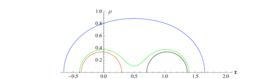
Figure 2: MOTS and Apparent Horizon for a system of two Black Holes

For systems of three black holes distributed in a symmetrical manner along the z axis, the critical separation is found by moving the outermost black holes farther away from the origin until no outermost MOTS is found.

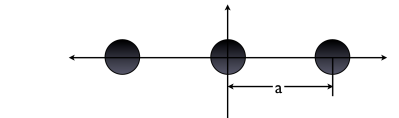
Figure 3: System of three Black Holes

In the case were the system has four black holes there are two distances that need to be taken into consideration. The distance between the inner black holes, defined here as $a$, and the distance between the outermost and inner black hole, defined here as $b$ (figure 4). In this case the critical values $a$ and $b$ are found by first finding the position of the outermost black holes that is farthest away from the origin ($f_{max}=a/2+b$) and then moving the inner black holes farther away until the largest value for $a$ is found with its corresponding value for $b$.

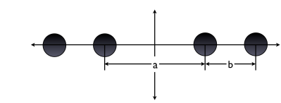
Figure 4: System of four Black Holes

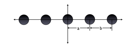
Figure 5: System of five Black Holes

The same method is used for a system of five black holes. The variable $a$ is now defined as the distance between the black hole located at the origin and either of the adjacent black holes, which are here referred to as inner black holes. The distance between the inner and outermost black hole is defined as $b$ (figure 5). Finding the critical separation is similar to the previous case of four black holes, but now $f_{max}=a+b$.

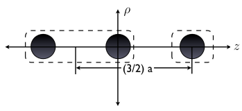
Figure 6: Three black holes represented as two black holes with a mass ratio of 2:1

For comparative reasons the black holes in each system are hypothetically grouped together in order to model the system as a two black hole system. This means that the black holes are assumed to be grouped in such a way that they would form two clusters. For example, in a system of three black holes we can put two black holes together and leave the third one by itself. This grouping results in a system of two black holes with a mass ratio of $2:1$ and a critical separation $a_{c}=1.5a$ (figure 6).

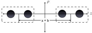
Figure 7: Four black holes represented as two black holes with a mass ratio of 1:1

The system of four black holes has two representations, one as a system of two black holes with a mass ratio $1:1$ and a critical separation equal to $a_{c}=a+b$ (figure 7), and a second one as a system of two black holes with a mass ratio of $3:1$ and a critical separation of $a_{c}=\frac{4a+8b}{6}$ (figure 8).

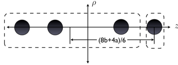
Figure 8: Four black holes represented as two black holes with mass ratio of 3:1

Finally the system of five black holes is represented as a system of two black holes with a mass ratio $3:2$ and a critical separation equal to $a_{c}=\frac{5}{6}(2a+b)$ (figure 9) and as a system with a mass ratio $4:1$ and a critical separation equal to $a_{c}=\frac{5}{4}(a+b)$ (figure 10).

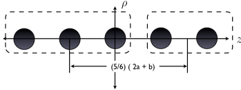
Figure 9: Five black holes represented as two black holes with a mass ratio of 3:2

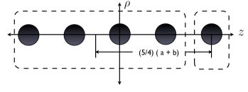
Figure 10: Five black holes represented as two black holes with a mass ratio of 4:1

2.4 Results

In the case of two black holes with different mass the method described in [23] was implemented to relate the mass ratio of the two black holes to the critical separation between them (table 1 and figure 11). The table was used to predict the critical separation for systems of $N$ black holes. To do this the systems of $N$ black holes was first represented as systems of two black holes. Then an equation for the critical separation was obtained in terms of $a$ and $b$ (see figures 6 7 8 9 and 10). Recall that depending on the representation used, each system has a specific mass ratio. Table 1 was used along with this ratio to find the critical separation that corresponds to each case. This value was then set equal to the equations for the critical separation and solved for $a$ and $b$.

Mass $M_{2}$	Critical Separation $a_{c}$	$a_{c}$ Normalized by total mass
1.0	1.531	0.7655
0.9	1.454	0.7653
0.8	1.375	0.7639
0.7	1.291	0.7594
0.6	1.208	0.7550
0.5	1.119	0.7460
0.4	1.026	0.7329
0.3	0.926	0.7123
0.2	0.816	0.6800
0.1	0.689	0.6264

Table 1: Two black holes of different mass ($M_{1}=1$ )

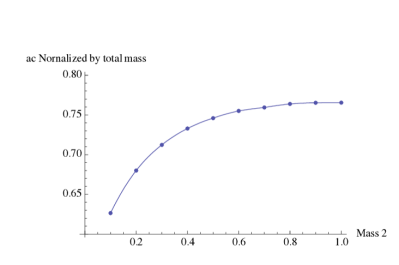
Figure 11: Plot of Critical separation normalized by mass vs. Mass of 2nd Black Hole

In the case of $N=3$ the mass ratio was $1:2$ and the critical separation normalized by mass was $\frac{a_{c}}{3}=\left(\frac{3a}{2}\right)\left(\frac{1}{3}\right)=0.746$ (see figure 6). Then:

$$\left(\frac{3a}{2}\right)\left(\frac{1}{3}\right) =0.7460\quad;\quad\quad a=1.492$$

In the case of $N=4$ we can create two equations:

$$\frac{a+b}{4}=0.7655\quad\textrm{ Mass ratio 1:1}$$

$$\frac{8b+4a}{24}=0.7203\quad\textrm{Mass ratio 1:3}$$

Solving for $a$ and $b$ gives $a=1.8022$ and $b=1.2598$. Finally in the case of $N=5$ we obtained:

$$\frac{2a+b}{6}=0.7582\quad\textrm{Mass ratio 2:3}$$

$$\frac{a+b}{4}=0.6982\quad\textrm{Mass ratio 1:4}$$

Solving for $a$ and $b$ gives $a=1.7564$ and $b=1.0364$.

The following table shows the results obtained for the critical separations $a$ and $b$ for systems of two, three, four and five black holes using the method described previously.

$N^{o}$ Black Holes	$a$	$b$
2	1.531	–
3	1.528	–
4	1.340	1.609
5	1.370	1.650

Table 2: Critical Separations $a$ and $b$ for two, three, four and five black holes

Comparing these results to the ones predicted by table 1 gives the following errors:

$N^{o}$ Black Holes	Numerical $a$	Predicted $a$	Error	Numerical $b$	Predicted $b$	Error
3	1.528	1.492	2.36%	–	–	–
4	1.340	1.802	34.49%	1.609	1.260	21.70%
5	1.370	1.756	28.20%	1.650	1.036	37.19 %

Table 3: Critical separations: Comparison between numerical results and predicted results

Were:

$$\textrm{Error}=\frac{100}{\textrm{Numerical}\quad a}(|\textrm{Numerical}\quad a-\textrm{Predicted}\quad a|)$$

2.5 Discussion

Note that these values are close to the ones predicted by table 1 and can provide a good first guess for finding the critical separations of systems of $N$ black holes. Although the percentage error might seem large, when presented with the situation of making a preliminary estimate for the values for these critical separations in a system of $N$ black holes, which is useful information when determining the location of the apparent horizon, any estimate that is 20% or 30% of the actual value is reasonable.

This method can be extended to predict the location of the apparent horizon for a system of any $N$ black holes symmetrically distributed by following the these steps:

• Count the number of critical separations $a_{i}$. If $N$ is odd then the number of critical separations, $M$, is $\frac{N-1}{2}$ and if $N$ is even then the number of critical separations is $\frac{N}{2}$.

• Establish all the possible distinct groupings of the $N$ black holes that would simulate a system of two black holes. The number of groupings should be equal to the number of critical separations $M$.

• For each grouping determine the location of the center of mass for the two clusters. Let $r_{1}$ ($r_{2}$) be the distance between the axis of symmetry and the center of mass of the left cluster (right cluster).

• For each grouping find the mass ratio of the two clusters and using table 1 interpolate the critical separation $a_{c}$ that corresponds to that mass ratio.

• Solve the system of equations given by $r_{1}+r_{2}=a_{c}$ to find the values of all critical separations $a_{1}\cdots a_{M}$.

By analyzing a system of two black holes we have been able to predict the critical separations for system of multiple black holes. We have developed a method that provides an adequate first approximation of these critical separations and that if applied can significantly reduce the time needed to find the apparent horizon by telling us if we should be looking for a common apparent horizon that engulfs all black holes, or if we should be looking for individual apparent horizons surrounding each body.

3 Black hole with a ring singularity

The Motivation for studying black hole rings comes from computational results from Shapiro et. al. [29] in which the collapse of a rotating toroidal configuration of collsionless particles to Kerr black holes gives rise initially to an event horizon with toroidal topology. The event horizon eventually becomes topologically spherical. In this paper they explain that there is no violation of topological censorship since when the toroidal horizon forms the points in the inner rim of the torus (the whole of the torus) are spacelike. This implies that the hole closes up faster than the speed of light.

Their analysis begins with a two dimensional surface which has the topology of an oblate spheroid. This surface will eventually represent the event horizon after the black hole has reached its equilibrium state. They trace back the light rays emanating in the normal direction inward to the surface. The boundary of the spacetime points in the casual past of this surface will be generated by the set of light rays emanating from the surface that cross other light rays or that focus to a point (that form a caustic). They further explain that in this case, where the initial surface is an oblate spheroid, the rays that focus to a point will cross other light rays before they form a caustic. So in essence the boundary of the casual past of this surface is represented by the spacelike surface where all rays cross (the crossover surface $X$). They have shown that this surface X has toroidal topology.

They further explain that once the black hole has reached its equilibrium state and the event horizon has its full complement of generators then this horizon will have spherical topology (namely the oblate spheroid represented by the above mentioned surface) agreeing with theorems developed by Galloway and Browdy [30, 18].

What we want to do here is to use the apparent horizon as an approximation to the event horizon. We will apply the previous method used for finding the apparent horizon for systems of $N$ black holes to the case of a black hole ring. This will allow us to find a specific mass of the black hole ring that allows the formation of such toroidal event horizon.

3.1 Equations

To adapt the equations developed by Bishop [22] and used in Sec. 2, we first need to develop a new conformal factor that takes into account the new circular shape of the black hole. To do so recall that the conformal factor is given by:

$$\Psi=1+\sum_{i}\frac{m_{i}}{2R_{i}}$$ (31)

Where $R_{i}=r-r_{i}$ is the difference between a reference point $r=(\rho,z)$ and the location of the $i^{th}$ black hole $r_{i}=(\rho_{i},z_{i})$.

Consider a ring in the $z=0$ plane of radius $\rho=\rho_{o}$, then the distance in cylindrical coordinates between any point in space ($\rho,\varphi,z$) and the ring is given by S:

$$S^{2}=z^{2}+(\rho\cos{\varphi}-\rho_{o}\cos{\theta})^{2}+(\rho\sin{\varphi}-\rho_{o}\sin{\theta})^{2}$$ (32)

Simplifying this expression we get:

$$S^{2}=z^{2}+\rho^{2}+\rho_{o}^{2}-2\rho\rho_{o}\cos{(\theta-\varphi)}$$ (33)

Then the conformal factor for the metric is given by:

$$\Psi=1+\int_{0}^{2\pi}\frac{M}{2\,S}d\phi\;,\quad\phi=\theta-\varphi$$ (34)

Here $M$ is the mass of the black hole ring.

Note that if the following conditions hold:

$$Re[z^{2}+(\rho-\rho_{o})^{2}]>0$$

$$Re[z^{2}+(\rho+\rho_{o})^{2}]>0$$

$$\left|Re\left[\frac{z^{2}+\rho^{2}+\rho_{o}^{2}}{\rho\rho_{o}}\right]\right|\geq 2 \frac{z^{2}+\rho^{2}+\rho_{o}^{2}}{\rho\rho_{o}}\in\mathds{C}$$ or (35)

then:

$$\Psi=1+\frac{M}{2}\left[\frac{2\textrm{EllipticK}[\frac{-4\rho\rho_{o}}{z^{2}+(\rho-\rho_{o})^{2}}]}{\sqrt{z^{2}+(\rho-\rho_{o})^{2}}}+\frac{2\textrm{EllipticK}[\frac{4\rho\rho_{o}}{z^{2}+(\rho+\rho_{o})^{2}}]}{\sqrt{z^{2}+(\rho+\rho_{o})^{2}}}\right]\\$$ (36)

In Mathematica the EllipticK function is defined in such a way that its Taylor expansion around $x=0$ gives:

$$\frac{\pi}{2}+\frac{\pi x}{8}+\frac{9\pi x^{2}}{128}+\frac{25\pi x^{3}}{512}+\frac{1225\pi x^{4}}{32768}+\frac{3969\pi x^{5}}{131072}+\frac{53361\pi x^{6}}{2097152}+\frac{184041\pi x^{7}}{8388608}+O[x]^{8}$$

On the other hand if:

$$Im\left[\frac{z^{2}+\rho^{2}+\rho_{o}^{2}}{\rho\rho_{o}}\right]=0\quad \quad\left|Re\left[\frac{z^{2}+\rho^{2}+\rho_{o}^{2}}{\rho\rho_{o}}\right]\right|<2$$ and

$$\textrm{or}\quad Re\left[z^{2}+(\rho-\rho_{o})^{2}\right] \leq 0$$

$$\textrm{or}\quad Re\left[z^{2}+(\rho+\rho_{o})^{2}\right] \leq 0$$ (37)

then the integral in equation 34 can be performed. However, these last conditions will never hold since $z,\rho$ and $\rho_{o}$ are real numbers. A plot of the function:

$$f=\frac{z^{2}+\rho^{2}+\rho_{o}^{2}}{\rho\rho_{o}}$$ (38)

rewritten using $Z=\frac{z}{\rho}$ and $p=\frac{\rho_{o}}{\rho}$

$$f=\frac{Z^{2}+p^{2}+1}{p}$$ (39)

Shows that the expression $\left|Re\left[\frac{z^{2}+\rho^{2}+\rho_{o}^{2}}{\rho\rho_{o}}\right]\right|<2$ will never hold:

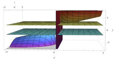
Figure 12: Plot to show $\left|Re\left[\frac{z^{2}+\rho^{2}+\rho_{o}^{2}}{\rho\rho_{o}}\right]\right|\not<2$

Hence the conformal factor $\Psi$ should be represented as in equation 36. Used in conjunction with Bishop’s equations LABEL:Bishopeq we are able to find apparent horizons for black hole rings.

3.2 Procedures

To find the apparent horizon, we again use equations 28 and we start with the following initial conditions:

$$A(0)=\rho_{o},\quad B(0)=0,\quad\alpha(0)=0$$ (40)

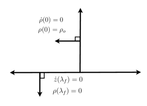
Figure 13: First set of boundary conditions for a black hole ring

These initial conditions represent rays leaving perpendicular to the $\rho$-axis ( $\dot{\rho}(0)=0$) at the location $\rho(0)=\rho_{o}$. We are interested in the rays that arrive perpendicular to the $z$-axis since these rays will fulfill the boundary condition $\dot{z}(\lambda_{f})=0$ (where $\lambda_{f}$ represents the value of the parameter $\lambda$ when the ray returns to the $z$-axis) and therefore they will represent the marginally outer trapped surface. Unfortunately choosing to work in cylindrical coordinates to account for the cylindrical symmetry does not allow these rays to cross the $z$-axis and consequently we are not able to use of the Bisection method to locate them accurately. We therefore choose to use a visual method to find them. Since rays that are in the marginally outer trapped surface never leave the surface, this means that these rays will retrace their steps if the numerical integration code is left to run for a long enough time. Hence we identify the apparent horizon with these rays.

Once this first approximation is obtained a new integration is performed, this time using the same boundary conditions that we used for finding the marginally trapped surfaces in the case of a system of $N$ black holes:

$$A(0)=0,\quad B(0)=0,\quad C(0)=0$$ (41)

Which need the same Taylor expansion as before, to avoid division by zero:

$$A(0)=2\lambda_{o},\quad B(0)=2\lambda_{o}z_{0},\quad C(0)=\pi\lambda_{o}$$ (42)

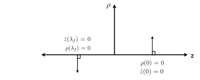
Figure 14: Second set of boundary conditions for a black hole ring

The point $z(\lambda_{f})$ in our first approximation, where the ray reaches the $z$-axis perpendicularly, is going to be the starting point for our second approximation. Now we can use the Bisection method to find the apparent horizon. This means that we are looking for rays that fulfill $\dot{\rho}=0$ at $z=0$.

3.3 Results

We present the some of the results obtained for the location of the apparent horizon of a ring singularity of radius 1 in figure 16, the rest are presented in appendix A. The graphs show that as the mass decreases the apparent horizon becomes compressed along the $z$-axis, consistent with the results observed in the paper [29], where they find a final event horizon with the topology of an oblate spheroid. This results are better represented in table 4, which shows the values obtained for the minor radius of the apparent horizons $C_{1}$, their major radius $C_{2}$ and the ratio $C_{1}/C_{2}$.

Mass $M$	$C_{1}$	$C_{2}$	$C_{1}/C_{2}$
1.0$\pi$	6.226	6.311	0.987
0.8$\pi$	4.955	5.062	0.979
0.6$\pi$	3.674	3.816	0.9623
0.5$\pi$	3.026	3.197	0.946
0.4$\pi$	2.367	2.581	0.917
0.3$\pi$	1.683	1.972	0.853
0.25$\pi$	1.320	1.670	0.790
0.2$\pi$	0.917	1.369	0.670
0.19$\pi$	0.825	1.307	0.631
0.18$\pi$	0.724	1.243	0.582
0.17$\pi$	0.604	1.174	0.514
0.165$\pi$	0.523	1.132	0.462
0.163$\pi$	0.478	1.110	0.430

Table 4: Results used for Extrapolation (Radius of black hole ring is 1)

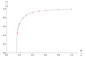
Figure 15: Plot of axis ratio $C_{1}/C_{2}$ as a function of mass $M/\pi$

This table allowed us to establish a relation between the ratio $C_{1}/C_{2}$ and the mass of the black hole ring. A plot of $C_{1}/C_{2}$ versus mass $M/\pi$ is shown in figure 15. Note how sharply the ratio decreases once the mass of the black hole ring is less than $M=0.2\pi$. Using the interpolation function from Mathematica we found that the mass that returns a ratio $C_{1}/C_{2}=0$ is $M=0.15\pi$. Since there is an inverse relation between the mass and radius of the ring, we can thus predict a critical radius that will produce a toroidal event horizon using the value we obtained for the mass. That is the critical radius is $R=1/(0.15\pi)=20/(3\pi)$.

Figure 16: Apparent Horizon for ring masses $m=0.17,0.18,0.19,0.20$ of radius 1

3.4 Discussion

The main goal of this section was to develop a method for predicting the size of a black hole ring that would give rise to an event horizon of toroidal topology. This was accomplished by deducing the conformal factor for a black hole ring and adapting the apparent horizon equations found in [22] [23] accordingly. The key argument here is that even though an apparent horizon can never have toroidal topology we can still use it to approximate the event horizon of black hole rings that have spherical topology. The apparent horizon will follow the shape of the event horizon up until it eventually becomes toroidal. So the information we gathered for the flattening of the apparent horizon can then be used to extrapolate the value of the ring’s mass that would give rise to a toroidal event horizon. The results suggest that when the ring singularity has a mass of $M=1$ and a radius $R=20/(3\pi)\approx 2.12$ (or equivalently when the ring has a mass of $M=0.15\pi$ and a radius of $R=1$) the event horizon would have toroidal topology.

4 Conclusion

As mentioned in the introduction apparent horizons are important in numerical relativity because they provide a quasilocal boundary for the black hole region. For instance, they are used in numerical simulations to locate the black holes so that black hole excision techniques can be used. They also provide physical information about the black holes such as mass and angular momentum. With this in mind and considering that recent full numerical research has focused on systems of three black holes, we have focused our attention on gaining a better understanding of systems of $N$ black holes.

To begin this analysis we focused on a time-symmetric spacelike hypersurface with the purpose of developing a method for finding the critical separations between the black holes in the system. This was done by first analyzing a system of two black holes with different mass and finding the critical separation for each mass ratio. The result was a table that was used to predict the critical separations for systems of $N$ black holes, represented as a system of two black holes. This proved to be a good method for finding a first guess of these critical separations. The errors obtained when comparing the actual critical separation to the one predicted by the table were around 20% to 40%. Although at first glance this errors seem large, when confronted with a system of $N$ black holes, knowing whether to look for a common apparent horizon or individual apparent horizons makes a big difference on computational time.

Our next step was to consider a black hole ring. This was motivated by papers which suggested the existence of event horizons of toroidal topology in rotating clusters with toroidal topology. The equations used to find the apparent horizon for the system of $N$ black holes were adapted using a conformal factor that takes into account the circular shape of the ring singularity. We vary its mass, while keeping its radius constant, and computed its apparent horizon. The results were apparent horizons with the topology of an oblate spheroid. A certain minimal mass was attained that did not allowed the formation of any spherical apparent horizon suggesting that there is either no horizon or the actual shape might be toroidal and therefore not predictable by the algorithm. Using the data obtained we constructed a table that relates the mass of the black hole ring to the ratio of the minor radius to major radius of the apparent horizon. Using this information we extrapolated the mass that corresponds to a radius ratio equal to zero, thus suggesting that this critical mass will correspond to a black hole ring with a toroidal event horizon. Since there is an inverse relation between the mass and radius of the ring we can alternatively, for a fixed mass of 1, find the critical radius of the ring which in this case is $20/(3\pi)\approx 2.12$ M. While due to the smoothness of the apparent horizon surfaces we cannot see a toroidal surface, it is interesting to study the event horizon evolution for this configuration [17].

A different way of constructing a toroidal horizon would be to consider a set of $N$ black holes distributed along a circle at a critical separation that connects all nearby horizons together. If one succeeds to do this on a circle of radius 2.12 at least, with a total mass of 1, according to the previous discussion we could create a toroidal horizon. In order to evaluate this possibility with the apparent horizon information we have obtained in Table 2 we can study the progression of the critical length per mass covered by a line distribution of $N$ black holes, representing an approximation to an small portion of a ring.

Two black holes separated at a critical length $a_{c}$ will cover a length

$$\ell_{c}/M=(a_{c}/2+a_{c}+a_{c}/2)/N=2\,a_{c}/2=1.531.$$

For three black holes, see Fig. 3

$$\ell_{c}/M=(a_{c}/2+2\,a_{c}+a_{c}/2)/N=3\,a_{c}/3=1.528.$$

For four black holes, see Fig. 4

$$\ell_{c}/M=(b_{c}/2+b_{c}+a_{c}+b_{c}+b_{c}/2)/N=(a_{c}+3\,b_{c})/4=1.54175.$$

And for five black holes, see Fig. 5

$$\ell_{c}/M=(b_{c}/2+b_{c}+2\,a_{c}+b_{c}+b_{c}/2)/N=(2\,a_{c}+3\,b_{c})/5=1.538.$$

So, essentially we cover 1.54 of a circle perimeter of unit mass, but we would need to cover a perimeter of $2.12\times 2\pi=13.32$. This leaves us with a deficit factor of 8.65 to realize the toroidal horizon with this construction. However, since event horizons can show some fine structure at the moment of merging, it is worth studying this configuration in a more dynamical setting [17].

In our search of common apparent horizons for rings of increasing radius in Sec. 3 we have not been able to find any beyond $R=2.12$. See Fig. 15. This leads to the question of the nature of the object left exposed without a dressing horizon. We recall the form of the conformal factor of the 3-metric

$$\Psi=1+2M\left[\frac{\textrm{EllipticK}\left(\sqrt{\frac{2\rho\rho_{0}}{z^{2}+(\rho+\rho_{o})^{2}}}\right)}{\sqrt{z^{2}+(\rho+\rho_{o})^{2}}}\right]$$ (43)

Where this EllipticK function near the ring behaves like [31, page 591],

$$\textrm{EllipticK}(\sqrt{x})\to\frac{1}{2}\ln\left(\frac{16}{1-x}\right),$$ (44)

for $x\to 1$. This limit corresponds to approaching the ring as $\rho\to\rho_{0}$ and $z\to 0$. Upon double differentiation of the metric to compute the curvature components, we find terms that diverge like $\ln^{3}|1-x|/|1-x|^{2}$. One can show that those effectively are true singularities of the spacetime computing, for instance, scalar invariants [17].

Acknowledgments:
The authors acknowledge important discussions with M.Campanelli, B.Krishnan, M.Ponce, and Y.Zlochower. We gratefully acknowledge the NSF for financial support from Grants No. PHY-0722315, No. PHY-0653303, No. PHY-0714388, No. PHY-0722703, No. DMS-0820923, and No. PHY-0929114; and NASA for financial support from NASA Grants No. 07-ATFP07-0158 and No. HST-AR-11763. Computational resources were provided by the Ranger cluster at TACC (Teragrid allocation TG-PHY060027N) and by NewHorizons at RIT.

Appendix A: Apparent horizons for black hole rings

The following are the results obtained when finding the apparent horizon for a ring singularity.

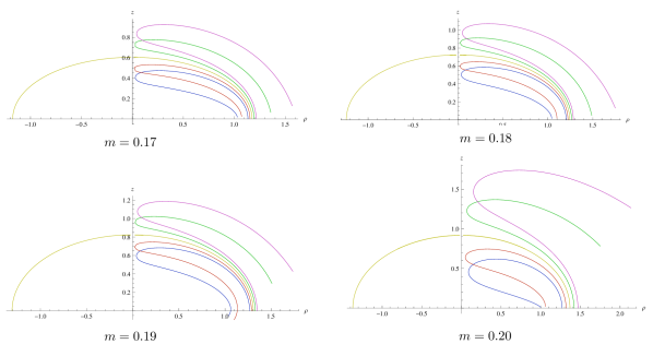
Figure 17: Apparent Horizon for a ring of radius 1 and masses $m=0.17,0.18,0.19,0.20$

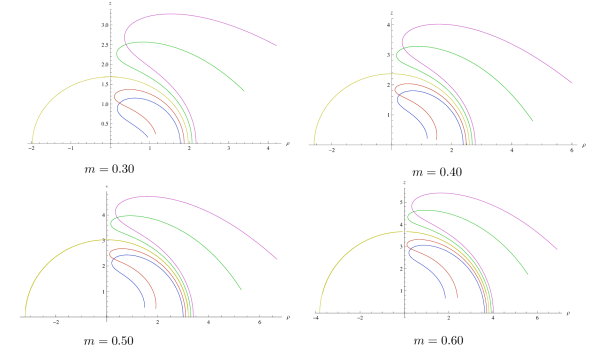
Figure 18: Apparent Horizon for a ring of radius 1 and masses $m=0.30,0.40,0.50,0.60$

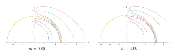
Figure 19: Apparent Horizon for a ring of radius 1 and masses $m=0.80,1.00$

Appendix B: Data for systems of four and five black holes

The first set of data was obtained when finding the apparent horizon for four symmetrically distributed black holes. The distance $a$ represents the distance between the two inner black holes. The distance $b$ represents the distance between the outer black holes and the inner black holes. The second set of data was obtained when finding the apparent horizon for five symmetrically distributed black holes. The value $a$ represents the distance between the middle black hole and the inner black holes. The distance $b$ represents the distance between the outer black holes and the inner black holes.

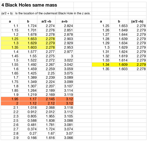
Figure 20: Data obtained for a system of 4 black holes

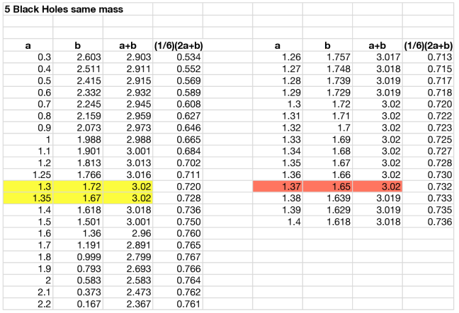
Figure 21: Data obtained for a system of 5 black holes

Appendix C: Code used for finding apparent horizons

For a detailed description of the NDSolve command from Mathematica, which was used to solve the system of non linear ODE’s, please refer to :

http://reference.wolfram.com/mathematica/ref/NDSolve.html

The method used for the integration was an extrapolation method. This method was chosen because, as explained in the Mathematica documentation, it is an arbitrary order method that has automatic order and step size controls. The arbitrary order means that they can be arbitrarily faster than fixed-order methods for very precise tolerances. A more detailed description of extrapolation methods can be found in [32]. The sub-method used is a linearly implicit Euler method (Also known as backward Euler method). For more information the following website contains a complete description of the extrapolation method.

http://reference.wolfram.com/mathematica/tutorial/NDSolveExtrapolation.html

References

References

- [1] Frans Pretorius. Evolution of binary black hole spacetimes. Phys. Rev. Lett., 95:121101, 2005.
- [2] Manuela Campanelli, C. O. Lousto, P. Marronetti, and Y. Zlochower. Accurate evolutions of orbiting black-hole binaries without excision. Phys. Rev. Lett., 96:111101, 2006.
- [3] John G. Baker, Joan Centrella, Dae-Il Choi, Michael Koppitz, and James van Meter. Gravitational wave extraction from an inspiraling configuration of merging black holes. Phys. Rev. Lett., 96:111102, 2006.
- [4] Manuela Campanelli, Carlos O. Lousto, Yosef Zlochower, and David Merritt. Large merger recoils and spin flips from generic black-hole binaries. Astrophys. J., 659:L5–L8, 2007.
- [5] Manuela Campanelli, Carlos O. Lousto, Yosef Zlochower, and David Merritt. Maximum gravitational recoil. Phys. Rev. Lett., 98:231102, 2007.
- [6] Sergio Dain, Carlos O. Lousto, and Yosef Zlochower. Extra-Large Remnant Recoil Velocities and Spins from Near- Extremal-Bowen-York-Spin Black-Hole Binaries. Phys. Rev. D, 78:024039, 2008.
- [7] Geoffrey Lovelace, Robert Owen, Harald P. Pfeiffer, and Tony Chu. Binary-black-hole initial data with nearly-extremal spins. Phys. Rev., D78:084017, 2008.
- [8] Mark Hannam, Sascha Husa, Denis Pollney, Bernd Brugmann, and Niall O’Murchadha. Geometry and Regularity of Moving Punctures. Phys. Rev. Lett., 99:241102, 2007.
- [9] J. David Brown. Probing the puncture for black hole simulations. Phys. Rev., D80:084042, 2009.
- [10] Jason D. Immerman and Thomas W. Baumgarte. Trumpet-puncture initial data for black holes. Phys. Rev., D80:061501, 2009.
- [11] Mark Hannam, Sascha Husa, and Niall O Murchadha. Bowen-York trumpet data and black-hole simulations. Phys. Rev., D80:124007, 2009.
- [12] Manuela Campanelli, Carlos O. Lousto, and Yosef Zlochower. Algebraic Classification of Numerical Spacetimes and Black-Hole-Binary Remnants. Phys. Rev. D, 79:084012, 2009.
- [13] Manuela Campanelli, C. O. Lousto, and Y. Zlochower. Spinning-black-hole binaries: The orbital hang up. Phys. Rev. D, 74:041501(R), 2006.
- [14] Manuela Campanelli, Carlos O. Lousto, Yosef Zlochower, Badri Krishnan, and David Merritt. Spin flips and precession in black-hole-binary mergers. Phys. Rev., D75:064030, 2007.
- [15] Olaf Dreyer, Badri Krishnan, Deirdre Shoemaker, and Erik Schnetter. Introduction to isolated horizons in numerical relativity. Phys. Rev., D67:024018, 2003.
- [16] Badri Krishnan, Carlos O. Lousto, and Yosef Zlochower. Quasi-Local Linear Momentum in Black-Hole Binaries. Phys. Rev., D76:081501, 2007.
- [17] Y.Zlochower M.Ponce, C.O.Lousto. Toroidal event horizons from initially stationary bh configurations. 2010. in preparation.
- [18] Gregory J. Galloway. Rigidity of outer horizons and the topology of black holes. 2006.
- [19] Jonathan Thornburg. Event and Apparent Horizon Finders for Numerical Relativity. Living Rev. Rel., 10:3, 2007.
- [20] M. Alcubierre. Introduction to 3+1 Numerical Relativity. Oxford University Press, 2008.
- [21] Ivan Booth. Black hole boundaries. Can. J. Phys., 83:1073–1099, 2005.
- [22] N. T. Bishop. The closed trapped region and the apparent horizon of two Schwarzschild black holes. Gen. Rel. Grav., 14(9):717–723, 1982.
- [23] N. T. Bishop. The horizons of two Schwarzschild black holes. Gen. Rel. Grav., 16(6):589–593, 1984.
- [24] Manuela Campanelli, Miranda Dettwyler, Mark Hannam, and Carlos O. Lousto. Relativistic three-body effects in black hole coalescence. Phys. Rev., D74:087503, 2006.
- [25] Manuela Campanelli, Carlos O. Lousto, and Yosef Zlochower. Close encounters of three black holes. Phys. Rev. D, 77:101501(R), 2008.
- [26] Carlos O. Lousto and Hiroyuki Nakano. Three-body equations of motion in successive post-newtonian approximations. Class. Quant. Grav., 25:195019, 2008.
- [27] Carlos O. Lousto and Yosef Zlochower. Foundations of multiple black hole evolutions. Phys. Rev., D77:024034, 2008.
- [28] Kayhan Gultekin, M. Coleman Miller, and Douglas P. Hamilton. Three-body encounters of black holes in globular clusters. AIP Conf. Proc., 686:135–140, 2003.
- [29] S. Shapiro, S. Teukolsky, and Jeffrey Winicour. Toroidal black holes and topological censorship. Phys. Rev. D, 52(12):6982–6987, 1995.
- [30] S. F. Browdy and G. J. Galloway. Topological censorship and the topology of black holes. J. Math. Phys., 36:4952–4961, 1995.
- [31] Milton Abramowitz and Irene Stegun. Handbook of Mathematical Functions. Dover, New York, 10th edition, 1972.
- [32] J. Stoer and R. Bulirsch. Introduction to Numerical Analysis. Springer-Verlag, Berlin and New York, 1980.