Kondo effects in a triangular triple quantum dot with lower symmetries

Abstract

We study the low-energy properties and characteristic Kondo energy scale of a triangular triple quantum dot, connected to two non-interacting leads, in a wide parameter range of a gate voltage and distortions which lower the symmetry of an equilateral structure, using the numerical renormalization group approach. For large Coulomb interactions, the ground states with different characters can be classified according to the plateaus of $\Theta\equiv(\delta_{\mathrm{e}}-\delta_{\mathrm{o}})(2/\pi)$, where $\delta_{\mathrm{e}}$ and $\delta_{\mathrm{o}}$ are the phase shifts for the even and odd partial waves. At these plateaus of $\Theta$, both $\Theta$ and the occupation number $N_{\mathrm{tot}}\equiv(\delta_{\mathrm{e}}+\delta_{\mathrm{o}})(2/\pi)$ take values close to integers, and thus the ground states can be characterized by these two integers. The Kondo effect with a local moment with total spin $S=1$ due to a Nagaoka mechanism appears on the plateau, which can be identified by $\Theta\simeq 2.0$ and $N_{\mathrm{tot}}\simeq 4.0$. For large distortions, however, the high-spin moment disappears through a singlet-triplet transition occurring within the four-electron region. It happens at a crossover to the adjacent plateaus for $\Theta\simeq 0.0$ and $\Theta\simeq 4.0$, and the two-terminal conductance has a peak in the transient regions. For weak distortions, the SU(4) Kondo effect also takes place for $N_{\mathrm{tot}}\simeq 3.0$. It appears as a sharp conductance valley between the $S=1/2$ Kondo ridges on both sides. We also find that the characteristic energy scale $T^{*}$ reflect these varieties of the Kondo effect. Particularly, $T^{*}$ is sensitive to the distribution of the charge and spin in the triangular triple dot.

I Introduction

The triangle is the simplest polygon, and has a closed loop which plays an important role on various fascinating phenomena in the condensed matter physics. The closed path in a metal and semiconductor allows the electrons to move around the loop, and causes a quantum-mechanical interference effects, such as an Aharanov-Bohm (AB) effect.AB ; Webb The closed path consisting of the odd-number of links also causes frustration, which leads to resonating valence bonds for some anti-ferromagnetic systems.RVB

Furthermore, the interplay between the strong correlation and the interference effects caused by the triangular structure has also been one of the topics of the current interests in different fields of the condensed matter physics. For instance, the single triangle is also a fundamental unit of the triangular and kagomé lattices. In these systems the geometrical frustration affects significantly the magnetic properties and the behavior at the Mott-Hubbard metal-insulator transition.Koshibae1 ; Furukawa_Kawakami Another interesting example is the triangular trimer of Cr atoms placed upon an Au surface,Jamneala ; Affleck3a ; Zarand and this system is expected to show a non-Fermi-liquid behavior due to the multi-channel Kondo effect.NozieresBlandin ; CoxZawadowski

Recently, the triangular triple quantum dot (TTQD) has been experimentally realized and intensively studied using various systems, such as AlGaAs/GaAs heterostructuresVidan-Stopa ; Canada ; Amaha2 ; Amaha3 ; RoggeHaug and self-assembled InAs quantum dot.Amaha1 Theoretically, the TTQD has been shown to demonstrate various types of the Kondo effects, ONTN ; Numata ; Numata2 ; Zitko2 ; Logan3 ; Ulloa as well as the AB effect.KKA1 ; DelgadoShimKorkusinskiHawrylak The closed path makes the TTQD different from a linear quantum-dot chainao99 ; aoQuasi ; OH ; ONH ; NO ; KKA2 ; Zitko ; Zitko_Bonca and the other three-level systems. Eto ; Sakano ; LeoFabrizio ; Kita ; Hecht_3 ; Paaske One of the most interesting points is that the appearance of a local moment with total spin $S=1$, at the filling where one additional electron is introduced into half-filling.ONTN ; KorkusinskiGimenezHawrylakETAL This is caused by a Nagaoka ferromagnetic mechanism for the electrons moving around the triangular structure. Nagaoka The $S=1$ moment shows a Kondo behavior when the leads are coupled to the quantum dots.ONTN ; Numata ; Numata2 Another interesting point is that the SU(4) Kondo effect takes place at half-filling, ONTN ; Numata ; Numata2 ; Logan3 ; Zitko2 ; Ulloa in the case where the ground state has a 4-fold degeneracy caused by the orbital and spin degrees of freedoms. The TTQD has provided a new variety to the SU(4) Kondo effect, which had been studied for the double-dot systems. Borda ; Logan_2dotA ; Mravlje_Ramsak_Rejec ; Anders_Logan

The number of leads connected to the TTQD also affects significantly the Kondo behavior. This is because whether or not the local moment can be screened depends on the relation between the dimension of the Hilbert space for the local moment and the number of conducting channels.NozieresBlandin The low-temperature properties of the TTQD have been studied, so far, by several theoretical groups, for the configurations with one,Logan3 two,ONTN ; Numata ; Numata2 ; Zitko2 ; Ulloa and three leads.Ulloa These studies complement each other the wide parameter space of the TTQD. Žitko et alZitko2 and Mitchell et alLogan3 studied the Kondo effect at half-filling in some situations, but the dependence on the electron filling was not examined. Vernek et al Ulloa examined the gate voltage $\epsilon_{d}$ dependence in a wide range of the electron filling, but the parameters used were confined to a region of small interaction $U$ and a large dot-lead coupling $\Gamma$ where the Kondo behavior is still rather smeared.

We have studied the Kondo behavior of the TTQD away from half-filling in the series of the works.ONTN ; Numata ; Numata2 Our research in the early stageONTN started with a theoretical observation of a two-stage Kondo screening of the $S=1$ Nagaoka high-spin at four-electron filling and a sharp conductance dip caused by the SU(4) Kondo effect at half-filling (with three electrons), appearing in the gate-voltage dependence. The precise features of these Kondo effects have been clarified further in the previous paper,Numata2 for the parameter values which cover the weak and strong couplings with respect to both $U$ and $\Gamma$. We have also examined the effects of the perturbations which break the full symmetry of the equilateral triangle,Numata2 as the real TTQD systems have some deviations from the regular structure in most of cases. Our results, obtained with the Wilson numerical renormalization group (NRG),KWW ; KWW2 have shown that the conductance dip typical of the SU(4) Kondo effect in the TTQD is quite sensitive to the perturbation, while the $S=1$ Kondo behavior is robust.Numata2

The distortions of the triangular structure discussed in the previous paper, however, were still relatively small, so that the overall features of the Kondo effect in the TTQD have not yet been fully revealed and much remains to be explored. Particularly, a singlet-triplet transition between a local singlet and the Nagaoka high-spin state occurs in the isolated TTQD cluster for large deformations, and this transition will affect the Kondo behavior at four-electron filling. Furthermore, the behavior of the conductance dip due to the SU(4) Kondo effect also needs to be clarified in more detail.

The purpose of the present work is to provide a comprehensive overview of the Kondo effect in the TTQD and to study the effects of large distortions. Specifically, we examine two different types of distortion: ($i$) an irregular inter-dot coupling, and ($ii$) an inhomogeneity in the level position of the quantum dots. We calculate the phase shifts, $\delta_{\mathrm{e}}$ and $\delta_{\mathrm{o}}$, for the even and odd partial waves of the renormalized quasi-particles, in a wide parameter region of the gate voltage $\epsilon_{d}$ and the distortions. These two phase shifts determine the ground state properties of the TTQD connected to two leads.

In the parameter space for large $U$ and small $\Gamma$, we find plateau with the integer values of the phase difference $\Theta\equiv(\delta_{\mathrm{e}}-\delta_{\mathrm{o}})(2/\pi)$, and at each plateau the occupation number given by the Friedel sum rule $N_{\mathrm{tot}}\equiv(\delta_{\mathrm{e}}+\delta_{\mathrm{o}})(2/\pi)$ also approaches to an integer. These plateaus, therefore, can be classified with the two integer set $(N_{\mathrm{tot}},\,\Theta)$, and each plateau corresponds to the ground state realized in each parameter region. For instance, the plateau for the $S=1$ Kondo region can be labelled as $(N_{\mathrm{tot}},\,\Theta)\simeq(4.0,\,2.0)$. The singlet-triplet transition emerges as a steep rise in $\Theta$ to the adjacent plateaus with the label $(N_{\mathrm{tot}},\,\Theta)\simeq(4.0,\,0.0)$ and $(4.0,\,4.0)$, situated in the regions of a large distortion. Therefore, the two-terminal conductance $g_{\mathrm{s}}$ shows a peak of the unitary-limit value $g_{\mathrm{s}}=2e^{2}/h$ in the middle of the rise. We also find that the SU(4) Kondo behavior appears in the parameter space along the contour line for $\Theta=2.0$, which traverses the middle of the steep rise in $\Theta$ between the plateaus with $\Theta\simeq 1.0$ and $\Theta\simeq 3.0$, for $N_{\mathrm{tot}}\simeq 3.0$.

We also estimate the characteristic energy scale $T^{*}$ of the Kondo screening in the wide parameter region, from the flow of the low-lying excitation energies in the NRG. The energy scale $T^{*}$ depends strongly on the local charge distribution in the TTQD. The screening is protracted significantly in the case where the partial component of the local moment becomes large at the apex site, which is located away from the leads as shown in Fig. 1 (a). This is because that the tunneling processes of the conduction electrons from the leads to the apex site tend to be suppressed in the intermediate states on the other two sites.

The paper is organized as follows. We describe the model and the formulation in Sec. II. Some characteristics of the TTQD, seen already in the non-interacting case of $U=0$, are summarized in Sec. III. Then, the molecular limit $\Gamma\to 0$ for finite $U$ is considered in Sec. IV in order to see the basic features of the local charge and spin states of the TTQD. The NRG results for the ground-state properties are shown in Sec. V. The results for the characteristic energy scale $T^{*}$ are presented in Sec. VI. A summary is given in Sec. VII.

Figure 1: Triangular triple quantum dot in (a) series and (b) parallel configurations. The dot which has no direct connection to the leads is referred to as the apex site, and labeled as $i=2$ in the text.

II Formulation

II.1 TTQD connected to two non-interacting leads

We consider a three-site Hubbard model on a triangular cluster as a model for the TTQD. The cluster is connected to two non-interacting leads on the left ($L$) and right ($R$) as illustrated in Fig. 1 (a). The Hamiltonian is given by

$$\mathcal{H}=\mathcal{H}_{\mathrm{dot}}^{0}+\mathcal{H}_{\mathrm{dot}}^{U}+\mathcal{H}_{\mathrm{mix}}+\mathcal{H}_{\mathrm{lead}}\;,$$ (1)

$$\mathcal{H}_{\mathrm{dot}}^{0}=\,-\sum_{<ij>}^{N_{D}}\sum_{\sigma}t_{ij}\left(d^{\dagger}_{i\sigma}d^{\phantom{\dagger}}_{j\sigma}+d^{\dagger}_{j\sigma}d^{\phantom{\dagger}}_{i\sigma}\right)$$

$$\qquad\quad\ +\sum_{i=1}^{N_{D}}\sum_{\sigma}\epsilon_{d,i}\,d^{\dagger}_{i\sigma}d^{\phantom{\dagger}}_{i\sigma},$$ (2)

$$\mathcal{H}_{\mathrm{dot}}^{U}=U\sum_{i=1}^{N_{D}}n_{d,i\uparrow}\,n_{d,i\downarrow},\qquad\ \ n_{d,i\sigma}\equiv d^{\dagger}_{i\sigma}d_{i\sigma},$$ (3)

$$\mathcal{H}_{\mathrm{mix}}=\sum_{\sigma}\left(\,v_{L}\,d^{\dagger}_{1,\sigma}C^{\phantom{\dagger}}_{L\sigma}+v_{R}\,d^{\dagger}_{N_{D},\sigma}C^{\phantom{\dagger}}_{R\sigma}+\,\mathrm{H.c.}\,\right),$$ (4)

$$\mathcal{H}_{\mathrm{lead}}=\sum_{\nu=L,R}\sum_{k\sigma}\epsilon_{k}^{\phantom{0}}\,c^{\dagger}_{k\nu\sigma}c^{\phantom{\dagger}}_{k\nu\sigma}\,.$$ (5)

Here, $d^{\dagger}_{i\sigma}$ creates an electron with spin $\sigma$ at the $i$-th dot, $\epsilon_{d,i}$ the onsite potential, $U$ the Coulomb interaction, and the number of the dots is given by $N_{D}\equiv 3$. The hopping matrix element $t_{ij}$ between the dots is chosen to be real and positive ($t_{ij}\geq 0$). The dots labelled by $i=1$ and $i=3$ are directly coupled, respectively, to the left and right leads via the tunnelling matrix element $v_{L/R}$. The coupling causes the level broadening of $\Gamma_{L/R}\equiv\pi\rho\,v_{L/R}^{2}$, with $\rho$ the density of states for the conduction band described by $\epsilon_{k}$, and we will take $\Gamma$ to be a constant assuming a wide flat band. The conduction electrons are described by the operators $c^{\dagger}_{k\nu\sigma}$ and $C_{\nu\sigma}^{\phantom{\dagger}}\equiv\sum_{k}c_{k\nu\sigma}^{\phantom{\dagger}}/\sqrt{N}$. In the present work, we consider the case that the system has an inversion symmetry choosing $\Gamma_{L}=\Gamma_{R}$ ($\equiv\Gamma$), namely $v_{L}=v_{R}$ ($\equiv v$), $\epsilon_{d,1}=\epsilon_{d,3}$ ($\equiv\epsilon_{d}$), $t_{12}=t_{23}$ ($\equiv t$) and $t_{13}$ ($\equiv t^{\prime}$). We shall refer to the dot which has no direct connection to the leads as the apex site, and will use a notation $\epsilon_{d,2}\equiv\epsilon_{\mathrm{apex}}$ for $i=2$. We also choose the Fermi energy $E_{F}$ as the origin of the energy $E_{F}=0$.

II.2 Phase shift, conductance and local charge

Charge transfer between the dots and leads makes the low-energy states of the whole system a local Fermi liquid, which can be described by renormalized quasi-particles. Specifically, in the inversion symmetry case the two phase shifts, $\delta_{\mathrm{e}}$ and $\delta_{\mathrm{o}}$, for the even and odd partial waves become the essential parameters which characterize the ground state [see also Appendix A]. At zero temperature $T=0$, the series conductance $g_{\mathrm{s}}$ for the current flowing through the two-channel configuration shown in Fig. 1 (a), and the total number of electrons $N_{\mathrm{tot}}$ in the dots can be expressed in terms of these phase shifts,Numata2 ; Izumida2

$$g_{\mathrm{s}}\,= \ g_{0}\,\sin^{2}\left(\delta_{\mathrm{e}}-\delta_{\mathrm{o}}\right)\;,$$ (6)

$$N_{\mathrm{tot}}\equiv \ \sum_{i=1}^{N_{D}}\sum_{\sigma}\,\langle d_{i\sigma}^{\dagger}d_{i\sigma}^{\phantom{\dagger}}\rangle\,=\,\frac{2}{\pi}\left(\delta_{\mathrm{e}}+\delta_{\mathrm{o}}\right)\>,$$ (7)

where $g_{0}\equiv 2e^{2}/h$. Note that the sum $N_{\mathrm{tot}}$ and the difference $\Theta\equiv(\delta_{\mathrm{e}}-\delta_{\mathrm{o}})(2/\pi)$ between the two phase shifts link directly to the ground-state properties in the series configuration. Specifically, $\Theta$ becomes a more natural measure for classifying the parameter space than $g_{\mathrm{s}}$ for the quantum dots consisting of more than three local orbitals $N_{D}\geq 3$. This is because the phase difference can be greater than $\pi$, for instance, it takes a value in the range $0\leq\delta_{\mathrm{e}}-\delta_{\mathrm{o}}\leq 2\pi$ for $N_{D}=3$.

The parallel conductance $g_{\mathrm{p}}$ for the current flowing along the horizontal direction in the four-terminal geometry, shown in Fig. 1 (b), can also be deduced from these two phase shifts $\delta_{\mathrm{e}}$ and $\delta_{\mathrm{o}}$ defined with respect to the series configuration,

$$g_{\mathrm{p}}\,=\,g_{0}\,\left(\sin^{2}\delta_{\mathrm{e}}+\sin^{2}\delta_{\mathrm{o}}\right)\;.$$ (8)

The even and odd channels contribute to the parallel conductance separately with no cross terms which would represent interference effects. Note that in the case where the series conductance reaches the unitary-limit value $g_{\mathrm{s}}=2e^{2}/h$, namely at $\delta_{\mathrm{e}}-\delta_{\mathrm{o}}=(n+1/2)\pi$ for $n=0,\,\pm 1,\,\pm 2,\ldots$, the parallel conductance also takes the same value $g_{\mathrm{p}}=2e^{2}/h$ which is the half of its maximum possible value $4e^{2}/h$.

The phase shifts for the interacting case can be expressed in terms of the renormalized hopping matrix element $\widetilde{t}_{ij}$ for the quasi-particles,Numata2 ; aoFermi

$$-\widetilde{t}_{ij}\,\equiv \ -t_{ij}+\epsilon_{d,i}\,\delta_{ij}+\mathrm{Re}\,\Sigma_{ij}^{+}(0)\;.$$ (9)

Here, $\Sigma_{ij}^{+}(\omega)$ is the self energy due to the Coulomb interaction $\mathcal{H}_{\mathrm{dot}}^{U}$, defined in Appendix A. For the TTQD, the renormalized matrix elements expressed in the form

$$\{-\widetilde{t}_{ij}\}=\left[\begin{matrix}\widetilde{\epsilon}_{d}&-\widetilde{t}&-\widetilde{t}^{\prime}\cr-\widetilde{t}&\widetilde{\epsilon}_{\mathrm{apex}}&-\widetilde{t}\cr-\widetilde{t}^{\prime}&-\widetilde{t}&\widetilde{\epsilon}_{d}\cr\end{matrix}\right]\;.$$ (10)

The explicit form of the phase shifts can be obtained by solving the scattering problem of the renormalized quasi-particles, or equivalently from the Dyson equation given in given in (19), as

$$\!\cot\delta_{\mathrm{e}}=\frac{\widetilde{\epsilon}_{d}\,-\widetilde{t}^{\prime}-2\widetilde{t}^{2}/\widetilde{\epsilon}_{\mathrm{apex}}}{\Gamma},\quad\cot\delta_{\mathrm{o}}=\frac{\widetilde{\epsilon}_{d}+\widetilde{t}^{\prime}}{\Gamma}.$$ (11)

Specifically, the zero points of $g_{\mathrm{s}}$ can be determined by the condition between the renormalized parameters

$$\widetilde{\epsilon}_{\mathrm{apex}}\,\widetilde{t}^{\prime}+\widetilde{t}^{2}=0\;,$$ (12)

which follows from the relation $\cot\delta_{\mathrm{e}}=\cot\delta_{\mathrm{o}}$. Similarly, $g_{\mathrm{s}}$ takes the unitary-limit value $g_{\mathrm{s}}=2e^{2}/h$ in the case of $\cot\delta_{\mathrm{e}}=-1/\cot\delta_{\mathrm{o}}$, which corresponds to the condition

$$\left(\widetilde{\epsilon}_{d}-\widetilde{t}^{\prime}-2\widetilde{t}^{2}/\widetilde{\epsilon}_{\mathrm{apex}}\right)\left(\widetilde{\epsilon}_{d}+\widetilde{t}^{\prime}\right)+\Gamma^{2}=0\;.$$ (13)

III Effects of distortions in the non-interacting case

We first of all discuss the level structure of an isolated cluster for $\Gamma=0$ in order to trace out the particular characteristics of the TTQD. We then calculate the conductances through the dots for $U=0$ to see how they reflect the level structure. These examples provide us with essential information for understanding the variety of forms which we will encounter in the wider parameter space.

III.1 Level structure of the TTQD

The one-particle energy levels for the non-interacting TTQD cluster which is described by $\mathcal{H}_{\mathrm{dot}}^{0}$ are given by

$$E_{\mathrm{e},\pm}^{(1)}= \ \frac{\epsilon_{\mathrm{apex}}+\epsilon_{d}-t^{\prime}}{2}\pm\sqrt{\left(\frac{\epsilon_{\mathrm{apex}}-\epsilon_{d}+t^{\prime}}{2}\right)^{2}+2t^{2}},$$ (14)

$$E_{\mathrm{o}}^{(1)}= \ \epsilon_{d}+t^{\prime}\;.$$ (15)

Here, $E_{\mathrm{e},\pm}^{(1)}$ and $E_{\mathrm{o}}^{(1)}$ are, respectively, the energy for the eigenstates with the even and odd parities [see also Appendix B]. Among the three eigenstates, the one with the energy $E_{\mathrm{e,-}}^{(1)}$ is the lowest for $t>0$ and $t^{\prime}\geq 0$. The excited states become degenerate, $E_{\mathrm{e,+}}^{(1)}=E_{\mathrm{o}}^{(1)}$, for an equilateral triangle with $\epsilon_{\mathrm{apex}}=\epsilon_{d}$ and $t^{\prime}=t$. The degeneracy is lifted as the symmetry is lowered by a site diagonal distortion $\Delta\epsilon\equiv\epsilon_{\mathrm{apex}}-\epsilon_{d}$ and also by an off-diagonal distortion $\Delta t\equiv t^{\prime}-t$. The first order correction is given by $E_{\mathrm{e},+}^{(1)}-E_{\mathrm{o}}^{(1)}\,\simeq\,({2}/{3})\,\Delta\epsilon-({4}/{3})\,\Delta t.$ Thus, for $\Delta\epsilon-2\Delta t>0\,$ ($<0$), the energy of the even excited state becomes larger (smaller) than that of the odd one. It reflects the fact that $\epsilon_{\mathrm{apex}}$ belongs to the even part of the basis, and the odd energy $E_{\mathrm{o}}^{(1)}$ increases with $t^{\prime}$

 

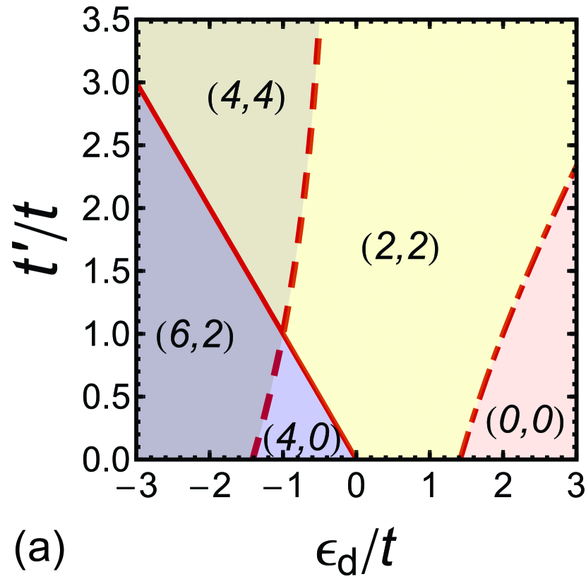
Figure 2: (Color online) Ground-state phase diagram of the isolated TTQD for $\Gamma\to 0$ and $U=0$ is plotted in (a) an $\epsilon_{d}$ vs $t^{\prime}$ plane for $\epsilon_{\mathrm{apex}}=\epsilon_{d}$, and in (b) an $\epsilon_{d}$ vs $\Delta\epsilon$ plane for $t^{\prime}=t$. Here, $\Delta\epsilon\equiv\epsilon_{\mathrm{apex}}-\epsilon_{d}$. The phase boundaries are given by the contours for the energy levels, crossing the Fermi level: $E_{\mathrm{o}}^{(1)}=0$ (solid line), $E_{\mathrm{e},+}^{(1)}=0$ (dashed line), and $E_{\mathrm{e},-}^{(1)}=0$ (dot-dashed line). The label ($N_{\mathrm{tot}}$, $\Theta$) is assigned for each region divided by these lines, and it represents the occupation number of the TTQD $N_{\mathrm{tot}}$, and $\Theta\equiv(\delta_{\mathrm{e}}-\delta_{\mathrm{o}})(2/\pi)$, which only for $U=0$ coincides with the difference in the occupation number of the even-parity levels and that of the odd-parity level.

The number of the electrons which enter the TTQD is determined by the relative position of these levels with respect to the Fermi energy $E_{F}$ ($=0$). Figure 2 shows the phase diagrams of the ground state of the TTQD cluster for $U=0$ and $\Gamma\to 0$. The boundaries are determined by the condition that the one-particle energy level crosses the Fermi energy: $E_{\mathrm{o}}^{(1)}=0$ (solid line), $E_{\mathrm{e},+}^{(1)}=0$ (dashed line), and $E_{\mathrm{e},-}^{(1)}=0$ (dot-dashed line). The left panel (a) is plotted as a function of $\epsilon_{d}$ and $t^{\prime}$ keeping the site diagonal part uniform $\epsilon_{\mathrm{apex}}=\epsilon_{d}$. Similarly, the right panel (b) is plotted as a function of $\epsilon_{d}$ and $\Delta\epsilon$ keeping the inter-dot couplings uniform $t^{\prime}=t$. Therefore, in the case of off-diagonal distortion, the cluster deforms from the regular triangle to a linear chain for $0\leq t^{\prime}<t$, and then for $t^{\prime}>t$ the coupling between the apex site and the other two becomes relatively weak as $t^{\prime}$ increases. The diagonal distortion $\epsilon_{\mathrm{apex}}\neq\epsilon_{d}$ affects directly the charge density in the apex site, and in Fig. 2 (b) the contour for the odd level becomes a vertical line because $E_{\mathrm{o}}^{(1)}$ does not depend on $\epsilon_{\mathrm{apex}}$.

The occupation number $N_{\mathrm{tot}}$, varies discontinuously as an energy level crosses the Fermi energy. For finite $\Gamma$, it can be deduced from the Friedel sum rule $(\delta_{\mathrm{e}}+\delta_{\mathrm{o}})(2/\pi)$. As shown in Fig. 2, it takes the values $N_{\mathrm{tot}}=0,\,2,\,4$, and $6$, depending on the region that is separated by the boundaries. The difference in the two phase shifts $\Theta\equiv(\delta_{\mathrm{e}}-\delta_{\mathrm{o}})(2/\pi)$ coincides, for $U=0$, with $N_{\mathrm{even}}-N_{\mathrm{odd}}$, where $N_{\mathrm{even}}$ and $N_{\mathrm{odd}}$ are the occupation number for the even and odd levels, respectively. In the limit of $\Gamma\to 0$, it can take the values of $\Theta=0,\,2$ and $4$ in the case of the TTQD, as shown in Fig. 2. For interacting electrons $U\neq 0$, however, there is no such general correspondence between $\Theta$ and the charge difference in the even and odd subspaces, while the Friedel sum rule remains valid. This is because the Coulomb interaction $\mathcal{H}_{\mathrm{dot}}^{U}$ breaks the charge conservation in each subspace, as seen explicitly in Eq. (33).

We also see in Fig. 2 that the odd-parity level $E_{\mathrm{o}}^{(1)}$ (solid line) and the excited even-parity level $E_{\mathrm{e},+}^{(1)}$ (dashed line) cross each other at $t=t^{\prime}$ and $\epsilon_{\mathrm{apex}}=\epsilon_{d}$, where the system has the full symmetry of the equilateral triangle. The crossing divides the region of four-electron occupation into two different spin-singlet regions, which can be classified according to the values of $\Theta$. In the region with $\Theta=0$ the highest occupied orbital is the odd-parity $b_{1}$ orbital, while in the opposite side with $\Theta=4$ the the even-parity orbital with energy $E_{\mathrm{e},+}^{(1)}$ becomes the highest occupied orbital. Note that the lowest even-parity orbital with energy $E_{\mathrm{e},-}^{(1)}$ has already been occupied by two electrons in this area of the parameter space.

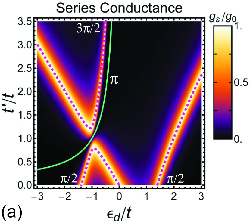
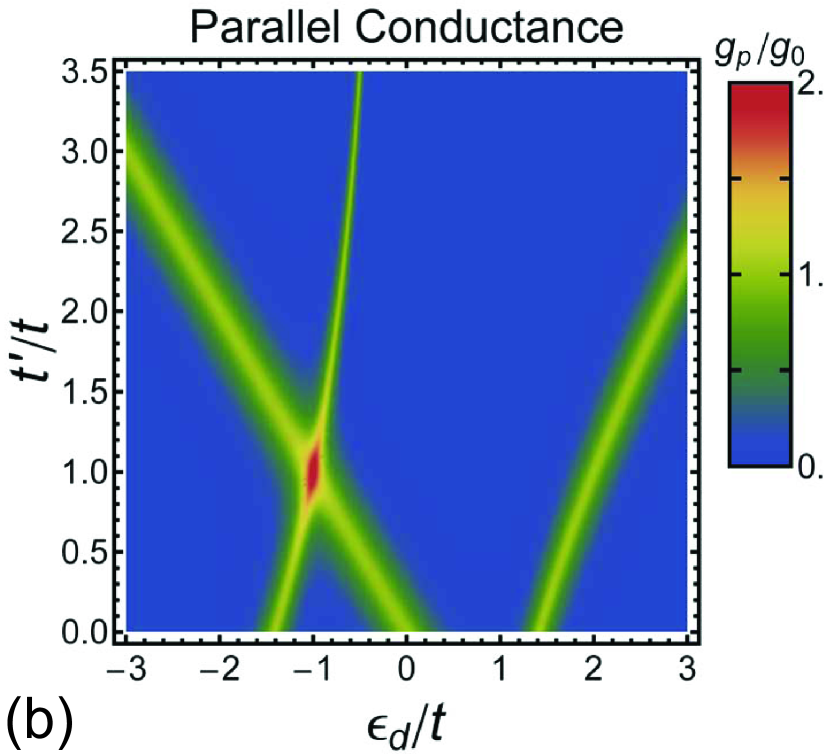
Figure 3: (Color online) Series (a) and parallel (b) conductances in the noninteracting case $U=0.0$ as functions of $\epsilon_{d}/t$ and $t^{\prime}/t$, for $\Gamma/t=0.25$ and $\epsilon_{\mathrm{apex}}=\epsilon_{d}$. The values of the conductances are scaled by $g_{0}\equiv 2e^{2}/h$. In (a) the solid line denotes the contour for $\delta_{\mathrm{e}}-\delta_{\mathrm{o}}=\pi$, and the dashed lines are the contours for the values of $\pi/2$ and $3\pi/2$.

III.2 Conductance for $U=0$

We next consider the noninteracting TTQD which are connected to the leads in a series or parallel configurations, as shown in Fig. 1. In this case, the conduction electrons from the leads are scattered at the TTQD. The phase shifts $\delta_{\mathrm{e}}$ and $\delta_{\mathrm{o}}$, caused by the scattering, are given by Eq. (11), replacing the renormalized parameters there by the bare ones $t$, $t^{\prime}$, and $\epsilon_{\mathrm{apex}}$. The conductance can be deduced from these phase shifts through Eqs. (6) and (8), or equivalently from the Green’s function using Eqs. (20) and (21) given in Appendix A.

The series and parallel conductances in the non-interacting case $U=0$ are plotted in Fig.  3 as functions of $\epsilon_{d}/t$ and $t^{\prime}/t$ for $\Gamma/t=0.25$ keeping the onsite potential for the three dots to be the same $\Delta\epsilon=0$. Similarly, in Fig. 4 the conductances are plotted as functions of $\epsilon_{d}/t$ and $\Delta\epsilon/t$, taking the inter-dot hopping matrix elements to be uniform $t^{\prime}=t$. The figures 3 and 4 can be compared, respectively, to the phase diagrams given in Fig. 2 (a) and (b).

Both $g_{\mathrm{s}}$ and $g_{\mathrm{p}}$ are enhanced as the resonance levels which correspond to the one-particle energies defined in Eq. (14) and (15) cross the Fermi level. The series and parallel conductances show a similar behavior in most of the parameter regions. We can see, however, that they show a quite different behavior at the point $t=t^{\prime}$ and $\Delta\epsilon=0$, where the series conductance vanishes while the parallel conductance takes the maximum possible value $g_{\mathrm{p}}=4e^{2}/h$ for two conducting channels. At this point, the two one-particle levels $E_{\mathrm{e},+}^{(1)}$ and $E_{\mathrm{o}}^{(1)}$ cross the Fermi level simultaneously, and the phase shifts take the value $\delta_{\mathrm{e}}=3\pi/2$ and $\delta_{\mathrm{o}}=\pi/2$.

The solid line in Fig. 3 (a) and Fig. 4 (a), denotes the contour of the difference in the two phase shifts for the value $\delta_{\mathrm{e}}-\delta_{\mathrm{o}}=\pi$. Thus, this contour corresponds to a zero line of the series conductance, and it means that destructive interference is most pronounced along this line. Similarly, the dashed lines in Fig. 3 (a) and Fig. 4 (a) are the contours for $\delta_{\mathrm{e}}-\delta_{\mathrm{o}}=\pi/2$ and $\,3\pi/2$, on which the two conductances show peaks of the same height $g_{\mathrm{s}}=2e^{2}/h$ and $g_{\mathrm{p}}=2e^{2}/h$.

We can also see in Figs. 3 and 4 that some conductance peaks are sharp and the others are relatively wide. Particularly, the resonance peak for the excited even-parity level $E_{\mathrm{e},+}^{(1)}$, which corresponds to the dashed line in Fig. 2 (a) and (b), is much sharper than the other peaks. This is because the eigenstate for $E_{\mathrm{e},+}^{(1)}$ has a large spectral weight at the apex site which has no direct couplings to the leads, and thus the hybridization with conduction band is suppressed. This feature can also be seen in the explicit expression for the spectral weight for the noninteracting TTQD is given in Eq. (31) in Appendix B. Conversely, the resonance width becomes large for the local states, the spectral weight of which is mainly on the other two dots coupled directly to the leads.

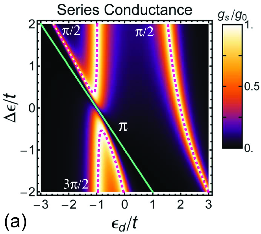
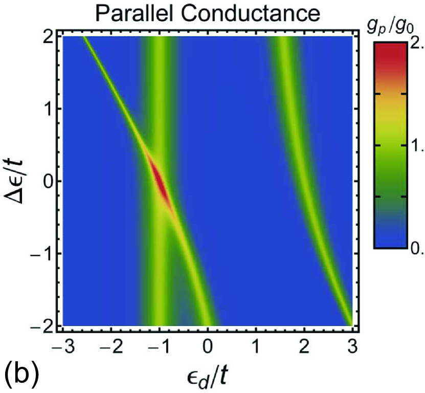
Figure 4: (Color online) Series (a) and parallel (b) conductances in the noninteracting case $U=0.0$ as functions of $\epsilon_{d}/t$ and $\Delta\epsilon/t$, for $\Gamma/t=0.25$ and $t^{\prime}=t$. Here, $\Delta\epsilon\equiv\epsilon_{\mathrm{apex}}-\epsilon_{d}$. The values of the conductances are scaled by $g_{0}\equiv 2e^{2}/h$. In (a) the solid line denotes the contour for $\delta_{\mathrm{e}}-\delta_{\mathrm{o}}=\pi$, and the dashed lines are the contours for the values of $\pi/2$ and $3\pi/2$.

IV Ground state in the molecular limit: $\Gamma=0$ and $U\neq 0$

The model can be solved also for finite Coulomb interaction $U$ in the molecular limit $\Gamma\to 0$.Numata2 ; KorkusinskiGimenezHawrylakETAL In this case the TTQD is disconnected from the leads, and described by the Hamiltonian,

$$\mathcal{H}_{\mathrm{dot}}\equiv\mathcal{H}_{\mathrm{dot}}^{0}+\mathcal{H}_{\mathrm{dot}}^{U}\;.$$ (16)

The eigenstates of $\mathcal{H}_{\mathrm{dot}}$ determine the high-energy properties of the system, particularly the properties of the local excitations near the quantum dots. It gives us a knowledge how the parameter space could be classified; such a classification relates to the fixed points of the renormalization group. In this section we examine the effects of the distortions on the local electronic states in the interacting case.

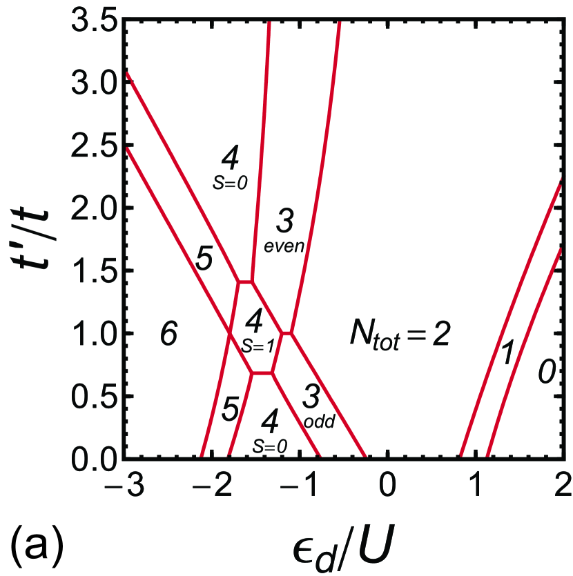
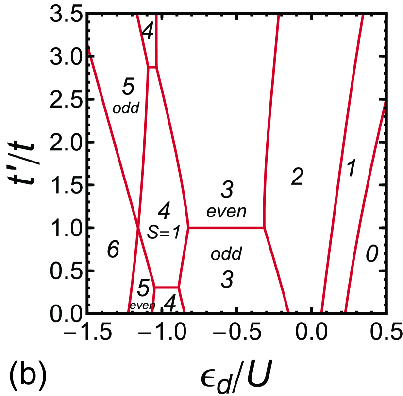
Figure 5: (Color online) Ground-state phase diagram of the TTQD for $\Gamma=0$ is plotted in a $\epsilon_{d}/U$ vs $t^{\prime}/t$ plane for $\Delta\epsilon=0$. The Coulomb interaction is chosen to be (a) $U/(2\pi t)=0.2$, and (b) $U/(2\pi t)=1.0$. The occupation number $N_{\mathrm{tot}}$ is shown for each region. The total spin $S$ is $1/2$ for odd $N_{\mathrm{tot}}$, and $S=0$ for even $N_{\mathrm{tot}}$, except it becomes $S=1$ in the middle of three $N_{\mathrm{tot}}=4$ regions. Along the horizontal line in the $N_{\mathrm{tot}}=3$ region, the ground state has an SU(4) symmetry due to the parity and spin degeneracies. The eigenstate has an even (odd) parity above (below) this horizontal line.

Figures 5 and 6 show the phase diagram of the ground state of the isolated TTQD for $\Gamma\to 0$. The Coulomb interaction is chosen to be (a) $U/(2\pi t)=0.2$, and (b) $U/(2\pi t)=1.0$. These figures can be compared with the phase diagrams in the non-interacting case shown in Fig. 2. We can see that the eigenstate with an odd-number of electrons ($N_{\mathrm{tot}}=1,\,3,$ and $5$) and total spin $S=1/2$ becomes a ground state due to the Coulomb interaction. The odd-number electron regions emerge between the even-number electron regions in the parameter space, and become wider as $U$ increases. We can also see that three horizontal border lines appear in the phase diagrams for $U>0$, and along each line a level crossing takes place between the two different eigenstates with the same occupation number.

The ground state for $N_{\mathrm{tot}}=3$ is separated by one of these horizontal lines at $t^{\prime}=t$ in Fig. 5, and similarly by the one at $\Delta\epsilon=0$ in Fig. 6. The ground state has an SU(4) symmetry along this border due to the orbital degeneracy caused by the symmetry of the equilateral triangle and the spin degeneracy. Away from this horizontal line, the distortions lower the equilateral symmetry, and lift the orbital degeneracy. An even-parity (odd-parity) state becomes the ground state for $t^{\prime}>t$ ($t^{\prime}<t$) in Fig. 5. Correspondingly, in Fig. 6 the ground state is an even-parity (odd-parity) state for $\epsilon_{\mathrm{apex}}<\epsilon_{d}$ ($\epsilon_{\mathrm{apex}}>\epsilon_{d}$). Note that there are some similarities between the phase diagrams in Fig. 5 and Fig. 6: the features seen for $t^{\prime}>t$ ($t^{\prime}<t$) are similar qualitatively (graphically) to those for $\Delta\epsilon<0$ ($\Delta\epsilon>0$). This is because the two types of the distortion, $t^{\prime}/t$ and $\epsilon_{\mathrm{apex}}-\epsilon_{d}$, lift the degeneracy in an opposite way, as mentioned in the above with Eqs. (14) and (15).

The Coulomb interaction also causes the high spin $S=1$ ground state seen in Figs. 5 and 6 in the middle of the $N_{\mathrm{tot}}=4$ regions where the TTQD has one extra electron introduced into the half-filled cluster. The $S=1$ region evolves in the parameter space from the level crossing point for $U=0$, seen in Fig. 2 at the point of $t^{\prime}=t$ and $\epsilon_{\mathrm{apex}}=\epsilon_{d}$. The degeneracy at this level crossing point is lifted for infinitesimal $U$, and the high-spin state evolves continuously, as $U$ increases, to the Nagaoka ferromagnetic state which is usually defined in the large $U$ limit. For large distortions, however, the transition to a singlet ground state takes place on the horizontal lines, running on the top and bottom of the $S=1$ region in Figs. 5 and 6.

The isolated TTQD which is not connected to the leads has a local moment of $S=1/2$ for odd-number fillings, and a high-spin $S=1$ for $N_{\mathrm{tot}}=4$, as mentioned in the above. In the case where two leads are coupled to the cluster, however, the local moment is screened eventually at low energies by the conduction electrons tunneling from the leads, and the ground state of the whole system becomes a spin singlet. We show the results of the ground-state properties of the TTQD connected to the leads in the next section, and then discuss also the characteristic energy scale of the Kondo screening in Sec. VI.

V NRG results for ground-state properties of the interacting TTQD

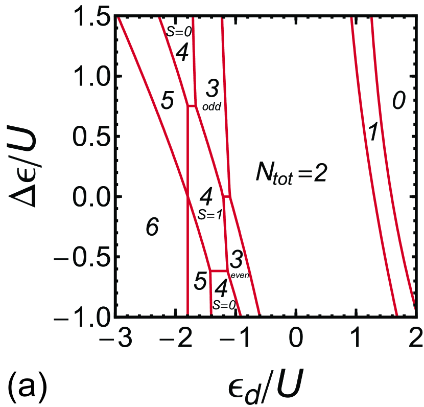
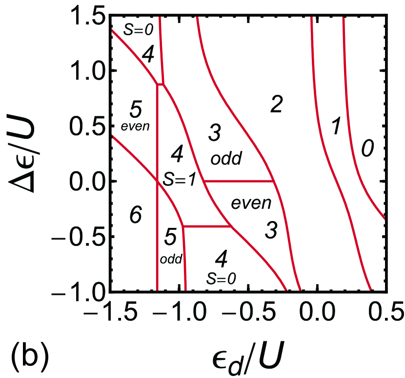
Figure 6: (Color online) Ground-state phase diagram of the TTQD for $\Gamma=0$ is plotted in a $\epsilon_{d}/U$ vs $\Delta\epsilon/U$ plane for $t^{\prime}=t$. The Coulomb interaction is chosen to be (a) $U/(2\pi t)=0.2$, and (b) $U/(2\pi t)=1.0$. The occupation number $N_{\mathrm{tot}}$ is shown for each region. The total spin $S$ is $1/2$ for odd $N_{\mathrm{tot}}$, and $S=0$ for even $N_{\mathrm{tot}}$, except it becomes $S=1$ in the middle of three $N_{\mathrm{tot}}=4$ regions. Along the horizontal line in the $N_{\mathrm{tot}}=3$ region, the ground state has an SU(4) symmetry due to the parity and spin degeneracies. The eigenstate has an odd (even) parity above (below) this horizontal line.

We now consider an interacting TTQD coupled to two leads via tunneling matrix elements $\mathcal{H}_{\mathrm{mix}}$ defined in Eq.  (4). In this case the phase shifts $\delta_{\mathrm{e}}$ and $\delta_{\mathrm{o}}$ play an central role on the low-energy properties. The effects of the Coulomb interaction enter through these two phase shifts, which can be expressed in terms of the renormalized parameters for the quasi-particles of the local Fermi liquid, as described in Eq. (11).

We have calculated the many-body phase shifts using the NRG method,Numata2 ; hewsonEPJ and have deduced the conductance and the occupation number of the TTQD at zero temperature from the phase shifts,Numata2 using Eqs.  (6)–(8). In our calculations, the ratio of the inter-dot hopping matrix element $t$ and the half width of the conduction band $D$, defined in Appendix C, is chosen to be $t/D=0.1$. The iterative diagonalization has been carried out by using the even-odd basis, described in Appendix B.Numata2 For constructing the Hilbert space in each NRG step, instead of adding two orbitals from even and odd orbitals simultaneously, we add one orbital from the even part first and retain 3600 low-energy states after carrying out the diagonalization of the Hamiltonian. Then, we add the other orbital from the odd part, and again keep the lowest 3600 eigenstates after the diagonalization. The discretization parameter is chosen to be $\Lambda=6.0$, which has been confirmed to reproduce the noninteracting results with a sufficient accuracy.OH ; ONH ; NO In the following, we set the strength of the Coulomb interaction to be $U/(2\pi t)=1.0$, which is adequate for observing typical results caused by $U$, as seen in Figs. 5 and 6. We have carried out some calculations changing $U$ and $\Gamma$ for the equilateral triangle in the previous work.Numata2 Our results have clarified how the value of $U$ affects the width of the Kondo ridges and the Kondo energy scale. Furthermore, a large $\Gamma$ smears the electronic structure of the TTQD origin. Through these observations, we have confirmed that the characteristic feature of the Kondo behavior can be seen clearly for typical a parameter set of $U/(2\pi t)=1.0$ and $\Gamma/t=0.12,\,0.25$.

V.1 Off-diagonal distortions: $\,t^{\prime}\neq t$

We discuss in this subsection the transport properties in the presence of the off-diagonal distortion $t^{\prime}\neq t$ keeping the site-diagonal potential uniform $\Delta\epsilon=0$. The effects of the diagonal distortion $\epsilon_{\mathrm{apex}}\neq\epsilon_{d}$ are examined in the next subsection V.2.

V.1.1 Local charge: $\,N_{\mathrm{tot}}=\frac{\displaystyle\mathstrut 2}{\displaystyle\mathstrut\pi}(\delta_{\mathrm{e}}+\delta_{\mathrm{o}})\,$ for $\,t\neq t^{\prime}$

Figure 7 shows the NRG results of the occupation number $N_{\mathrm{tot}}$ for $\Gamma/t=0.25$, and $U/(2\pi t)=1.0$. In (a), the results are plotted as a function of $\epsilon_{d}/U$ for several of values of $t^{\prime}/t$ ($=0.0,\,0.5,\,\ldots,$ and $3.5$, in steps of $0.5$). We can see clearly that the plateaus emerge near integer values of $N_{\mathrm{tot}}$ due to the Coulomb interaction, especially the one for $N_{\mathrm{tot}}\simeq 3.0$ becomes almost flat for large $t^{\prime}/t\gtrsim 3.0$. These results show that the coupling strength $\Gamma=0.25t$ is small enough to distinguish the different charge states for $U=2\pi t$. The plateau for the five-electron filling emerges due to the distortion and it becomes wider as $t^{\prime}/t$ deviates from $1.0$. These features are consistent with that for the isolated TTQD discussed in the above.

We have carried out the calculations more densely for a number of points in the parameter space than those presented in Fig.  7 (a), and the results are plotted in the $\epsilon_{d}/U$ vs $t^{\prime}/t$ plane in Fig.  7 (b). The dotted lines are the contours for $N_{\mathrm{tot}}=0.5,\,1.0,\,1.5,\,\ldots,$ and $5.5$ (in steps of $0.5$ from the right to the left). Note that this figure can be compared with Fig. 5 (b) where $N_{\mathrm{tot}}$ for $\Gamma\to 0$ is shown. We can see in Fig.  7 (b) that the contours of $N_{\mathrm{tot}}$ for half integers ($0.5$, $1.5$, …, and $5.5$), which are shown with the thicker dotted lines, follow almost faithfully the phase boundaries between the different charge states for $\Gamma\to 0$ shown in Fig. 5 (b). The electron filling $N_{\mathrm{tot}}$ changes rapidly near these contours for the half integers. This can be seen explicitly in Fig.  7 (a), and it reflects the fact that $\Gamma$ is much smaller than the inter dot matrix elements $t$ and the Coulomb interaction $U$ in the present case. From these observations, we see that the charge distribution in the plateaus regions is almost completely determined by the high energy states, and it can be approximated by the one in the limit of $\Gamma\to 0$. The low-lying energy states are required, however, to describe correctly the transport properties and the conduction-electron screening of the local moment of the TTQD.

 

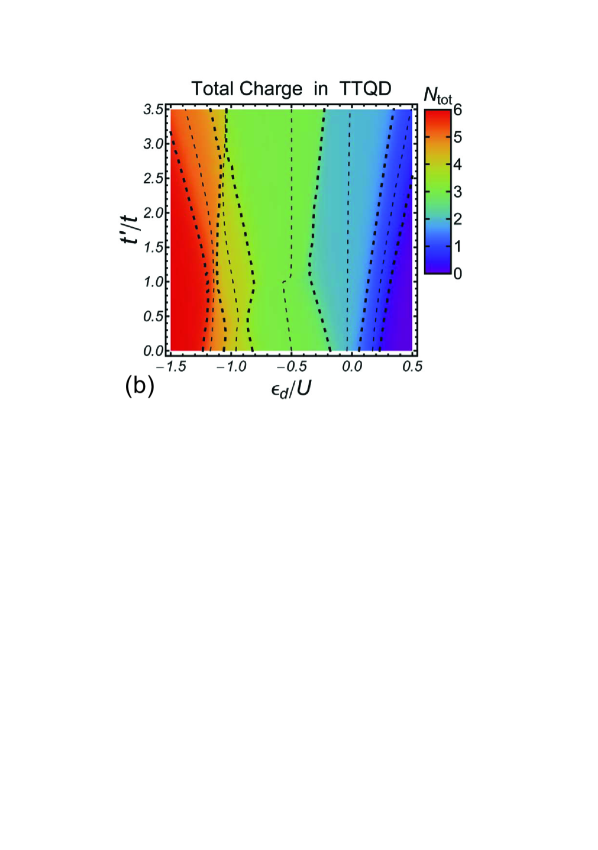
Figure 7: (Color online) NRG results for the occupation number $N_{\mathrm{tot}}$ for $U/(2\pi t)=1.0$, $\Gamma/t=0.25$, and $\Delta\epsilon=0$. The left panel (a) shows $N_{\mathrm{tot}}$ as a function of $\epsilon_{d}/U$ for $t^{\prime}/t=0.0,\,0.5,\,1.0,\ldots,$ and $3.5$. The right panel (b) shows $N_{\mathrm{tot}}$ in the $\epsilon_{d}/U$ vs $t^{\prime}/t$ plane. The dotted lines in (b) are the contours for $N_{\mathrm{tot}}=0.5,\,1.0,\,1.5,\,\ldots,$ and $5.5$ (in steps of $0.5$ from the right to the left).

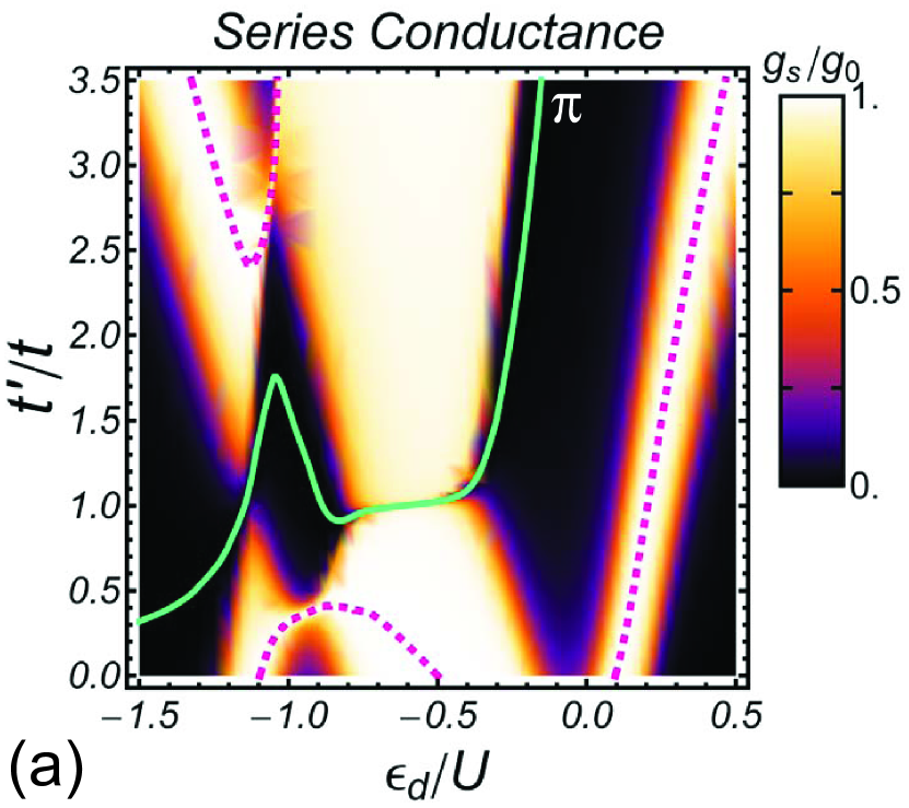
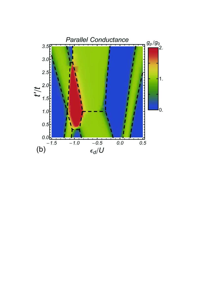
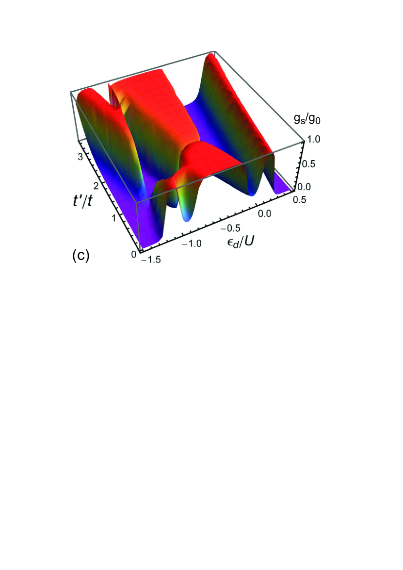
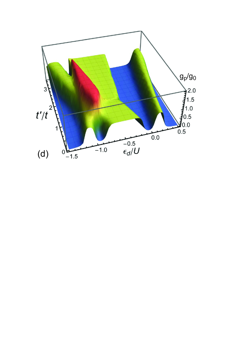
Figure 8: (Color online) Series (a) and parallel (b) conductances for $U/(2\pi t)=1.0$, $\Gamma/t=0.25$ and $\Delta\epsilon=0$ are plotted as functions of $\epsilon_{d}/U$ and $t^{\prime}/t$. In (a), the solid line is a contour for the phase-shift difference $\delta_{\mathrm{e}}-\delta_{\mathrm{o}}=\pi$, and the dotted lines are also the contours for $\delta_{\mathrm{e}}-\delta_{\mathrm{o}}=\pi/2$ and $3\pi/2$. In (b), the dashed lines denote the phase boundaries in the isolated limit $\Gamma\to 0$, corresponding to the ones shown in Fig. 5 (b). Lower panels: (c) and (d) are the surface plots of the series and parallel conductances corresponding to (a) and (b), respectively.

V.1.2 Series and Parallel Conductances for $\,t\neq t^{\prime}$

The NRG results for the conductances at zero temperature are shown in the $\epsilon_{d}/U$ vs $t^{\prime}/t$ plane in Fig.  8 for $U/(2\pi t)=1.0$, $\Gamma/t=0.25$, and $\Delta\epsilon=0$. In order to show more clearly the overall features, we have provided two types of the plots seen from different points in the parameter space for each of the conductances. The series conductance $g_{\mathrm{s}}$ is plotted in (a) and (c). Similarly, the parallel conductance $g_{\mathrm{p}}$ is shown in (b) and (d). For comparison, the phase boundary for $\Gamma\to 0$ given in Fig. 5 (b) is also superposed onto Fig.  8 (b) with the dashed lines. We see that the feature of the conductances reflects the occupation number in each of the regions in the parameter space. Note that the ground state becomes a spin singlet in the whole region of the parameter space due to the screening by the conduction electron.

We can also see in Figs.  8 (a) and (c) that typical Kondo ridges for the series conductance with $g_{\mathrm{s}}\simeq 2e^{2}/h$ emerge for odd-number fillings $N_{\mathrm{tot}}\simeq 1.0,\,3.0$, and $5.0$. Furthermore, both $g_{\mathrm{s}}$ and $g_{\mathrm{p}}$ almost vanish for even-number fillings $N_{\mathrm{tot}}\simeq 0.0,\,2.0$, $4.0$ and $6.0$ except for the $S=1$ Kondo region. Particularly, the behavior at small fillings $N_{\mathrm{tot}}\lesssim 2.0$, for $\epsilon_{d}/U\gtrsim-1.0$, can be explained simply by the $S=1/2$ Kondo effect due to the lowest single molecular orbital of $E_{\mathrm{e},-}^{(1)}$. Therefore, the characteristic features of the TTQD appear in the region of $\epsilon_{d}\lesssim-0.2U$, where the two excited levels $E_{\mathrm{o}}^{(1)}$ and $E_{\mathrm{e},+}^{(1)}$ are partially filled.

The solid line in Fig.  8 (a) denotes the contour for the difference in the two phase shifts corresponding to the value $\delta_{\mathrm{e}}-\delta_{\mathrm{o}}=\pi$. Along this line, the series conductance becomes exactly zero. Specifically, in the three-electron region, for $-0.8\lesssim\epsilon_{d}/U\lesssim-0.3$, this contour runs near the horizontal line for $t^{\prime}/t=1.0$ where the triangle has the equilateral symmetry. The contour line tilts slightly from the horizontal line because the coupling to the two leads breaks the equilateral symmetry already at $t^{\prime}=t$. This contour for $\delta_{\mathrm{e}}-\delta_{\mathrm{o}}=\pi$ appears in Fig.  8 (c) as a very sharp valley of the series conductance. The Kondo ridges on each side of this valley have a different parity. Just at the bottom of the valley, the low-lying quasi-particle states for the even and odd channels become degenerate, and the low-energy properties can be described by the SU(4) Fermi-liquid theory.Numata2 Furthermore, along this valley the two phase shifts are almost constant with the values, $\delta_{\mathrm{o}}\simeq\pi/4$ and $\delta_{\mathrm{e}}\simeq 5\pi/4$, since the Coulomb interaction keeps the sum of the two to be $\delta_{\mathrm{e}}+\delta_{\mathrm{o}}\simeq 3\pi/2$ in the three-electron region through the Friedel sum rule. Therefore, the parallel conductance does not change so much near this valley of the series conductance, keeping the value of $g_{\mathrm{p}}\simeq 2e^{2}/h$.

In order to see the sharp SU(4) Kondo valley in more detail, the conductances and the phase shifts at $\epsilon_{d}=-0.6U$ are plotted in Fig. 9 as functions of $t^{\prime}/t$. Particularly, the two lines in Fig. 9 (a) correspond to a cross section of the surface plots given in Fig.  8 (c) and (d) in the middle of the three-electron region along the vertical direction. We can see in Fig. 9 (b) that the phase-shift difference $\delta_{\mathrm{e}}-\delta_{\mathrm{o}}$ increases with $t^{\prime}/t$ showing a kink, the value of which varies from $\pi/2$ to $3\pi/2$ as $t^{\prime}/t$ increases, and taking the value of $\pi$ at $t^{\prime}/t\simeq 1.0$ in the middle of the transient region. This kink determines the structure of the series conductance valley seen in Fig. 9 (a). Therefore, the slope of the phase difference $\delta_{\mathrm{e}}-\delta_{\mathrm{o}}$ in the middle of the kink determines the width of the valley. Note that it is quite general to the local Fermi-liquid systems that the derivative of the phase shift with respect to the parameters, such as the frequency and the external fields, plays an important role on the renormalization of some correlation functions.

 

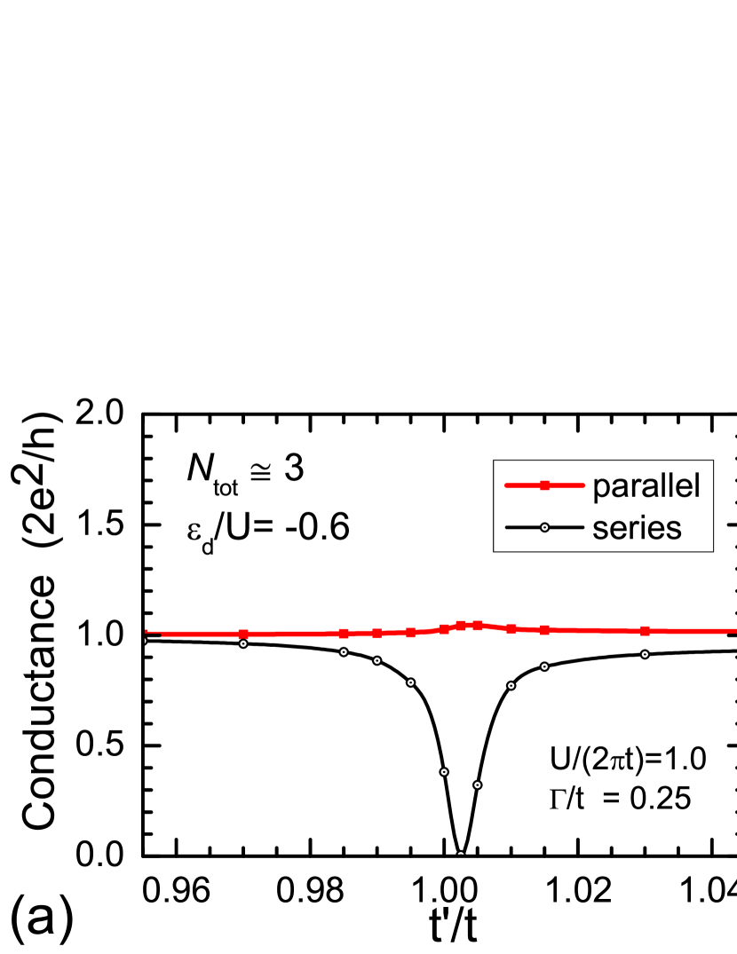
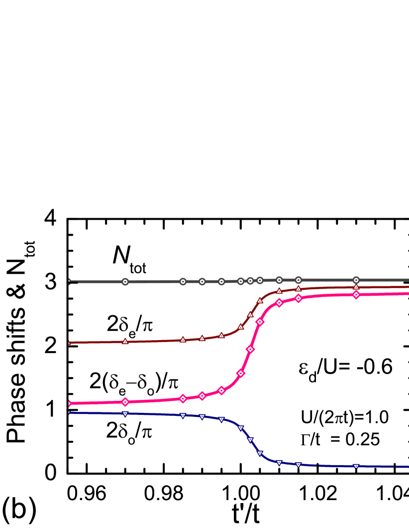
Figure 9: (Color online) Ground-state properties at $\epsilon_{d}=-0.6U$, (a) conductances and (b) phase shifts $(\delta_{\mathrm{e}}\pm\delta_{\mathrm{o}})(2/\pi)$, are plotted in a narrow region of $t^{\prime}$ near $t^{\prime}/t=1.0$ for $U/(2\pi t)=1.0$, $\Gamma/t=0.25$, and $\epsilon_{\mathrm{apex}}=\epsilon_{d}$. In this parameter region, the occupation number is almost constant $N_{\mathrm{tot}}\simeq 3.0$.

The $S=1$ Kondo behavior can be seen for the four-electron filling in the diamond-shape region in Figs.  8 (a) and (b). The series conductance almost vanishes $g_{\mathrm{s}}\simeq 0.0$ in this region, while the parallel conductance is enhanced $g_{\mathrm{p}}\simeq 4e^{2}/h$ despite an even-number electron filling. This contrast between $g_{\mathrm{s}}$ and $g_{\mathrm{p}}$ can be seen clearly, particularly in Figs.  8 (c) and (d). We can also see in Fig.  8 (a) that the contour for $\delta_{\mathrm{e}}-\delta_{\mathrm{o}}=\pi$ is winding in the center of the diamond region near $\epsilon_{d}/U\simeq-1.0$. Such a bend is not seen in the noninteracting case, for which the contour varies monotonically as shown in Fig. 3 (a). The contour lines of the phase shifts evolve, however, continuously from the non-interacting form. This is because the ground state of the whole system evolves adiabatically from a singlet described by a single Slater determinant to a correlated singlet described by the local Fermi-liquid theory for finite $\Gamma$. Note that the $S=1$ moment is screened at low temperature by the conduction electrons from the two leads via a two-stage screening processes.ONTN ; Numata ; Numata2

The dotted lines in Fig. 8 (a) express the contours for $\delta_{\mathrm{e}}-\delta_{\mathrm{o}}=\pi/2$ (below the solid line) and $3\pi/2$ (above the solid line), on which the series conductance reaches the unitary-limit value $g_{\mathrm{s}}=2e^{2}/h$. One of the dotted lines on the right, at $\epsilon_{d}/U\gtrsim 0.1$, follows simply the Kondo ridge caused by the lowest orbital $E_{\mathrm{e},-}^{(1)}$. The other two lines pass on the top and bottom of the diamond of the $S=1$ Kondo region. These two contours can be compared to the phase boundaries for the singlet-triplet transition, seen in a narrow range of $\epsilon_{d}$ at $t^{\prime}/t\simeq 0.30$ and $2.88$ in Fig. 5 (b). In order to clarify the precise feature of the corresponding crossover between the $S=1$ Kondo and non-Kondo singlet states, the conductance and phase shifts are plotted in Fig. 10 as functions of $t^{\prime}/t$, choosing the level position $\epsilon_{d}$ to be in the middle of the four-electron region at $\epsilon_{d}\simeq-1.04U$. At each of the crossover points, near $t^{\prime}/t\simeq 0.3$ and $3.0$, the series conductance has a peak. The feature of these conductance peaks reflects the kink in the phase difference $\delta_{\mathrm{e}}-\delta_{\mathrm{o}}$, the value of which varies from $0.2\pi$ to $1.0\pi$ near $t^{\prime}/t\simeq 0.3$, and from $1.0\pi$ to $3.0\pi$ near $t^{\prime}/t\simeq 3.0$. Therefore, the slope of these kink determines the width of the conductance of peak. Furthermore at the crossover region, the electron occupation fluctuates slightly from $4.0$ as $N_{\mathrm{tot}}-4.0\simeq\pm 0.5$. In the $S=1$ Kondo-singlet region situating between the two peaks of $g_{\mathrm{s}}$, the phase shifts are almost locked at $\delta_{\mathrm{e}}\simeq 3\pi/2$ and $\delta_{\mathrm{o}}\simeq\pi/2$, and thus the parallel conductance takes the value $g_{\mathrm{p}}=4e^{2}/h$. In one of the non-Kondo regions for $t^{\prime}/t\gtrsim 3.2$, the phase shifts approach to $\delta_{\mathrm{e}}\simeq 2\pi$ and $\delta_{\mathrm{o}}\simeq 0$. The phase shifts take the values of $\delta_{\mathrm{e}}\simeq 1.2\pi$, and $\delta_{\mathrm{o}}\simeq\pi$ in the limit of $t^{\prime}\to 0$, in the other non-Kondo region for $t^{\prime}/t\lesssim 0.2$. Note that for Fig. 10, the coupling between the TTQD and the leads has been chosen to be $\Gamma/t=0.12$, which is smaller than that ($\Gamma/t=0.25$) for the previous figures, in order to see clearly the typical features of the narrow crossover regions.

 

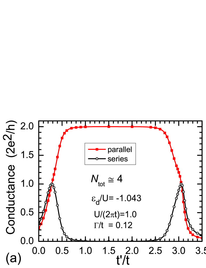
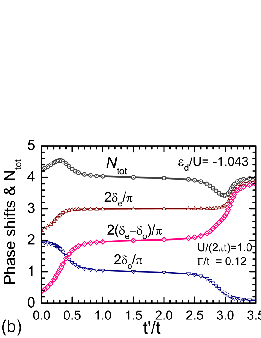
Figure 10: (Color online) Ground-state properties at $\epsilon_{d}=-1.043U$, (a) conductances and (b) phase shifts $(\delta_{\mathrm{e}}\pm\delta_{\mathrm{o}})(2/\pi)$, are plotted as functions of $t^{\prime}/t$ for $U/(2\pi t)=1.0$, $\Gamma/t=0.12$, and $\epsilon_{\mathrm{apex}}=\epsilon_{d}$. In this parameter region, the occupation number is almost constant $N_{\mathrm{tot}}\simeq 4.0$. Note that in the limit of $\Gamma\to 0$ the Nagaoka state is the ground state for the isolated cluster for $0.30<t^{\prime}/t<2.88$.

V.1.3 Phase-shift difference: $\,\Theta=\frac{\displaystyle\mathstrut 2}{\displaystyle\mathstrut\pi}(\delta_{\mathrm{e}}-\delta_{\mathrm{o}})\,$ for $\,t\neq t^{\prime}$

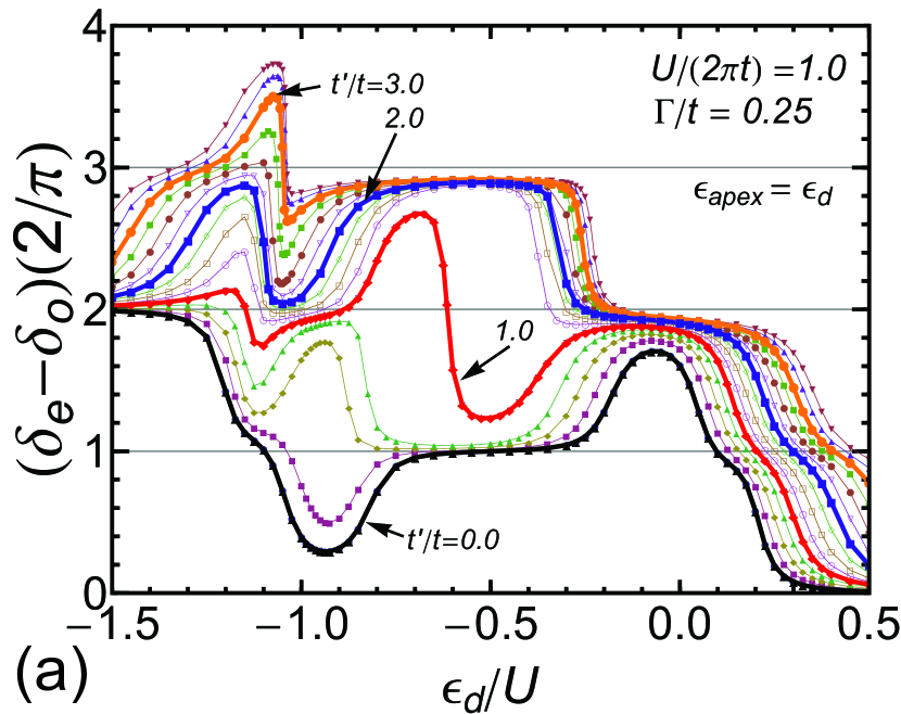
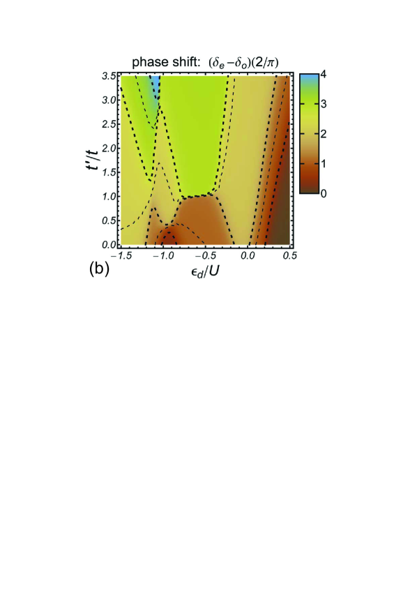
Figure 11: (Color online) Difference between the even and odd phase shifts $\Theta\equiv(\delta_{\mathrm{e}}-\delta_{\mathrm{o}})(2/\pi)$ for $U/(2\pi t)=1.0$, $\Gamma/t=0.25$ and $\Delta\epsilon=0$. The left panel (a) shows $\Theta$ as a function of $\epsilon_{d}/U$ for the values of $t^{\prime}/t=0.0,\,0.25,\,0.5,\ldots,$ and $3.5$ (in steps of $0.25$ from the bottom to the top). The right panel (b) shows $\Theta$ in the $\epsilon_{d}/U$ vs $t^{\prime}/t$ plane. The dotted lines in (b) are the contours for $(\delta_{\mathrm{e}}-\delta_{\mathrm{o}})(2/\pi)=0.5,\,1.0,\,1.5,\,\ldots,$ and $3.5$ (in steps of $0.5$ from the bottom to the top).

The difference between the two phase shifts $\delta_{\mathrm{e}}-\delta_{\mathrm{o}}$ is a fundamental parameter that contains the essential information of the interference effects between the even and odd conducting channels. It affects the series conductance, while each channel contributes independently to the parallel conductance, through the expressions given in eqs. (6) and (8). Specifically, peaks and dips of the series conductance correspond directly to the kinks of the phase-shift difference $\delta_{\mathrm{e}}-\delta_{\mathrm{o}}$, as seen in Figs. 9 and 10. It is also much easier for a numerical purpose to trace the kink structure of $\delta_{\mathrm{e}}-\delta_{\mathrm{o}}$ than to find directly the dips and peaks of $g_{\mathrm{s}}$.

We also provide the NRG results for $\Theta\equiv(\delta_{\mathrm{e}}-\delta_{\mathrm{o}})(2/\pi)$ in Fig. 11 in order to clarify its behavior in the wide parameter space. In the left panel (a), $\Theta$ is plotted as a function of $\epsilon_{d}/U$ for the values of $t^{\prime}/t$ varying from $0.0$ to $3.5$ in steps of $0.25$. Furthermore, Fig. 11 (b) shows the results obtained in the $\epsilon_{d}/U$ vs $t^{\prime}/t$ plane: the dotted lines are the contours for the values of $\Theta$ varying from $0.5$ (bottom and right) to $3.5$ (top) in steps of $0.5$. We can see that there are several plateaus, or shelves, in these figures near the integer values of $\Theta\simeq 1.0,\,2.0,$ and $3.0$, on which $g_{\mathrm{s}}$ becomes almost transparent or zero. Furthermore, the occupation number also approaches to an integer value on each of these plateaus, and thus they can be classified according to a set of the two integers $(N_{\mathrm{tot}},\,\Theta)$. For instance, in Fig. 11 (a), we can see a wide plateau which can labelled by $(N_{\mathrm{tot}},\,\Theta)\simeq(3.0,\,3.0)$ for $-1.0\lesssim\epsilon_{d}/U\lesssim-0.3$ and $t^{\prime}/t\gtrsim 1.0$. The height of the plateau, however, is still somewhat smaller than the exact integer $3.0$. Such a deviation of the plateau height from an integer value decreases as $\Gamma$ decreases. This has been confirmed explicitly for the equilateral triangle in the previous work [see Fig. 6 of Ref. Numata2, ]. Furthermore, we can see another example for smaller $\Gamma$ in the next section [see Fig. 14].

The feature of $\Theta$ in the parameter space can also be compared to the phase diagram for the isolated TTQD. Particularly, the contours for $\Theta=0.5,\,1.5,\,2.5,\,$ and $3.5$, which are shown with the thicker dotted lines in Fig. 11 (b), divide the parameter space in a similar way that the phase boundaries did in Fig. 5 (b). The contour lines, however, do not cross each other while the border lines for $\Gamma=0$ are crossing at some points. We can see in Fig. 11 that the SU(4) Kondo effect is manifest in the parameter space as a sheer cliff at $-0.8\lesssim\epsilon_{d}/U\lesssim-0.3$ near $t^{\prime}/t\simeq 1.0$. It also corresponds to the kink that we have seen in Fig. 9 (b). Between the bottom and top of the cliff the value of $\Theta$ varies from $1.0$ to $2.9$, respectively. The slope of the cliff determines the width of the SU(4) valley which corresponds to the contour line for $\Theta=2.0$, running in the middle of the cliff. The Kondo ridges of $g_{\mathrm{s}}$ on both sides of the valley can be classified according to the plateau value of $\delta_{\mathrm{e}}-\delta_{\mathrm{o}}=\pi/2$ or $3\pi/2$, as the phase difference varies by $\pi$ across the valley.

The $S=1$ Kondo region can also be seen as a diamond-shape plateau in Fig. 11 (b), appearing at $\epsilon_{d}\simeq-1.0U$ and $0.3\lesssim t^{\prime}/t\lesssim 2.9$. This plateau is characterized by the two parameters, $\Theta\simeq 2.0$ and $N_{\mathrm{tot}}\simeq 4.0$. Thus the phase shifts are almost fixed at the value of $\delta_{\mathrm{e}}\simeq 3\pi/2$ and $\delta_{\mathrm{o}}\simeq\pi/2$ in this region.

V.2 Diagonal distortions: $\epsilon_{\mathrm{apex}}\neq\epsilon_{d}$

We next examine the effects of the diagonal distortion $\epsilon_{\mathrm{apex}}\neq\epsilon_{d}$, keeping the inter-dot hopping matrix elements uniform $t^{\prime}=t$ and taking the Coulomb interaction to be $U=2\pi t$. In this subsection we choose the coupling between the leads and the TTQD such that $\Gamma/t=0.12$, which is approximately a half of the one used for Figs.  7, 8 and 11 in the off-diagonal case.

V.2.1 Local charge: $\,N_{\mathrm{tot}}=\frac{\displaystyle\mathstrut 2}{\displaystyle\mathstrut\pi}(\delta_{\mathrm{e}}+\delta_{\mathrm{o}})\,$ for $\,\Delta\epsilon\neq 0$

 

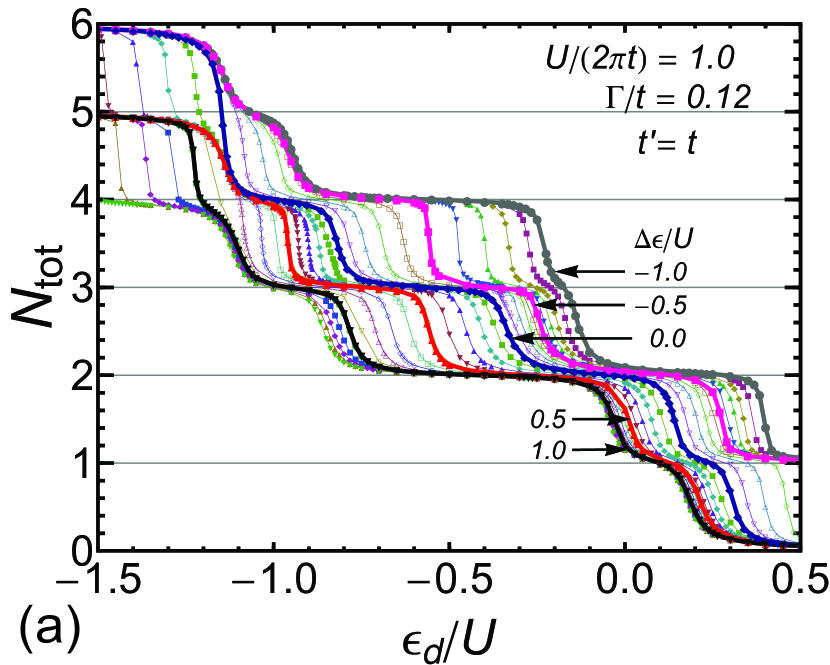
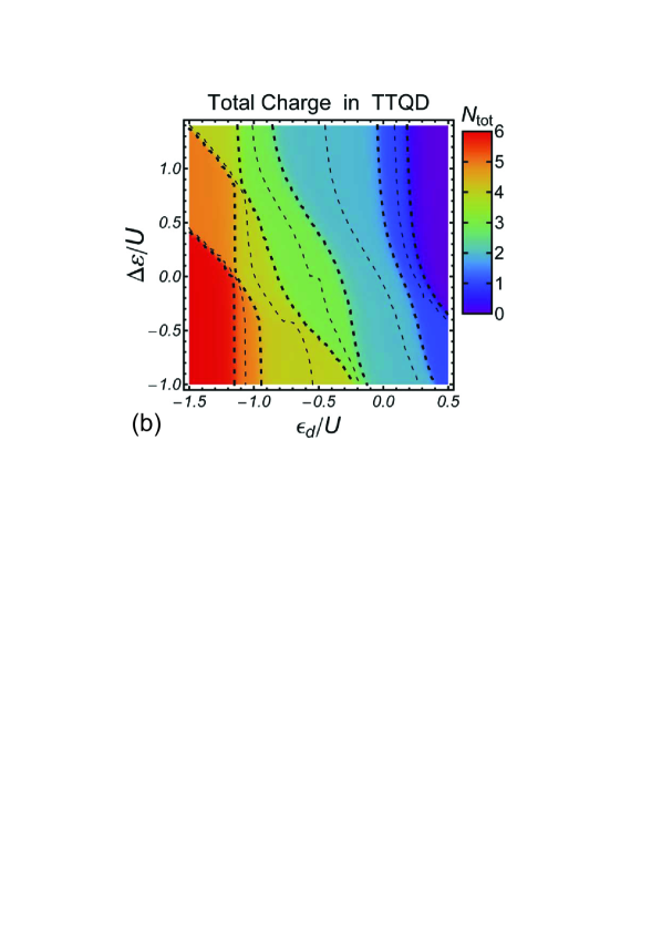
Figure 12: (Color online) NRG results of the occupation number $N_{\mathrm{tot}}$ for $U/(2\pi t)=1.0$, for $\Gamma/t=0.12$ and $t^{\prime}=t$. The left panel (a) shows $N_{\mathrm{tot}}$ as a function of $\epsilon_{d}/U$ for values of for the values of $\Delta\epsilon/U=-1.0,\,-0.9,\,-0.8,\,\ldots,$ and $1.4$ (in steps of $0.1$ from the top to the bottom). The right panel (b) shows $N_{\mathrm{tot}}$ in the $\epsilon_{d}/U$ vs $\Delta\epsilon/U$ plane. The dotted lines in (b) are the contours for $N_{\mathrm{tot}}=0.5,\,1.0,\,1.5,\,\ldots,$ and $5.5$ (in steps of $0.5$ from the right to the left).

Figure 12 (a) shows the occupation number $N_{\mathrm{tot}}$ in the TTQD as a function of $\epsilon_{d}/U$ for the values of $\Delta\epsilon/U=-1.0,\,-0.9,\,-0.8,\,\ldots,$ and $1.4$ (in steps of $0.1$ from the top to the bottom). We can see clearly that the plateaus appear near integer values of $N_{\mathrm{tot}}$. In the present case the coupling strength $\Gamma$ is much smaller than $U$ and $t$, so that the different charge states can be distinguished clearly. In other words, the crossover between two adjacent charge states becomes sharp, and thus the border can be determined reasonably by the middle point where $N_{\mathrm{tot}}$ takes a half-integer value.

We have also carried out the calculations for a number of parameter sets, more than the ones which are shown explicitly in Fig. 12 (a), and have plotted the results in Fig.  12 (b) in the $\epsilon_{d}/U$ vs $\Delta\epsilon/U$ plane. In this figure the dotted lines denote the contours for $N_{\mathrm{tot}}=0.5,\,1.0,\,1.5,\,\ldots,$ and $5.5$ (in steps of $0.5$ from the right to the left). Particularly, the thick dotted lines are the contours for the half-integer values; $0.5$, $1.5$, $2.5$, $3.5$, $4.5$, and $5.5$. We can see that these thick dotted lines almost follow the phase boundaries between the different charge states in the isolated TTQD, shown in Fig. 6 (b). The local charge $N_{\mathrm{tot}}$ changes rapidly near these thick contours, and has a plateau of an integer value between the thick dotted lines, as can be seen explicitly in Fig.  12 (a). Therefore the charge in the plateau regions is determined at high energy scale, and the sum of the phase shifts $(2/\pi)(\delta_{\mathrm{e}}+\delta_{\mathrm{o}})$ in the plateaus can be approximated reasonably by the value of $N_{\mathrm{tot}}$ in the $\Gamma\to 0$ limit. However, the transport properties at zero temperature are determined by each of the two phase shifts or the difference between them, which are determined essentially by the low-lying energy states of the whole system including the leads.

V.2.2 Series and Parallel Conductances for $\,\Delta\epsilon\neq 0$

The series (a) and parallel (b) conductances are plotted in Fig.  13 in the parameter space of $\epsilon_{d}/U$ and $\Delta\epsilon/U$. For comparison, the phase diagram for $\Gamma\to 0$ given in Fig. 6 (b) is superposed onto Fig.  13 (b) with the dashed lines. We can see that the behavior of the conductances in this parameter space also reflects the feature of the phase diagram for the isolated TTQD. In the regions of the odd-number electron filling the both conductances $g_{\mathrm{s}}$ and $g_{\mathrm{p}}$ have the Kondo plateaus with the height of $2e^{2}/h$. Furthermore, the $S=1$ Kondo effect takes place in a trapezoidal region near $\Delta\epsilon\simeq 0.0$ and $\epsilon_{d}/U\simeq-1.0$. In this region, the series and parallel conductances show a clear contrast, namely $g_{\mathrm{s}}\simeq 0$ while $g_{\mathrm{p}}\simeq 4e^{2}/h$. This feature is the same as what is observed in the case of the off-diagonal distortions.

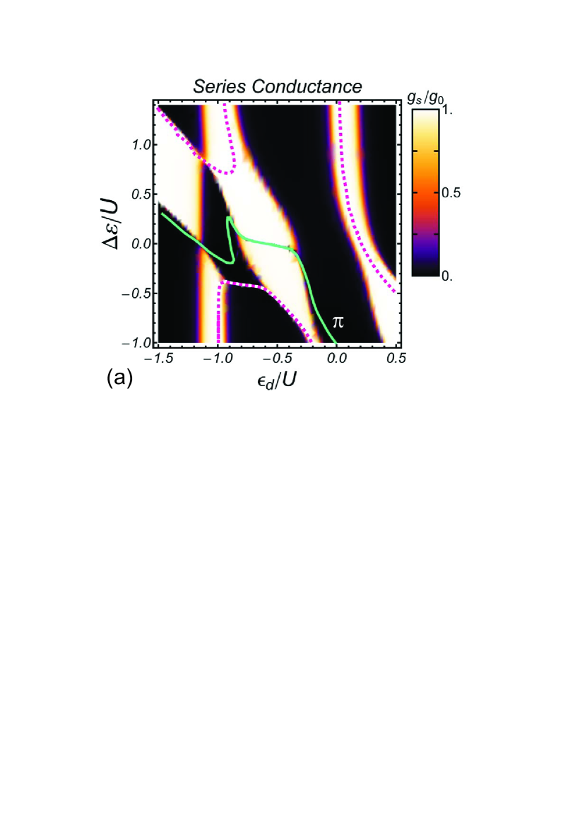
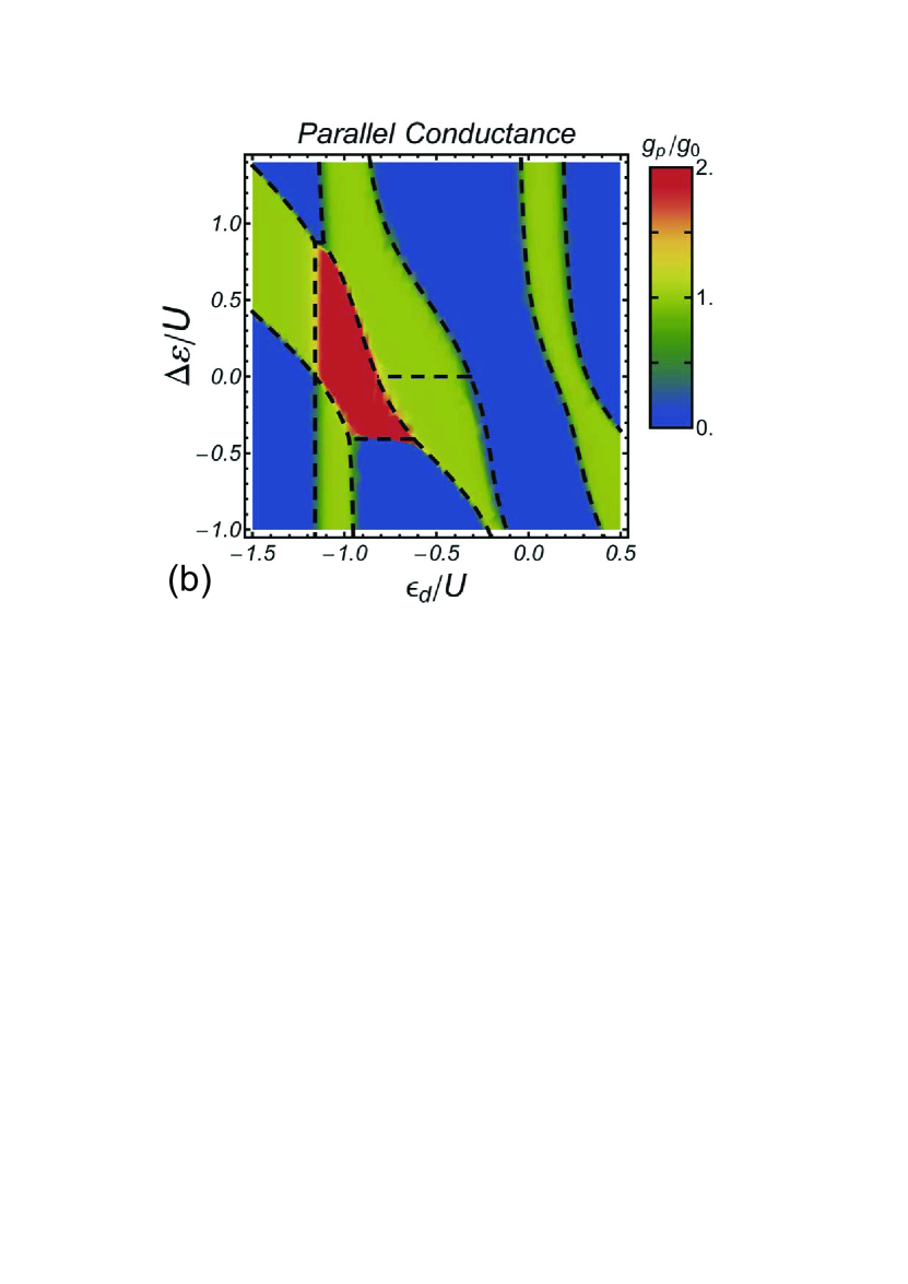
Figure 13: (Color online) Series (a) and parallel (b) conductances for $U/(2\pi t)=1.0$, $\Gamma/t=0.12$ and $t=t^{\prime}$ are plotted as functions of $\epsilon_{d}/U$ and $\Delta\epsilon/U$. In (a), the solid line is a contour for the phase-shift difference $\delta_{\mathrm{e}}-\delta_{\mathrm{o}}=\pi$, and the dotted lines are also the contours for the values of $\pi/2$ and $3\pi/2$. In (b), the dashed lines denote the phase boundaries for the isolated TTQD, corresponding to Fig. 6 (b).

The solid line in Fig.  13 (a) denotes the contour for $\delta_{\mathrm{e}}-\delta_{\mathrm{o}}=\pi$, on which the series conductance becomes zero. This contour runs across the region of the three-electron occupancy almost horizontally in an area with weak distortions $\Delta\epsilon\simeq 0.0$. It associated with a sharp valley of the series conductance, which is typical of the SU(4) Kondo effect in the TTQD and is seen also for the off-diagonal distortions. The SU(4) symmetry is caused by the channel degeneracy restored along the line at low energies,Numata2 and the phase shifts take the values of $\delta_{\mathrm{e}}\simeq 5\pi/4$ and $\delta_{\mathrm{o}}\simeq\pi/4$. We can also see that the contour for $\delta_{\mathrm{e}}-\delta_{\mathrm{o}}=\pi$ is deformed significantly, in the trapezoidal $S=1$ Kondo region, from the non-interacting form which is a simple straight line shown in Fig. 4 (a). This could happen, however, continuously with increasing $U$, as the ground state evolves adiabatically in the case that the quantum dots are coupled to the leads.

The dotted lines in Fig.  13 (a) denote the contours for $\delta_{\mathrm{e}}-\delta_{\mathrm{o}}=\pi/2$ (above the solid line) and $3\pi/2$ (below the solid line), on which the series conductance takes the unitary-limit value $g_{\mathrm{s}}=2e^{2}/h$. It should be noted that a long and very sharp ridge emerges in Fig.  13 (a) for the series conductance at $\Delta\epsilon/U\simeq-0.4$ and $-0.9\lesssim\epsilon_{d}/U\lesssim-0.6$. This sharp ridge runs along the lower end of the trapezoidal $S=1$ Kondo region, and reflects the singlet-triplet transition taking place in the isolated TTQD cluster for $\Gamma\to 0$.

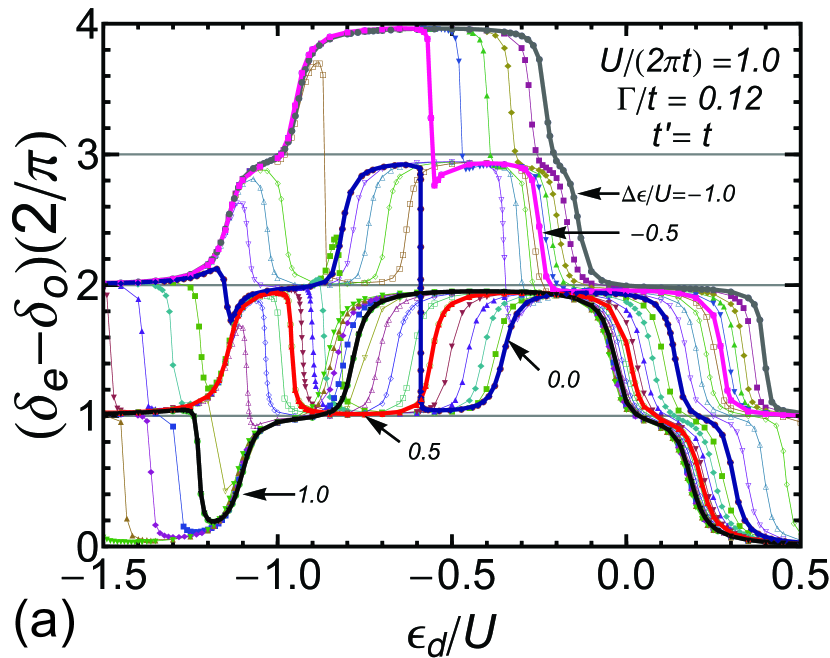
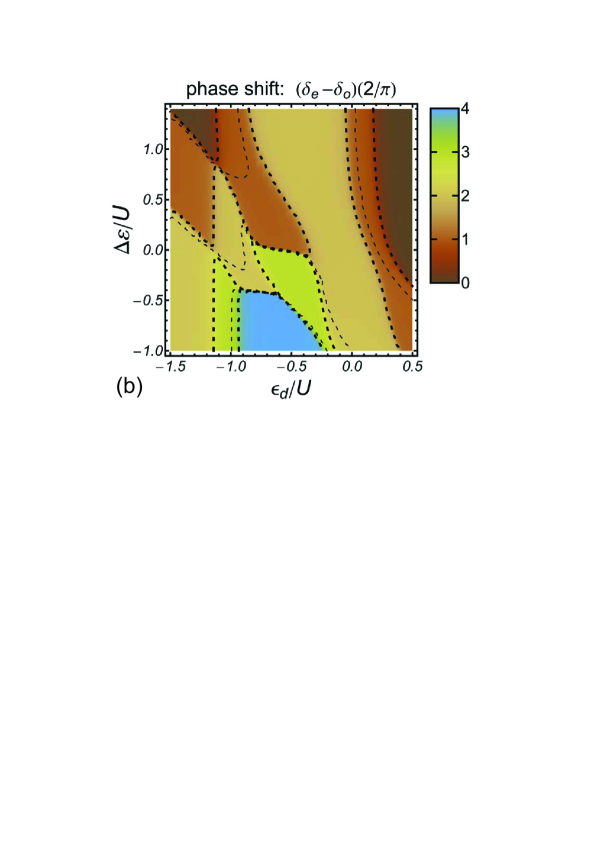
Figure 14: (Color online) Difference between the even and odd phase shifts $\Theta\equiv(\delta_{\mathrm{e}}-\delta_{\mathrm{o}})(2/\pi)$ for $U/(2\pi t)=1.0$, $\Gamma/t=0.12$ and $t^{\prime}=t$. The left panel (a) shows $\Theta$ as a function of $\epsilon_{d}/U$ for the values of $\Delta\epsilon/U=-1.0,\,-0.9,\,-0.8,\,\ldots,$ and $1.4$ (in steps of $0.1$ from the top to the bottom). The right panel (b) shows $\Theta$ in the $\epsilon_{d}/U$ vs $\Delta\epsilon/U$ plane. The dotted lines in (b) are the contours for $(\delta_{\mathrm{e}}-\delta_{\mathrm{o}})(2/\pi)=0.5,\,1.0,\,1.5,\,\ldots,$ and $3.5$ (in steps of $0.5$ from the top to the bottom).

V.2.3 Phase-shift difference: $\,\Theta=\frac{\displaystyle\mathstrut 2}{\displaystyle\mathstrut\pi}(\delta_{\mathrm{e}}-\delta_{\mathrm{o}})\,$ for $\,\Delta\epsilon\neq 0$

Figure 14 (a) shows the results of the phase-shift difference $\Theta\equiv(\delta_{\mathrm{e}}-\delta_{\mathrm{o}})(2/\pi)$ as a function of $\epsilon_{d}/U$ for the values of $\Delta\epsilon/U$ varying from $-1.0$ to $1.4$ in steps of $0.1$. We can clearly see that there are a number of plateaus near integer values of $\Theta\simeq 1.0,\,2.0,$ and $3.0$. Specifically, the height of the plateaus approaches very close to exact integers in the present case because the coupling between the leads and the TTQD is small. Although we can recognize that some of them, for instance, the ones near $\Theta\simeq 3.0$, still deviate from an exact integer, these deviations can be controlled by tuning $\Gamma$ to be small. Numata2

In order to see the behavior of $(\delta_{\mathrm{e}}-\delta_{\mathrm{o}})(2/\pi)$ in the parameter space, the results are plotted also in the $\epsilon_{d}/U$ vs $\Delta\epsilon/U$ plane in Fig. 14 (b). In this figure the dotted lines denote the contours for $\Theta$, particularly the thicker ones are the contours for the half-integer values: $\Theta=0.5$, $1.5$, $2.5$, and $3.5$. Each of these thick dotted lines runs very closed to the phase boundaries for the isolated TTQD shown in Fig. 6 (b). These thick contours, as a whole, cover almost all the boundaries. These contour lines of $\Theta$, however, evolve continuously from the non-interacting forms as $U$ increases. This is because the ground state of the whole system evolve adiabatically from a $U=0$ spin singlet to a correlated singlet described the local Fermi-liquid theory for finite $\Gamma$.

The sharp SU(4) Kondo valley of the series conductance corresponds to a steep cliff standing at $-0.8\lesssim\epsilon_{d}/U\lesssim-0.3$ for small distortions $\Delta\epsilon/U\simeq 0.0$ in Fig. 14 (b). At the edge of this cliff, $(\delta_{\mathrm{e}}-\delta_{\mathrm{o}})(2/\pi)$ varies by an amount $2.0$ approximately. It varies from $\Theta\simeq 1.0$ (for $\Delta\epsilon\gtrsim 0.0$) to $\Theta\simeq 2.9$ (for $\Delta\epsilon\lesssim 0.0$), taking the value of $\delta_{\mathrm{e}}-\delta_{\mathrm{o}}=\pi$ which corresponds to the zero point of $g_{\mathrm{s}}$ in the middle of the cliff. The slope of this cliff determines the width of the SU(4) valley, as that in the case of off-diagonal distortions.

We can see another sharp cliff in Fig. 14 (b) at the bottom of the $S=1$ Kondo region for $\Delta\epsilon/U\simeq-0.4$ and $-0.9\lesssim\epsilon_{d}/U\lesssim-0.6$, where the singlet-triplet transition takes place for the isolated cluster. Between the top and bottom of this cliff, the phase difference $\Theta$ varies rapidly from $2.0$ to $4.0$, which causes the sharp Kondo ridge of the series conductance, seen in Fig.  13 (a). Note that the slope of the cliff determines the width of the sharp peak of $g_{\mathrm{s}}$. We can also see a narrow cliff due to the singlet-triplet transition, at the top of the $S=1$ Kondo region for $\Delta\epsilon/U\simeq 0.8$ and $\epsilon_{d}/U\simeq-1.2$. At this cliff, the value of $\Theta$ changes from $0.0$ to $2.0$ approximately.

VI Characteristic energy scale

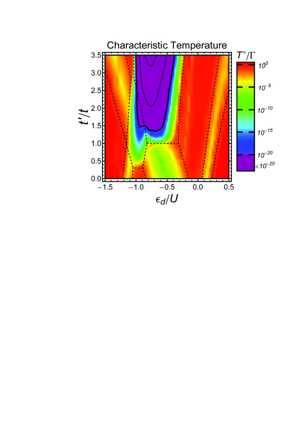
Figure 15: (Color online) The characteristic energy scale $T^{*}$ in the $\epsilon_{d}/U$ vs $t^{\prime}/t$ plane for $\Gamma/t=0.25$, $U/(2\pi t)=1.0$ and $\Delta\epsilon=0$. The results in the range of $-20<\log_{10}(T^{*}/\Gamma)<0$ are painted in the colors varying from blue to red. $T^{*}$ becomes very small in the purple region, and the solid lines there denote the contours for $\log_{10}(T^{*}/\Gamma)=-20,\,-40$, and $-60$. The dashed lines denote the phase boundary in the limit of $\Gamma\to 0$, corresponding to Fig. 5 (b).

The ground-state properties, discussed in the above, are determined by the behavior of the phase shifts for the quasi-particles. At finite temperature $T$, for instance, the structure of the plateaus and dips will be smeared gradually as $T$ increases. Nevertheless, the corrections due to finite $T$ can be still determined by the local Fermi-liquid theory for $T\lesssim T^{*}$, namely at temperatures lower than the characteristic energy scale $T^{*}$. Specifically, in the case the quantum dots have a local moment, $T^{*}$ can be regarded as the Kondo temperature such that the moment is screened at $T\ll T^{*}$. The value of $T^{*}$, however, depends sensitively on the parameters at each point of the parameter space. Therefore, the actual temperature, at which the Fermi-liquid behavior can be observed, is different depending on the region in the parameter space.

In the NRG approach, the crossover from the high energy to the low energy Fermi-liquid regime can be seen in the trajectory of the low-energy levels of the discretized Hamiltonian $H_{N}$ defined in Appendix C. The trajectory evolves as the number of orbitals $N$ of the conduction band increases. In the present work we have estimated $T^{*}$ through $N^{*}$ that is a particular value of $N$, at which the trajectory almost enters the low-energy regime, as

$$T^{*}=D\,\Lambda^{-(N^{*}-1)/2}\;.$$ (17)

Therefore, $T^{*}$ is the typical energy scale of the low-lying excitations of a finite NRG chain with $N=N^{*}$. The values of $T^{*}$ determined in this way have some ambiguities, especially in the case where the crossover is gradual, and our definition tends to give a smaller value for the characteristic energy scale. Nevertheless, the relative variations of $T^{*}$ in the parameter space can be extracted reasonably as shown in Figs. 15 and 18. We have also confirmed that $T^{*}$ determined in this way is consistent with the ones we had estimated from the entropy in the previous work for the equilateral triangle.Numata2 We will see below that the variations of $T^{*}$ can be understood roughly through the distribution of the charge and spin in the even and odd parity orbitals, described in Appendix B.

VI.1 $T^{*}$ vs off-diagonal distortions ($t^{\prime}\neq t$)

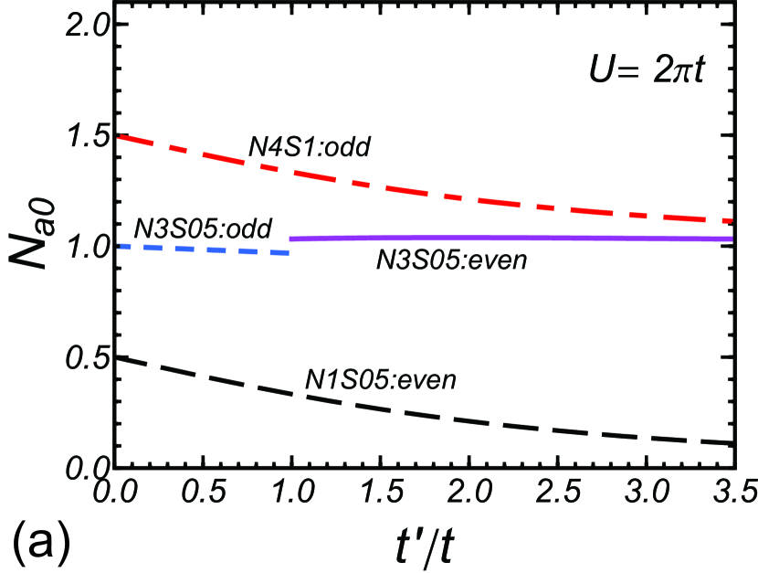
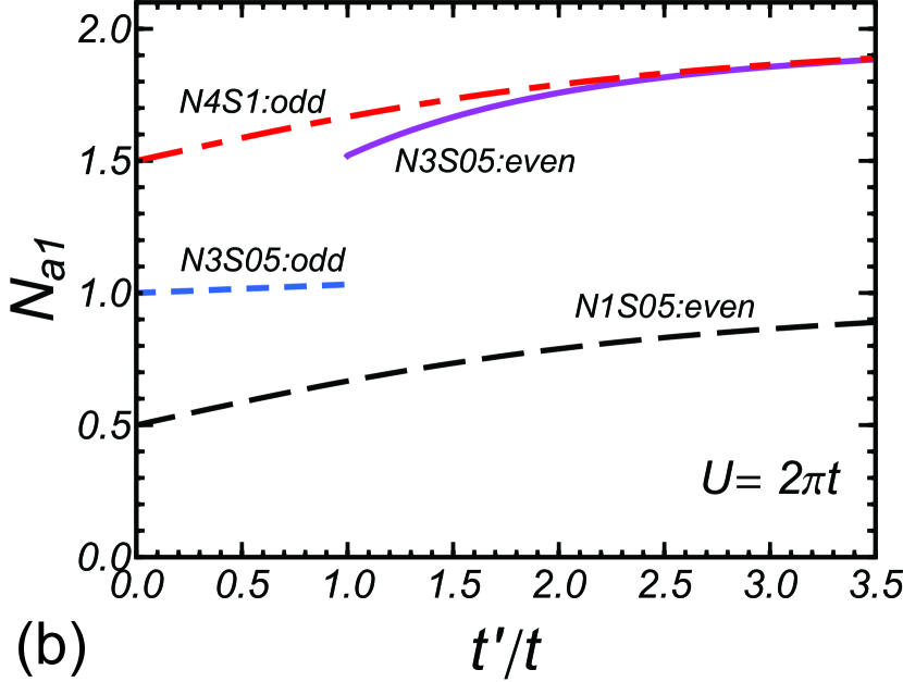
Figure 16: (Color online) Charge distribution in the isolated TTQD, $N_{a,i}\equiv\sum_{\sigma}\langle n_{a,i\sigma}\rangle$ is plotted as a function of $t^{\prime}/t$ for (a) $N_{a0}$ the apex site, and for (b) the even $a_{1}$ orbital described in Appendix B. The average is taken with respect to some of the eigenstates of $\mathcal{H}_{\mathrm{dot}}\equiv\mathcal{H}_{\mathrm{dot}}^{0}+\mathcal{H}_{\mathrm{dot}}^{U}$, and labelled by the occupation number, spin, and parity (“N3S05:even” denotes, “$N_{\mathrm{tot}}=3$”, $S=1/2$, and an even parity). The parameters are chosen to be $\Gamma=0$, $U/(2\pi t)=1.0$, and $\epsilon_{\mathrm{apex}}=\epsilon_{d}$. Note that the occupation number takes the form $N_{\mathrm{tot}}=N_{a,0}+N_{a,1}+N_{b,1}$.

The results for $T^{*}$ are plotted in Fig.  15 using a logarithmic scale, as a function of $\epsilon_{d}/U$ and $t^{\prime}/t$ for $\Gamma/t=0.25$ and $U/(2\pi t)=1.0$. The phase diagram of the isolated TTQD given in Fig. 5 (b) is also superposed onto Fig.  15 with the dashed lines, as a guide for the eye. We can see that the variation of $T^{*}$ in the parameter space also relates to the plateaus of $\Theta$ [see Fig. 11 in Appendix B]. The energy scale $T^{*}$ is large in the case that the quantum dots have no local moment, and it becomes smaller when the TTQD has a local moment.

We can see, nevertheless, $T^{*}$ is still relatively high in the regions of $N_{\mathrm{tot}}\simeq 1.0$ and $5.0$, in which the $S=1/2$ Kondo effect takes place. The $S=1/2$ moment for $N_{\mathrm{tot}}\simeq 1.0$ is caused by a single electron, which enters an even-parity state and stays mainly at the $a_{1}$ orbital adjacent to the leads [see Fig. 21]. Thus the screening can be completed relatively easily in this case. Figure 16 shows the occupation number $N_{a0}$ ($N_{a1}$) in the $a_{0}$ ($a_{1}$) orbital, as a function of $t^{\prime}/t$, for the limit of $\Gamma\to 0$: note that $a_{0}$ corresponds to the apex site. The dashed line which is labelled “N1S05:even” shows the average with respect to the lowest eigenvector in the subspace with $N_{\mathrm{tot}}=1$, $S=1/2$, and an even parity. We can see that $N_{a1}$ approaches to $1.0$ as $t^{\prime}/t$ increases. In the opposite case, at $t^{\prime}/t=0.0$, the occupation number for $a_{0}$ and that for $a_{1}$ coincide $N_{a0}=N_{a1}=0.5$, but still the charge and spin fluctuations are not suppressed because these orbitals are still at quarter filling.

In the five-electron region for $t^{\prime}/t>1.0$, the eigenvector $|\Phi^{(5)}_{\mathrm{odd}}\rangle$ for the isolated TTQD can be expressed in the form of Eq. (37). The local moment in this case stays at the $b_{1}$ orbital, which is also adjacent to one of the leads [see Fig. 21], and the conduction electrons can screen the moment through the usual kinetic exchange mechanism. For another five-electron region at $0\leq t^{\prime}/t<1.0$, the eigenvector $|\Phi^{(5)}_{\mathrm{even}}\rangle$ can be written in the form of Eq. (36). The averages $N_{a0}$ and $N_{a1}$ with respect to this state coincide with those with respect to the Nagaoka state $|\Phi^{(4)}_{\mathrm{odd}}\rangle$ defined in Eq. (35), and the results are plotted in Fig. 16 with the dot-dash line labelled “N4S1:odd”. We can see that for $0\leq t^{\prime}/t<1.0$ a single hole with a spin $1/2$ enters both of the even orbitals, and for $t^{\prime}/t\to 0$ these orbitals approach to quarter filling in the hole picture. Therefore, the screening is not suppressed so much also in this five-electron region.

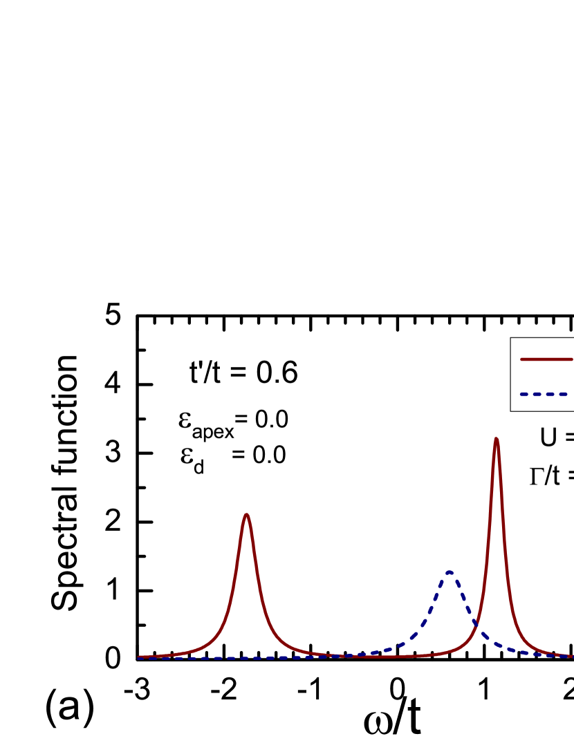
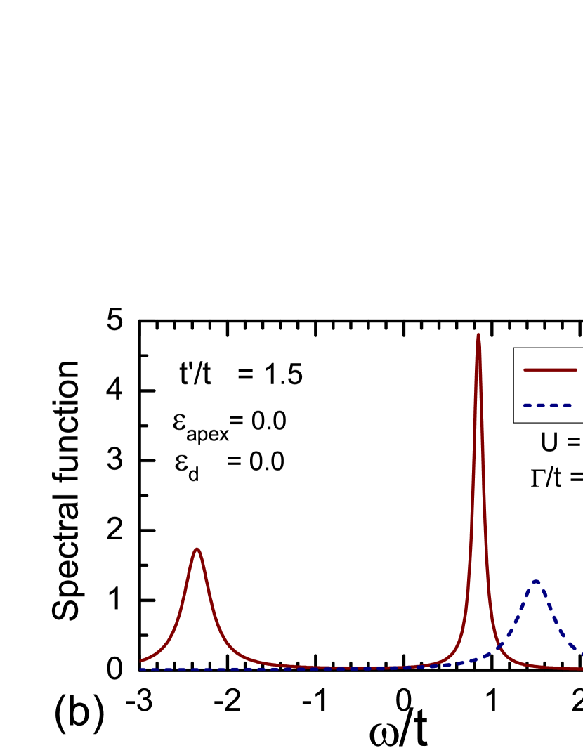
Figure 17: (Color online) Spectral functions in the noninteracting case for (a) $t^{\prime}/t=0.6$ and (b) $t^{\prime}/t=1.5$. The solid line is the even component $-\mathrm{Im}\,[G_{a0}(\omega)+G_{a1}(\omega)]/\pi$, and the dotted line is the odd component $-\mathrm{Im}\,G_{b0}(\omega)/\pi$, defined in Appendix B. The other parameters are chosen to be $\Delta\epsilon=0.0$, $\epsilon_{d}=0.0$, and $\Gamma/t=0.25$.

The screening temperature becomes small in the three and four electron regions, namely $-1.1\lesssim\epsilon_{d}\lesssim-0.3$ in Fig.  15. We can see in the three electron region, however, $T^{*}$ is still much higher for $t^{\prime}/t\lesssim 1.0$ than for $t^{\prime}/t\gtrsim 1.0$ despite the local moment in the TTQD is $S=1/2$ in both of the cases. For $t^{\prime}/t\lesssim 1.0$, the ground state is an odd-parity state, and one of the three electrons enters the $b_{1}$ orbital, and the other two electrons enter almost equally to the $a_{0}$ and $a_{1}$ orbitals. This can be confirmed through the dotted line labelled “N3S05:odd” in Fig. 16. We can also see in Fig. 17 (a) that the third electron enters the odd $b_{1}$ orbital for $t^{\prime}/t\lesssim 1.0$ in the noninteracting limit. In contrast, for $t^{\prime}/t\gtrsim 1.0$ the ground state is an even parity state, and the solid line labelled “N3S05:even” denotes average with respect to this state. We see that $N_{a1}$ approaches to $2.0$ as $t^{\prime}/t$ increases, while the occupation of the apex site is almost unchanged $N_{a0}\simeq 1.0$, and thus the occupation of the $b_{1}$ orbital is decreasing in this case. Therefore, the local moment is mainly due to the electron staying at the apex site. Thus the screening is protracted significantly because the charge and spin fluctuations are suppressed at the nearly filled $a_{1}$ orbital, over which the conduction electrons come to screen the moment. We have also confirmed that along the sharp conductance valley caused by the SU(4) Kondo effect, at $t^{\prime}/t\simeq 1.0$ and $-0.8\lesssim\epsilon_{d}/U\lesssim-0.3$, the energy scale $T^{*}$ is enhanced due to the orbital degeneracy. Note that the variations in the spin and charge configurations near the SU(4) symmetric point becomes wider in the TTQD than the double dot.

The properties of the local moment in the three-electron region also reflect the feature of the one-particle state which emerges as a peak of the conductances shown in Fig.  3, and also the corresponding spectral function is shown in Fig. 17. Specifically for $t^{\prime}/t\gtrsim 1.0$ the orbital degeneracy is lifted such that $E_{\mathrm{o}}^{(1)}>E_{\mathrm{e,+}}^{(1)}$. Therefore, after two electrons occupy the lowest even-parity orbital with the energy $E_{\mathrm{e,-}}^{(1)}$, the third electron enters the resonance state corresponding to the excited even-parity orbital which appears in Fig. 17 (b) as the central peak. This state has a dominant spectral weight in the apex site, and the resonance width is narrower than $\Gamma$ already in the noninteracting case [see also Eq. (31) in Appendix B]. It should also be noted that the width of this resonance determines $T^{*}$ in the noninteracting limit. For finite $U$, this peak may evolve into a Kondo resonance whose width is reduced further by the Coulomb interaction to the value of the order of $\,T^{*}$.

The wavefunction for the Nagaoka state has an odd parity, and the charge distribution of this state is shown in Fig. 16, with the dot-dash line labelled “N4S1:odd”. We can see that $N_{a0}$ and $N_{a1}$ for the Nagaoka state are similar to those for the three electrons state “N3S05:even”. The fraction of the local moment stays at the apex site, and this explains the reason why $T^{*}$ is small also in this case. One extra electron enters mainly the $b_{1}$ orbital, and it provides half of the $S=1$ moment which can be screened at high temperature at the first stage of the two-stage Kondo screening.Numata2

Figure 18: (Color online) The characteristic energy scale $T^{*}$ in the $\epsilon_{d}/U$ vs $\Delta\epsilon/U$ plane for $\Gamma/t=0.12$, $U/(2\pi t)=1.0$, and $t^{\prime}=t$. The results in the range of $-30<\log_{10}(T^{*}/\Gamma)<0$ are painted in the colors varying from blue to red. $T^{*}$ becomes very small in the purple region, and the solid lines there denote the contours for $\log_{10}(T^{*}/\Gamma)=-30,\,-60$, and $-90$. The dashed lines denote the phase boundary in the limit of $\Gamma\to 0$, corresponding to Fig. 6 (b).

VI.2 $T^{*}$ vs diagonal distortions ($\epsilon_{\mathrm{apex}}\neq\epsilon_{d}$)

The characteristic energy scale $T^{*}$ for the TTQD with the diagonal distortions is plotted in Fig.  18 using a logarithmic scale, as a function of $\epsilon_{d}/U$ and $\Delta\epsilon/U$ for $U/(2\pi t)=1.0$. The phase diagram of the isolated TTQD given in Fig. 6 (b) is also superposed onto Fig.  18. Note that the coupling between the leads and quantum dots is chosen to be $\Gamma/t=0.12$, which is smaller than that we chose for the off-diagonal case. Therefore, the absolute values of $T^{*}$ become smaller than those in Fig. 15. We saw in the above that the Kondo screening is sensitive to the electronic structure of the TTQD for the off-diagonal distortions $t^{\prime}\neq t$. In order to see the results in a similar way, the charge distribution in the even and odd orbitals in the isolated TTQD for $\Gamma\to 0$ is also plotted in Fig. 19 as a function $\Delta\epsilon$ ($\equiv\epsilon_{\mathrm{apex}}-\epsilon_{d}$).

We can see that $T^{*}$ is suppressed also in the region of $N_{\mathrm{tot}}\simeq 1.0$ at $\Delta\epsilon\lesssim 0.0$, which corresponds to the area of $\epsilon_{d}/U\gtrsim 0.3$ at the right bottom of Fig.  18. In this parameter region, the potential profile of the onsite energy is such that $\epsilon_{\mathrm{apex}}<E_{F}$ and $\epsilon_{d}>E_{F}$, with the Fermi energy $E_{F}\equiv 0.0$. Therefore, the single electron enters mainly the apex site, and the other two dots are almost empty. This can also be confirmed through the charge distribution plotted with the dashed line labelled “N1S05:even” in Fig. 19. For $\Delta\epsilon\lesssim 0.0$, the occupation number $N_{a0}$ for the apex site approaches to $1.0$ while that for the even $a_{1}$ orbital, $N_{a1}$, almost vanishes. Therefore, the screening of the local moment is achieved through a super-exchange process by the conduction electrons which come to the apex site over the potential barrier at the other two dots, and thus $T^{*}$ decreases in this parameter region.

Similarly, $T^{*}$ is suppressed also in the five-electron region for $\Delta\epsilon>0.0$, which corresponds to the area for $\epsilon_{d}/U\lesssim-1.2$ at the top left of Fig.  18. The ground state in this parameter region has an even parity, and in the limit of $\Gamma\to 0$ the eigenvector is given by $|\Phi^{(5)}_{\mathrm{even}}\rangle$ in Eq. (36). The average number of electrons $N_{a0}$ and $N_{a1}$ for this state coincide with those with respect to $|\Phi^{(4)}_{\mathrm{odd}}\rangle$ defined in Eq. (35). The results are shown in Fig. 19, with the dot-dash line labelled “N4S1:odd”. We can see that a single hole with a spin $1/2$ stays in the apex site for $\Delta\epsilon\gtrsim 0.0$, and the other two dots are almost doubly occupied. Therefore, $T^{*}$ becomes very small in this case. This can also understood from the feature of the spectral function, shown in Fig. 20. The Fermi level for the five electrons in this case is situated in the middle of the sharp peak at $\omega\simeq 1.2t$ in Fig. 20 (a). The width of this resonance corresponds to $T^{*}$ in the noninteracting limit, and the peak will become much narrower for finite Coulomb interaction $U$. There is another five-electron region for $\Delta<0.0$, where the eigenvector is given by $|\Phi^{(5)}_{\mathrm{odd}}\rangle$ in Eq. (37) for the isolated TTQD. The local moment in this case stays at the $b_{1}$ orbital, which is close to one of the leads, and thus the screening can be achieved by the usual kinetic exchange mechanism of the $S=1/2$ Kondo effect.

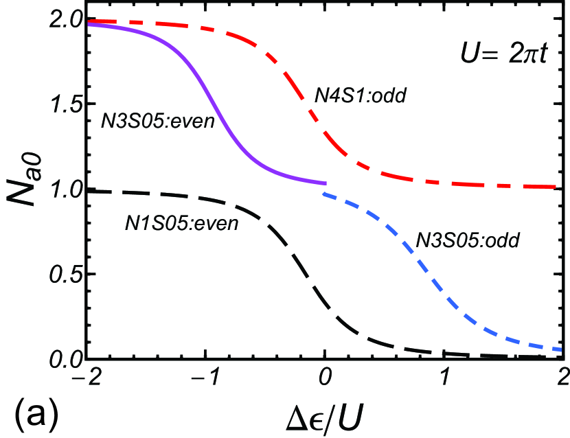
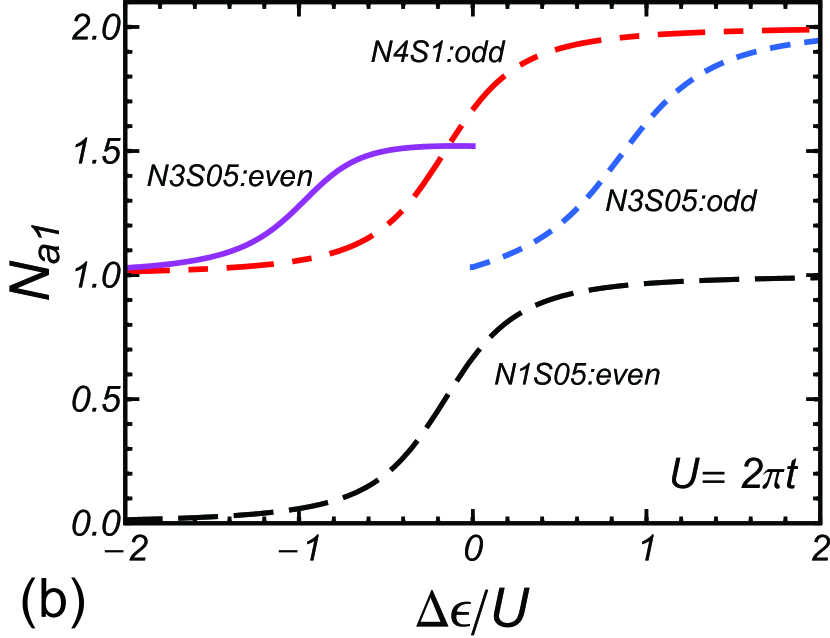
Figure 19: (Color online) Charge distribution in the isolated TTQD, $N_{a,i}\equiv\sum_{\sigma}\langle n_{a,i\sigma}\rangle$, is plotted as a function of $\Delta\epsilon/U$ for (a) $N_{a0}$ the apex site, and for (b) the even $a_{1}$ orbital described in Appendix B. The average is taken with respect to some of the eigenstates of $\mathcal{H}_{\mathrm{dot}}\equiv\mathcal{H}_{\mathrm{dot}}^{0}+\mathcal{H}_{\mathrm{dot}}^{U}$, and labelled by the occupation number, spin, and parity (“N4S1:odd” denotes, $N_{\mathrm{tot}}=4$, $S=1$, and an odd parity). The parameters are chosen to be $\Gamma=0$, $U/(2\pi t)=1.0$, and $t^{\prime}=t$. Note that $\Delta\epsilon\equiv\epsilon_{\mathrm{apex}}-\epsilon_{d}$, and the occupation number takes the form $N_{\mathrm{tot}}=N_{a,0}+N_{a,1}+N_{b,1}$,

The screening temperature becomes small also in the three region, and in the four electron region. In the three electron region for $\Delta\epsilon\gtrsim 0.0$ the ground state has an odd parity, and the charge distribution for this state is plotted in Fig. 19, with the dotted line labelled “N3S05:odd”. We can see that at $\Delta\epsilon\simeq 1.0$ the three electrons distribute almost homogeneously as $N_{a0}\simeq N_{a1}\simeq 1.0$, and thus $N_{b1}\simeq 1.0$. Then, as $\Delta\epsilon$ increases, a single electron in the apex site moves towards the even-parity $a_{1}$ orbital, and the occupation numbers approach to $N_{a0}\simeq 0.0$ and $N_{a1}\simeq 2.0$, keeping the occupation of the odd-parity orbital almost unchanged $N_{b1}\simeq 1.0$. Therefore, $T^{*}$ becomes larger as $\Delta\epsilon$ increases.

The ground state in the other three electron region, for $\Delta\epsilon\lesssim 0.0$, has an even parity. The charge distribution with respect to this state is shown with the solid line labelled “N3S05:even” in Fig. 19, and in this case it is such that $N_{a0}\simeq 1.0$, $N_{a1}\simeq 1.5$, and $N_{b1}\simeq 0.5$ near $\Delta\epsilon\simeq 0.0^{-}$. Therefore, the apex site is singly occupied, and the moment protracted. The distribution varies as $\Delta\epsilon$ decreases, and the fraction of the local moment tends to stay close to the leads, as $N_{a0}\simeq 2.0$, $N_{a1}\simeq 0.5$, and $N_{b1}\simeq 0.5$. We have also confirmed that $T^{*}$ is enhanced near $\Delta\epsilon\simeq 0.0$ and $-0.7\lesssim\epsilon_{d}/U\lesssim-0.4$, along the sharp conductance valley caused by the SU(4) Kondo effect. The local moment in the three-electron region also reflects the properties of the one-particle state. Similar to the $t^{\prime}/t\gtrsim 1.0$ case discussed in the previous subsection, the orbital degeneracy is lifted as $E_{\mathrm{o}}^{(1)}>E_{\mathrm{e,+}}^{(1)}$ for $\Delta\epsilon\lesssim 0.0$. In this case the third electron enters the resonance state corresponding to the excited even-parity orbital, appearing in the middle of Fig. 20 (b). Since the spectral weight of this state is mainly at the apex site, the resonance width becomes narrow already in the noninteracting case and it evolves into a sharp Kondo resonance for finite $U$.

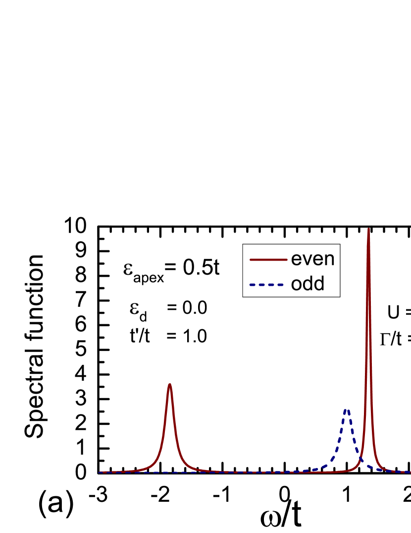
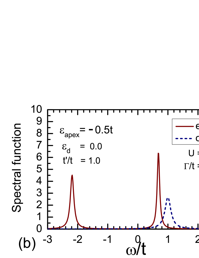
Figure 20: (Color online) Spectral functions in the noninteracting case for (a) $\Delta\epsilon=0.5t$ and (b) $\Delta\epsilon=-0.5t$. The solid line is the even component $-\mathrm{Im}\,[G_{a0}(\omega)+G_{a1}(\omega)]/\pi$, and the dotted line is the odd component $-\mathrm{Im}\,G_{b0}(\omega)/\pi$, defined in Appendix B. The other parameters are chosen to be $t^{\prime}/t=1.0$, $\epsilon_{d}=0.0$, and $\Gamma/t=0.12$.

The $S=1$ Kondo effect takes place in the four electron region at $-0.4\lesssim\Delta\epsilon/U\lesssim 0.8$ in Fig.  18. We can see that $T^{*}$ varies significantly inside this region depending on whether $\Delta\epsilon\lesssim 0.0$ or $\Delta\epsilon\gtrsim 0.0$, although the $S=1$ Nagaoka high-spin state which has an odd parity evolves continuously as $\Delta\epsilon$ varies. The eigenvector in the limit of $\Gamma\to 0$ is given by $|\Phi^{(4)}_{\mathrm{odd}}\rangle$, and the charge distribution with respect to this state is shown in Fig. 19, with the dot-dash line labelled “N4S1:odd”. We can see that $N_{a0}$ and $N_{a1}$ vary rapidly near $\Delta\epsilon\simeq 0.0$, keeping the filling of $b_{1}$ orbital unchanged $N_{b1}=1.0$. For $\Delta\epsilon\gtrsim 0.0$, the local moment has a finite component in the apex site. This component of the moment moves to the $a_{1}$ orbital near the leads for $\Delta\epsilon\lesssim 0.0$. The variation of $T^{*}$ inside the $S=1$ Kondo region reflects these changes in the charge and spin distributions.

VII Summary

We have studied the effects of distortions which break the full symmetry of an equilateral triangle of a TTQD connected to two non-interacting leads, over a wide range of the gate voltage $\epsilon_{d}$. Two types of disorder have been considered, ($i$) an inter-dot tunneling matrix element $t^{\prime}$ ($\neq t$), and ($ii$) a level position $\epsilon_{\mathrm{apex}}$ ($\neq\epsilon_{d}$) of the dot at the apex site. We have concentrated on the low energy behavior, restricting attention mainly to the regime with large Coulomb interaction $U$ and small hybridization $\Gamma$ as this leads to several different types of the Kondo effect.

We find that the key variables for characterizing the low energy behavior are the total occupation number $N_{\mathrm{tot}}$ and the phase difference $\Theta\equiv(\delta_{\mathrm{e}}-\delta_{\mathrm{o}})(2/\pi)$. The two phase shifts for the renormalized quasi-particles, $\delta_{\mathrm{e}}$ and $\delta_{\mathrm{o}}$, can be deduced theoretically from the low energy NRG fixed point. The phase shifts may be deduced experimentally through the conductances and $N_{\mathrm{tot}}$. Measurements of the AB oscillation in a magnetic field may also give a clue to determine the phase difference.

In the parameter space for large $U$ we find plateaus with the integer values of $\Theta$, and at each plateau the occupation number also approaches to an integer. These plateaus, therefore, can be classified with the two integer set $(N_{\mathrm{tot}},\Theta)$ [see Figs. 11 and 14]. The structure of these plateaus of $\Theta$ determines the precise feature of the Kondo ridges and valleys of the conductance [see Figs. 8 and 13].

Different Kondo effects occur in different regimes. The SU(4) Kondo effect takes place for weak distortions, along the contour line for $\Theta=2.0$ which runs in the region of $N_{\mathrm{tot}}\simeq 3.0$ in the parameter space. This contour transverses the middle of a steep cliff of $\Theta$, standing between the plateau for $\Theta\simeq 1.0$ and that for $\Theta\simeq 3.0$. It can be observed as a sharp conductance valley between the Kondo ridges on both sides, and the slope of the cliff determines the width of the conductance valley. The SU(4) Kondo behavior is sensitive to the perturbations which lower the symmetry of the equilateral triangle. This is caused by the fact that the SU(4) symmetry relies crucially on the orbital degeneracy. Furthermore, the spin and charge distributions inside the TTQD vary near the SU(4) symmetric point, and it affects significantly the Kondo screening.

The $S=1$ Kondo effect, taking place at the plateau of $\Theta$ for $(N_{\mathrm{tot}},\Theta)\simeq(4.0,\,2.0)$, is robust against the breaking of the symmetry of the equilateral triangle. This is mainly due to a size effect: there is a finite energy separation between the Nagaoka high-spin state and the excited local singlet state in the isolated TTQD cluster. For large distortions a singlet-triplet transition takes place. It becomes a crossover between a Kondo and non-Kondo singlet state for finite $\Gamma$, and the series conductance has a peak of the height of $2e^{2}/h$ in the transient regions. The width of the peak is determined by the slope of the cliff of $\Theta$, which appears at the crossover region.

Apart from the phase shifts which determine the conductance and occupation of the TTQD, another important renormalized parameter characterizing the low energy behavior is the characteristic energy scale $T^{*}$. For $T\lesssim T^{*}$ the low-energy properties can be described by the local Fermi-liquid theory. In the cases where the quantum dots have a local moment, $T^{*}$ can be regarded as the Kondo temperature. We have estimated $T^{*}$ from the region where the NRG levels crossover to the low energy fixed point. The results for $T^{*}$ reflect the distribution of the charge and spin in the TTQD [Figs. 15 and 18].

Specifically, $T^{*}$ tends to be small in the case where a partial moment remains in the apex site, which has no direct coupling to the leads. The screening of such a partial moment becomes sensitive to the charge and spin on the other two dots because the conduction electrons tunneling from the leads have to pass through either of the two dots to get the apex site. In some regions of the parameter space, we find that the tunneling of the conduction electron is suppressed at these two dots, in a way analogous to a super-exchange process caused by a potential barrier between the local moment and leads. The characteristic temperature $T^{*}$ can be raised, however, by making the coupling to the leads $\Gamma$ stronger. Note that $T^{*}$ depends on $\Gamma$ not only through the prefactor, but also through the higher order contributions of the hybridization, which cause an exponential dependence of $T^{*}$ on $\Gamma$ and other parameters. Specifically, $T^{*}$ may become large for the TTQD with a small charging energy $U$. Our results provide an overview of how characteristic energy scale varies in the different the regions in the parameter space.

A general point worthy of note is that the two types of the distortions show a clear contrast in the form of the charge distribution for some regions of the parameter space [see Figs.  16 and 19]. The diagonal distortion ($\epsilon_{\mathrm{apex}}\neq\epsilon_{d}$) affects directly the potential of the apex site, so that the charge distribution is more sensitive to $\Delta\epsilon$ than to the off-diagonal one ($t^{\prime}\neq t$), and this difference affects the characteristic energy scale $T^{*}$ significantly in some regions of the parameter space.

Appendix A Phase shifts $\delta_{\mathrm{e}}$ and $\delta_{\mathrm{o}}$

The phase shifts for interacting electrons can be defined, using the Green’s function

$$G_{ij}(i\omega_{n})\,=\,-\int_{0}^{\beta}\!d\tau\,\left\langle T_{\tau}\,d^{\phantom{\dagger}}_{i\sigma}(\tau)\,d^{\dagger}_{j\sigma}(0)\right\rangle\,e^{i\omega_{n}\tau}\;.$$ (18)

Here, $\beta=1/T$, $d_{j\sigma}(\tau)=e^{\tau{\cal H}}d_{j\sigma}e^{-\tau{\cal H}}$, and $\langle{\cal O}\rangle=\mbox{Tr}\left[\,e^{-\beta{\cal H}}\,{\cal O}\,\right]/\mbox{Tr}\,e^{-\beta{\cal H}}$. The retarded Green’s function is given by $G_{ij}^{+}(\omega)\equiv G_{ij}(\omega+i\,0^{+})$ via the analytic continuation, and the self energy $\Sigma_{ij}(z)$ due to the interaction $\mathcal{H}_{\mathrm{dot}}^{U}$ can be described by the Dyson equation

$$G_{ij}(z)=G^{(0)}_{ij}(z)+\sum_{i^{\prime}=1}^{N_{D}}\sum_{j^{\prime}=1}^{N_{D}}\,G^{(0)}_{ii^{\prime}}(z)\,\Sigma_{i^{\prime}j^{\prime}}(z)\,G_{j^{\prime}j}(z)\;.$$ (19)

Here, the number of the dots is $N_{D}=3$ for the TTQD, and $G^{(0)}_{ij}(z)$ is the non-interacting Green’s function corresponding to the free Hamiltonian $\mathcal{H}_{0}\equiv\mathcal{H}_{\mathrm{dot}}^{0}+\mathcal{H}_{\mathrm{mix}}+\mathcal{H}_{\mathrm{lead}}$.

At zero temperature $T=0$, the series $g_{\mathrm{s}}$ and parallel $g_{\mathrm{p}}$ conductances are determined by the Green’s functions at the Fermi level $\omega=0$,aoQuasi ; ONH

$$g_{\mathrm{s}}^{\phantom{0}}\,= \ \frac{2e^{2}}{h}4\Gamma_{R}\Gamma_{L}\left|G_{N_{D}1}^{+}(0)\right|^{2}\;,$$ (20)

$$g_{\mathrm{p}}^{\phantom{0}}= \ {2e^{2}\over h}\,\Bigl{[}\,-\Gamma_{L}\,\mathrm{Im}\,G_{11}^{+}(0)-\Gamma_{R}\,\mathrm{Im}\,G_{N_{D}N_{D}}^{+}(0)\,\Bigr{]}\;.$$ (21)

Note that the contributions from the vertex correction do not appear here due to the property that the imaginary part of the self-energy vanishes $\mathrm{Im}\,\Sigma_{ij}^{\pm}(0)=0$ at $T=0$ and $\omega=0$.aoFermi Furthermore, for the symmetric coupling $\Gamma_{L}=\Gamma_{R}$ ($\equiv\Gamma$), the Green’s functions can be expressed in the forms,

$$G_{11}^{+}(0)=G_{N_{D}N_{D}}^{+}(0)\,= \ \frac{1}{2\Gamma}\left[\,\frac{1}{\kappa_{\mathrm{e}}+{i}}\,+\,\frac{1}{\kappa_{\mathrm{o}}+i}\,\right]\;,$$ (22)

$$G_{N_{D}1}^{+}(0)\,= \ \frac{1}{2\Gamma}\left[\,\frac{1}{\kappa_{\mathrm{e}}+i}\,-\,\frac{1}{\kappa_{\mathrm{o}}+i}\,\right]\;.$$ (23)

Here, $\kappa_{\mathrm{e}}=-\cot\delta_{\mathrm{e}}$ and $\kappa_{\mathrm{o}}=-\cot\delta_{\mathrm{o}}$ include all the many-body corrections, through the real part of the self-energy $\mathrm{Re}\,\Sigma_{ij}^{+}(0)$.ONH Equations (6)–(8) follow from Eqs. (20)–(23).

Figure 21: Even and odd orbitals: the onsite potential of each orbital is given by $\,\epsilon_{a0}=\epsilon_{\mathrm{apex}}$, $\,\epsilon_{a1}=\epsilon_{d}-t^{\prime}$, and $\,\epsilon_{b1}=\epsilon_{d}+t^{\prime}$.

Appendix B Even and odd orbitals

The eigenstates of the Hamiltonian $\mathcal{H}$ defined in Eq. (1) can be classified according to the parity in the case that the system has an inversion symmetry, using the even-odd basis defined by $a_{0\sigma}\equiv d_{2\sigma}$,

$$a_{1\sigma}\equiv\frac{d_{1\sigma}+\,d_{3\sigma}}{\sqrt{2}}\;,\qquad\quad b_{1\sigma}\equiv\frac{d_{1\sigma}-\,d_{3\sigma}}{\sqrt{2}}\;.$$ (24)

The labels $0$ and $1$ for the even-odd basis are assigned in the way that is shown in Fig. 21. The odd parity $b_{1}$ orbital corresponds to the eigenstate for $E_{\mathrm{o}}^{(1)}$, defined in Eq. (15), for the noninteracting TTQD cluster. Similarly the eigenstate for $E_{\mathrm{e,\pm}}^{(1)}$ is given by a linear combination of the even $a_{0}$ and $a_{1}$ orbitals.

$$|\Phi^{(1)}_{\mathrm{e,+}}\rangle\,= \ \left(u_{+}\,a^{\dagger}_{0\sigma}\,+\,u_{-}\,a^{\dagger}_{1\sigma}\right)|0\rangle,$$ (25)

$$|\Phi^{(1)}_{\mathrm{e,-}}\rangle\,= \ \left(-u_{-}\,a^{\dagger}_{0\sigma}\,+\,u_{+}\,a^{\dagger}_{1\sigma}\right)|0\rangle\;.$$ (26)

Here, $|0\rangle$ is a vacuum. The coefficients are normalized such that $u_{+}^{2}+u_{-}^{2}=1$,

$$u_{\pm}^{2}= \ \frac{1}{2}\left(1\pm\frac{\Delta\epsilon+t^{\prime}}{\sqrt{(\Delta\epsilon+t^{\prime})^{2}+8t^{2}}}\right)$$ (27)

and $u_{+}^{2}$ ($u_{-}^{2}$) corresponds to the spectral weight for the $a_{0}$ ($a_{1}$) component in the excited state $|\Phi^{(1)}_{\mathrm{e,+}}\rangle$. When the TTQD is coupled to the leads, these states become the resonance levels, which can be described by the Green’s functions for the $a_{0}$, $a_{1}$, and $b_{1}$ orbitals

$$G_{a0}^{(0)}(\omega)= \ \frac{1}{\omega-\epsilon_{\mathrm{apex}}-\frac{2t^{2}}{\omega-\epsilon_{d}+t^{\prime}+i\Gamma}}\;,$$ (28)

$$G_{a1}^{(0)}(\omega)= \ \frac{1}{\omega-\epsilon_{d}+t^{\prime}+i\Gamma-\frac{2t^{2}}{\omega-\epsilon_{\mathrm{apex}}}}\;,$$ (29)

$$G_{b1}^{(0)}(\omega)= \ \frac{1}{\omega-\epsilon_{d}-t^{\prime}+i\Gamma}\;.$$ (30)

Specifically for $\Delta\epsilon+t^{\prime}>0$ the coefficients take the value of $u_{+}^{2}>0.5$ and $u_{-}^{2}<0.5$. In this case the even excited state $|\Phi^{(1)}_{\mathrm{e,+}}\rangle$ becomes a sharp resonance peak, the spectral weight of which is mainly on the apex site, and the spectral function near $\omega\simeq E_{\mathrm{e,+}}^{(1)}$ takes the form

$$-\mathrm{Im}\,G_{a0}^{(0)}(\omega)\ \simeq \ \ u_{+}^{2}\,\frac{u_{-}^{2}\Gamma}{\left(\omega-E_{\mathrm{e,+}}^{(1)}\right)^{2}+\left(u_{-}^{2}\Gamma\right)^{2}}\;,$$ (31)

$$-\mathrm{Im}\,G_{a1}^{(0)}(\omega)\ \simeq \ \ u_{-}^{2}\,\frac{u_{-}^{2}\Gamma}{\left(\omega-E_{\mathrm{e,+}}^{(1)}\right)^{2}+\left(u_{-}^{2}\Gamma\right)^{2}}\;.$$ (32)

The Green’s functions near the lower level $\omega\simeq E_{\mathrm{e,-}}^{(1)}$ can also be written in similar forms, just by replacing $+$ ($-$) in the suffix by $-$ ($+$) in Eqs. (31) and (32).

The interaction Hamiltonian defined in Eq. (3) can be expressed, in terms of these even-odd orbitals, in the form

$$\mathcal{H}_{\mathrm{dot}}^{U}= \ Un_{a,0\uparrow}\,n_{a,0\downarrow}+\frac{U}{2}\left(n_{a,1\uparrow}\,n_{a,1\downarrow}+n_{b,1\uparrow}\,n_{b,1\downarrow}\right)$$

$$+\frac{U}{2}\left(\frac{1}{2}n_{a,1}\,n_{b,1}-2\vec{\bm{S}}_{a,1}\cdot\vec{\bm{S}}_{b,1}\right)$$

$$+\frac{U}{2}\left(a^{\dagger}_{1\uparrow}a^{\dagger}_{1\downarrow}b_{1\downarrow}b_{1\uparrow}+b^{\dagger}_{1\uparrow}b^{\dagger}_{1\downarrow}a_{1\downarrow}a_{1\uparrow}\right).$$ (33)

Here, $\vec{\bm{S}}_{a,i}=\sum_{\sigma\sigma^{\prime}}a^{\dagger}_{i\sigma}\vec{\bm{\sigma}}_{\sigma\sigma^{\prime}}a_{i\sigma^{\prime}}/2$, $\,\,\vec{\bm{\sigma}}$ the Pauli matrices, $n_{a,i\sigma}=a^{\dagger}_{i\sigma}a_{i\sigma}$, and $n_{a,i}=\sum_{\sigma}n_{a,i\sigma}$. The operators $n_{b,1\sigma}$ and $\vec{\bm{S}}_{b,1}$ for the odd-parity orbital $b_{1\sigma}$ are defined in the same way.

The Hilbert space for the isolated TTQD cluster, described by $\mathcal{H}_{\mathrm{dot}}=\mathcal{H}_{\mathrm{dot}}^{0}+\mathcal{H}_{\mathrm{dot}}^{U}$, can be constructed from the three orbitals. For instance, the Nagaoka state for $\mathcal{H}_{\mathrm{dot}}$ has an odd parity. It has one electron in the $b_{1}$ orbital, and the eigenvector takes the form

$$|\Phi^{(4)}_{\mathrm{odd}}\rangle=\ \alpha_{0}\,|\mathrm{I}\rangle+\alpha_{1}\,|\mathrm{II}\rangle\;,$$ (34)

$$\ \ |\mathrm{I}\rangle=b^{\dagger}_{1\uparrow}a^{\dagger}_{1\uparrow}a^{\dagger}_{0\uparrow}a^{\dagger}_{0\downarrow}|0\rangle,\quad|\mathrm{II}\rangle=b^{\dagger}_{1\uparrow}a^{\dagger}_{1\uparrow}a^{\dagger}_{1\downarrow}a^{\dagger}_{0\uparrow}|0\rangle\;.$$ (35)

Here, $\alpha_{0}$ and $\alpha_{1}$ are the coefficients. The eigenvectors for five electrons can be expressed in the form

$$|\Phi^{(5)}_{\mathrm{even}}\rangle=\,b^{\dagger}_{1\downarrow}|\Phi^{(4)}_{\mathrm{odd}}\rangle\;,$$ (36)

$$|\Phi^{(5)}_{\mathrm{odd}}\rangle=\,b^{\dagger}_{1\uparrow}a^{\dagger}_{1\uparrow}a^{\dagger}_{1\downarrow}a^{\dagger}_{0\uparrow}a^{\dagger}_{0\downarrow}|0\rangle.$$ (37)

Therefore, the odd-parity $b_{1}$ orbital is fully occupied for $|\Phi^{(5)}_{\mathrm{even}}\rangle$, while the even $a_{0}$ and $a_{1}$ orbitals are fully occupied for $|\Phi^{(5)}_{\mathrm{odd}}\rangle$. The distribution of the charge and spin in the three orbitals affects significantly on the way the screening by the conduction electrons is carried out for finite $\Gamma$, when the leads are connected to the TTQD.

Appendix C NRG approach

We provide an explicit form of the discretized Hamiltonian $H_{N}$ of the NRG in this appendix. The non-interacting leads are transformed into the tight-biding chains in the NRG approach, through the logarithmic discretization with the parameter $\Lambda$. Then, a sequence of the Hamiltonian $H_{N}$ with a finite size is introduced in the formKWW ; KWW2

$$H_{N}\ =\Lambda^{(N-1)/2}\left(\mathcal{H}_{\mathrm{dot}}^{0}+\mathcal{H}_{\mathrm{dot}}^{U}+H_{\mathrm{mix}}^{\phantom{0}}+H_{\mathrm{lead}}^{(N)}\right),$$ (38)

$$H_{\mathrm{mix}}^{\phantom{0}}\,=\,\bar{v}\,\sum_{\sigma}\left(\,f^{\dagger}_{0,L\sigma}d^{\phantom{\dagger}}_{1,\sigma}\,+\,d^{\dagger}_{1,\sigma}f^{\phantom{\dagger}}_{0,L\sigma}\right)$$

$$\qquad\quad+\bar{v}\,\sum_{\sigma}\left(\,f^{\dagger}_{0,R\sigma}d^{\phantom{\dagger}}_{N_{C},\sigma}\,+\,d^{\dagger}_{N_{C},\sigma}f^{\phantom{\dagger}}_{0,R\sigma}\,\right)\;,$$ (39)

$$H_{\mathrm{lead}}^{(N)}\,=\,D\,{1+1/\Lambda\over 2}\,\sum_{\nu=L,R}\sum_{\sigma}\sum_{n=0}^{N-1}\,\xi_{n}\,\Lambda^{-n/2}$$

$$\qquad\qquad\times\left(\,f^{\dagger}_{n+1,\nu\sigma}\,f^{\phantom{\dagger}}_{n,\nu\sigma}+f^{\dagger}_{n,\nu\sigma}\,f^{\phantom{\dagger}}_{n+1,\nu\sigma}\,\right)\;.$$ (40)

Here, $D$ is the half-width of the conduction band, and the other parameters are defined by

$$\bar{v} \,=\,\sqrt{\frac{2D\,\Gamma A_{\Lambda}}{\pi}}\;,\qquad A_{\Lambda}\,=\,\frac{1}{2}\,{1+1/\Lambda\over 1-1/\Lambda}\,\log\Lambda\;,$$ (41)

$$\xi_{n} \,=\,{1-1/\Lambda^{n+1}\over\sqrt{1-1/\Lambda^{2n+1}}\sqrt{1-1/\Lambda^{2n+3}}}\;.$$ (42)

References

- (1) Y. Aharonov and D. Bohm, Phys. Rev. 115, 485 (1959).
- (2) R. A. Webb, S. Washburn, C. P. Umbach, and R. B. Laibowitz, Phys. Rev. Lett. 54, 2696 (1985).
- (3) P. W. Anderson, Materials Research Bulletin 8, 153 (1973).
- (4) N. Bulut, W. Koshibae, and S. Maekawa, Phys. Rev. Lett. 95, 037001 (2005).
- (5) Y. Furukawa, T. Ohashi, Y. Koyama, and N. Kawakami, arxiv:1006.4784.
- (6) T. Jamneala, V. Madhavan, and M. F. Crommie, Phys. Rev. Lett. 87, 256804 (2001).
- (7) K. Ingersent, A. W. W. Ludwig and I. Affleck, Phys. Rev. Lett. 95, 257204 (2005).
- (8) B. Lazarovits, P. Simon, G. Zaránd, and L. Szunyogh, Phys. Rev. Lett. 95, 077202 (2005).
- (9) P. Nozières and A. Blandin, J. Physique. 41, 193 (1980).
- (10) D. L. Cox and A. Zawadowski, Adv. Phys. 47, 599 (1998).
- (11) A. Vidan, R. M. Westervelt, M. Stopa, M. Hanson and A. C. Gossard, Appl. Phys. Lett. 85, 3602 (2004).
- (12) L. Gaudreau, S. A. Studenikin, A. S. Sachrajda, P. Zawadzki, A. Kam, J. Lapointe, M. Korkusinski, and P. Hawrylak, Phys. Rev. Lett. 97, 036807 (2006).
- (13) S. Amaha, T. Hatano, T. Kubo, Y. Tokura, D. G. Austing, and S. Tarucha, Phsyica E 40, 1322 (2008).
- (14) S. Amaha, T. Hatano, T. Kubo, S. Teraoka, Y. Tokura, S. Tarucha, and D. G. Austing, Appl. Phys. Lett. 94, 092103 (2009).
- (15) M. C. Rogge and R. J. Haug, Phys. Rev. B 77, 193306 (2008).
- (16) S. Amaha, T. Hatano, S. Teraoka, S. Tarucha, Y. Nakata, T. Miyazaki, T. Oshima, T. Usuki, and N. Yokoyama, Appl. Phys. Lett. 92, 202109 (2008).
- (17) A. Oguri, Y. Nisikawa, Y. Tanaka, and T. Numata, J. Magn. & Magn. Mater. 310, 1139 (2007).
- (18) T. Numata, Y. Nisikawa, A. Oguri, and A. C. Hewson, J. Phys.: Conference Series 150, 022067 (2009).
- (19) T. Numata, Y. Nisikawa, A. Oguri, and A. C. Hewson, Phys. Rev. B 80, 155330 (2009).
- (20) R. Žitko and J. Bonča, Phys. Rev. B 77, 245112 (2008).
- (21) A. K. Mitchell, T. F. Jarrold, and D. E. Logan, Phys. Rev. B 79, 085124 (2009).
- (22) E. Vernek, C. A. Büsser, G. B. Martins, E. V. Anda, N. Sandler and S. E. Ulloa, Phys. Rev. B 80, 035119 (2009).
- (23) T. Kuzmenko, K. Kikoin and Y. Avishai, Phys. Rev. Lett. 96, 046601 (2006).
- (24) F. Delgado, Y.-P. Shim, M. Korkusinski, and P. Hawrylak, Phys. Rev. B 76, 115332 (2007).
- (25) A. Oguri, Phys. Rev. B 59, 12240 (1999).
- (26) A. Oguri, Phys. Rev. B 63, 115305 (2001); 63, 249901(E) (2001).
- (27) A. Oguri and A. C. Hewson, J. Phys. Soc. Jpn. 74, 988 (2005); 75, 128001(E) (2006).
- (28) A. Oguri, Y. Nisikawa and A. C. Hewson, J. Phys. Soc. Jpn. 74, 2554 (2005).
- (29) Y. Nisikawa and A. Oguri, Phys. Rev. B 73, 125108 (2006).
- (30) T. Kuzmenko, K. Kikoin and Y. Avishai, Phys. Rev. B 73, 235310 (2006).
- (31) R. Žitko, J. Bonča, A. Ramšak, and T. Rejec, Phys. Rev. B 73, 153307 (2006).
- (32) R. Žitko, and J. Bonča, Phys. Rev. Lett. 98, 047203 (2007).
- (33) M. Eto and Y. V. Nazarov, Phys. Rev. Lett. 85, 1306 (2000).
- (34) R. Sakano, and N. Kawakami, Phys. Rev. B 72, 085303 (2005).
- (35) L. De Leo and M. Fabrizio, Phys. Rev. Lett. 94, 236401 (2005).
- (36) T. Kita, R. Sakano, T. Ohashi, and S. Suga, J. Phys. Soc. Jpn. 77, 094707 (2008).
- (37) T. Hecht, A. Weichselbaum, Y. Oreg, J. von Delft, Phys. Rev. B 80, 115330 (2009).
- (38) S. Schmaus, V. Koerting, J. Paaske, T. S. Jespersen, J. Nygård, P. Wölfle, Phys. Rev. B 79, 045105 (2009).
- (39) M. Korkusinski, I. P. Gimenez, P. Hawrylak, L. Gaudreau, S. A. Studenikin, and A. S. Sachrajda, Phys. Rev. B 75, 115301 (2007).
- (40) Y. Nagaoka, Phys. Rev. 147, 392 (1966).
- (41) L. Borda, G. Zaránd, W. Hofstetter, B. I. Halperin, and J. von Delft, Phys. Rev. Lett. 90, 026602 (2003).
- (42) M. R. Galpin, D. E. Logan, and H. R. Krishnamurthy, J. Phys.: Condens. Matt. 18, 6545 (2006).
- (43) J. Mravlje, A. Ramšak, and T. Rejec, Phys. Rev. B 73, 241305(R) (2006).
- (44) F. B. Anders, D. E. Logan, M. R. Galpin, and G. Finkelstein, Phys. Rev. Lett˙100, 086809 (2008).
- (45) H. R. Krishna-murthy, J. W. Wilkins, and K. G. Wilson, Phys. Rev. B 21, 1003 (1980).
- (46) H. R. Krishna-murthy, J. W. Wilkins, and K. G. Wilson, Phys. Rev. B 21, 1044 (1980).
- (47) W. Izumida, O. Sakai, and Y. Shimizu, J. Phys. Soc. Jpn. 67, 2444 (1998).
- (48) A. Oguri, J. Phys. Soc. Jpn. 70, 2666 (2001).
- (49) A. C. Hewson, A. Oguri, and D. Meyer, Eur. Phys. J. B 40, 177 (2004).