Discontinuous Galerkin method for the spherically reduced
BSSN system with second-order operators

Abstract

We present a high-order accurate discontinuous Galerkin method for evolving the spherically-reduced Baumgarte-Shapiro-Shibata-Nakamura (BSSN) system expressed in terms of second-order spatial operators. Our multi-domain method achieves global spectral accuracy and long-time stability on short computational domains. We discuss in detail both our scheme for the BSSN system and its implementation. After a theoretical and computational verification of the proposed scheme, we conclude with a brief discussion of issues likely to arise when one considers the full BSSN system.

I Introduction

Breakthroughs in numerical relativity during this decade have made it possible to simulate, via evolution of the full 3D Einstein equations, binary black hole dynamics through inspiral, merger and ringdown of the remnant single black hole Pretorius2005a ; Pretorius2006 ; Campanelli2006a ; Baker2006a ; Campanelli2006 ; Herrmann2007b ; Diener2006 ; Scheel2006 ; Sperhake2006 ; Bruegmann2006 ; Marronetti2007 ; Etienne2007 ; Szilagyi2007 ; Boyle2007 ; Scheel2009 (see e. g. recent reviews Hannam:2009rd ; Hinder:2010vn ). Inspiraling binaries are among the most promising sources of gravitational waves for the network of laser interferometric detectors such as LIGO LIGO and VIRGO VIRGO ; VIRGO2 . Through the construction of templates for matched filtering, waveforms extracted from numerical-relativity simulations are expected to facilitate the detection of genuine gravitational waveforms by interferometric detectors.

Early attempts to evolve the Einstein equations relied on the Arnowitt-Deser-Misner (ADM) decomposition ADM ; YorkSmarr . The resulting ADM system proved only weakly hyperbolic when expressed in first-order form, a fact partly accounting for difficulties associated with its numerical evolution KST2001 ; CalabreseEtal2002 . Difficulties in evolving black-hole solutions to the Einstein equations also stem from singularities, gauge conditions within the computational domain, and unstable constraint violation. For over ten years, the goal of accurate and stable numerical integration of the Einstein equations has continuously spurred the interest of numericists and theorists alike, leading to a wealth of new formalisms frittelli94 ; ShibataNakamura95 ; choquet_york95 ; abrahams_etal95 ; bona_masso95b ; mvp96 ; frittelli_reula96 ; Friedrich96 ; estabrook_etal97 ; Iriondo1997 ; anderson_etal98 ; Bonilla1998 ; Baumgarte99 ; Yoneda1999 ; Alcubierre1999 ; Frittelli1999 ; anderson_york99 ; Hern1999 ; Friedrich_Rendall2000 ; Yoneda2000 ; Shinkai2000 ; Yoneda2001 ; Kidder2001 ; GundlachelAL2005 ; Pretorius2005c ; BrownGBSSN ; Lindblom2006 ; Owen2007 (this list is not exhaustive).

To evolve binary black holes, numerical relativists currently use one of the following versions of the Einstein equations: the generalized harmonic (GH) system Fock ; GundlachelAL2005 ; Pretorius2005c ; Lindblom2006 or the Baumgarte-Shapiro-Shibata-Nakamura (BSSN) system ShibataNakamura95 ; Baumgarte99 ; BrownGBSSN . Using a finite-difference approach with adaptive mesh refinement, Pretorius Pretorius2005a ; Pretorius2005c ; Pretorius2006 used a constraint-suppressing second-order form of the GH system (suggested by Gundlach et al. GundlachelAL2005 ) to evolve a binary through inspiral, merger and ringdown. Lindblom et al. Lindblom2006 recast the second-order GH system into a first-order symmetric-hyperbolic evolution system with constraint suppression comparable to that of the second-order system. This first-order GH system has been used to successfully simulate binary black holes evolution with nodal spectral (pseudospectral) methods Boyle2007 ; Scheel2009 ; SpEC . More recently, Ref. NTaylor has introduced a new penalty method for nodal spectral evolutions of spatially second-order wave equations. This work provides a foundation for solution of the second-order GH system via spectral methods, and has been used to evolve the Kerr solution NTaylor2 and the inspiral of binaries. Typically written in a spatially second-order form, the BSSN system Baumgarte99 has seen widespread use by numerical relativity groups that employ finite-difference techniques to evolve binaries. Ref. Tichy2006 presented a nodal spectral code to evolve the BSSN system in second-order form. The system proved unstable when tested on a single black hole. In more recent work Tichy2009 , longer evolutions were obtained through the adoption of better gauge conditions, filtering methods, and more distant outer boundaries. The BSSN system has also been evolved in a first-order strongly-hyperbolic formulation for a single black hole with nodal spectral methods Mroue . Such evolutions of a single black hole exhibited instabilities similar to those reported in Ref. Tichy2009 .

Corresponding to the two versions of the Einstein equations discussed in the last paragraph are two distinct techniques for the treatment of singularities in numerical relativity. Evolutions based on the GH system have used black-hole excision, whereby the interior of an apparent horizon is removed (excised) from the computational domain. This technique relies on horizon-tracking and gauge conditions which ensure that inner boundaries of the computational domain are pure out-flow, whence no inner boundary conditions are needed. Evolutions based on the BSSN system have relied on the moving-punctures technique Campanelli2006a ; Baker2006a , also coined “natural excision.” Technically much easier to implement than excision, this technique features mild central singularities which evolve freely in the computational domain. Initially these puncture points may represent either asymptotically flat regions or “trumpets.” Hannam et al. first discussed cylindrical asymptotics in moving puncture evolutions HannamPuntures1 ; HannamPuntures2 , see also BrownSphSymBSSN ; BaumgarteTrumpet ; HannamTrumpet ; BrownPuncture1 ; BrownPuncture2 .

Relative to the alternative systems previously discussed, the BSSN system in second order form affords an easier treatment of singularities and features a relatively small number of geometric variables directly related to the foliation of spacetime into spacelike hypersurfaces. However, to date, spectral methods for black-hole binaries have been successfully implemented only for the first-order GH system. The binary black hole problem is essentially a smooth one (singularities reside on sets of measure zero censored by horizons), and spectral methods exhibit well-established advantages over finite-difference methods for long-time simulation of such problems HEST_GOT . Therefore, the development and analysis of a stable spectral implementation of the full BSSN system is a worthwhile goal in numerical relativity, and the motivation behind the pioneering investigations reported in Refs. Tichy2006 ; Tichy2009 ; Mroue .

In Refs. BrownGBSSN ; BrownSphSymBSSN , Brown introduced a spherically reduced version of the BSSN system as a test bed for tractable examination of theoretical and computational issues involved in solving this system. Indeed, appealing to the simplicity of this system, he offered geometrical and physical insights into the nature of the moving-puncture technique and its finite-difference implementation BrownSphSymBSSN ; BrownPuncture1 ; BrownPuncture2 (see also BaumgarteTrumpet ; HannamTrumpet ). Here, we exploit this system to a similar end, using it as a simplified setting in which to develop spectral methods for the stable integration of the BSSN system. Precisely, we develop and test a nodal discontinuous Galerkin method (dG) HEST for integration of the spherically reduced BSSN system. While Brown’s chief focus lay with moving punctures, for further simplicity we adopt the excision technique. Clearly, the problem we consider is not as daunting as the one confronted by both Tichy and Mroue Tichy2006 ; Tichy2009 ; Mroue . Nevertheless, our method is robustly stable, and therefore might serve as a stepping stone toward a stable dG-based formulation for the full BSSN system. The conclusion offers further comments toward this end.

Nodal dG schemes are both well-suited and well-developed for hyperbolic problems HEST . Although mostly used for hyperbolic problems expressed as first-order systems, dG methods have also been applied to systems involving second-order spatial operators, typically via dG interior penalty (IP) methods Shahbazi_IP ; ShuAltdG ; GroteWave1 ; GroteWave2 ; HesthavenWarburtonMaxwell ; SchneebeliThesis . (Refs. Friedrich ; Gundlach_2004 ; Gundlach_2006 discuss the concept of hyperbolicity KreissLorenz in the context of such systems.) Penalty methods of a different type were exploited in Ref. NTaylor for the wave equation written in second order form. Local discontinuous Galerkin (LDG) schemes, developed initially by Shu and coworkers CockburnShu ; ShuSchro ; ShuKvd , constitute an alternate approach for integration of spatially second-order systems. LDG schemes feature essentially the same auxiliary variables as those appearing in traditional first-order reductions, however in LDG schemes such variables are not evolved and arise only as local variables. The basic difference between dG–IP and LDG methods is the manner in which subdomains are coupled. The method we described for the spherically reduced BSSN system is essentially an LDG scheme.

This paper is organized as follows. Section II collects the relevant equations from Brown’s presentation, and develops some further notation useful for expressing the spherically reduced BSSN system in various abstract forms. Section III presents our nodal dG scheme in detail, and Section IV documents the results of several numerical simulations testing our scheme. Our conclusion discusses possible generalization of our method to the full BSSN system. Several appendices collect further technical details. In particular, Appendix C considers a simple system which models the spherically reduced BSSN system, giving an analytical proof that the model system is $L_{2}$ stable in the semi-discrete sense.

II Spherically symmetric (generalized) BSSN equations

As shown by Brown BrownGBSSN , the BSSN system can be generalized to allow for a conformal metric without unit determinant, and this paper focuses on the spherical reduction of this system, also considered by Brown in BrownSphSymBSSN . In fact, this spherical reduction relies on freedom present in the generalized BSSN system, since spherical-polar coordinates should not be associated with a unit-determinant conformal metric. Although we work with the spherically reduced generalized BSSN system (subject to Brown’s Lagrangian condition, to be precise), we will nevertheless describe it as the spherically reduced BSSN system.

II.1 Basic variables and spherically reduced system.

The conformal-traceless decomposition of the geometry associated with a spacelike 3-surface is

$$\bar{g}_{ab}=\chi^{-1}g_{ab},\qquad K_{ab}=\chi^{-1}\big{(}A_{ab}+\frac{1}{3}g_{ab}K\big{)},$$ (1)

where $\bar{g}_{ab}$ is the physical 3-metric and $K_{ab}$ is the physical extrinsic curvature tensor. The BSSN variables are the conformal metric $g_{ab}$, the conformal factor $\chi$, the trace-free extrinsic curvature $A_{ab}$, the trace $K=\bar{g}{}^{ab}K_{ab}$, and the conformal connection $\Gamma^{a}\equiv-g^{-1/2}\partial_{b}(g^{1/2}g^{ab})$, where $g$ is the determinant of the metric. The BSSN system also includes the lapse $\alpha$, shift vector $\beta^{a}$, and an auxiliary vector field $B^{a}$ used to define the “$\Gamma$-driver” for the shift.

Following Brown, we adopt a spherically symmetric line element,

$$ds^{2}=-\alpha^{2}dt^{2}+\chi^{-1}g_{rr}(dr+\beta^{r}dt)^{2}+\chi^{-1}g_{\theta\theta}(d\theta^{2}+\sin^{2}\theta d\phi^{2}),$$ (2)

along with the spherically symmetric Ansatz:

$$\Gamma^{a}=\left(\begin{array}[]{c}\Gamma^{r}\\ -\cos\theta/(g_{\theta\theta}\sin\theta)\\ 0\end{array}\right),\quad A_{ab}=A_{rr}\left(\begin{array}[]{ccc}1&0&0\\ 0&-g_{\theta\theta}/(2g_{rr})&0\\ 0&0&-g_{\theta\theta}\sin^{2}\theta/(2g_{rr})\end{array}\right).$$ (3g)

Subject to the assumption of spherical symmetry, the basic variables are $\chi$, $g_{rr}$, $g_{\theta\theta}$, $A_{rr}$, $K$, $\Gamma^{r}$, $\alpha$, $\beta^{r}$, $B^{r}$. All are functions of $t$ and $r$, and satisfy the following spherically symmetric (generalized, Lagrangian-form) BSSN system:.

$$\partial_{t}\alpha =\beta^{r}\alpha^{\prime}-2\alpha K-(\partial_{t}\alpha)_{0}$$ (4a)

$$\partial_{t}\beta^{r} =\beta^{r}{\beta^{r}}^{\prime}+\frac{3}{4}B^{r}-(\partial_{t}\beta^{r})_{0}$$ (4b)

$$\partial_{t}B^{r} =\beta^{r}{B^{r}}^{\prime}+\lambda(\partial_{t}\Gamma^{r}-\beta^{r}{\Gamma^{r}}^{\prime})-\eta B^{r}-(\partial_{t}B^{r})_{0}$$ (4c)

$$\partial_{t}\chi =\beta^{r}\chi^{\prime}+\frac{2}{3}K\alpha\chi-\frac{\beta^{r}g_{rr}^{\prime}\chi}{3g_{rr}}-\frac{2\beta^{r}g_{\theta\theta}^{\prime}\chi}{3g_{\theta\theta}}-\frac{2}{3}{\beta^{r}}^{\prime}\chi$$ (4d)

$$\partial_{t}g_{rr} =\frac{2}{3}\beta^{r}g_{rr}^{\prime}+\frac{4}{3}g_{rr}{\beta^{r}}^{\prime}-2A_{rr}\alpha-\frac{2g_{rr}\beta^{r}g_{\theta\theta}^{\prime}}{3g_{\theta\theta}}$$ (4e)

$$\partial_{t}g_{\theta\theta} =\frac{1}{3}\beta^{r}g_{\theta\theta}^{\prime}+\frac{A_{rr}g_{\theta\theta}\alpha}{g_{rr}}-\frac{g_{\theta\theta}\beta^{r}g_{rr}^{\prime}}{3g_{rr}}-\frac{2}{3}g_{\theta\theta}{\beta^{r}}^{\prime}$$ (4f)

$$\partial_{t}A_{rr} =\beta^{r}A_{rr}^{\prime}+\frac{4}{3}A_{rr}{\beta^{r}}^{\prime}-\frac{\beta^{r}g_{rr}^{\prime}A_{rr}}{3g_{rr}}-\frac{2\beta^{r}g_{\theta\theta}^{\prime}A_{rr}}{3g_{\theta\theta}}+\frac{2\alpha\chi(g_{rr}^{\prime})^{2}}{3g_{rr}^{2}}-\frac{\alpha\chi(g_{\theta\theta}^{\prime})^{2}}{3g_{\theta\theta}^{2}}-\frac{\alpha(\chi^{\prime})^{2}}{6\chi}$$

$$+\frac{2}{3}g_{rr}\alpha\chi{\Gamma^{r}}^{\prime}-\frac{\alpha\chi g_{rr}^{\prime}g_{\theta\theta}^{\prime}}{2g_{rr}g_{\theta\theta}}+\frac{\chi g_{rr}^{\prime}\alpha^{\prime}}{3g_{rr}}+\frac{\chi g_{\theta\theta}^{\prime}\alpha^{\prime}}{3g_{\theta\theta}}-\frac{\alpha g_{rr}^{\prime}\chi^{\prime}}{6g_{rr}}-\frac{\alpha g_{\theta\theta}^{\prime}\chi^{\prime}}{6g_{\theta\theta}}-\frac{2}{3}\alpha^{\prime}\chi^{\prime}+\frac{\alpha\chi^{\prime\prime}}{3}$$

$$-\frac{2}{3}\chi\alpha^{\prime\prime}-\frac{\alpha\chi g_{rr}^{\prime\prime}}{3g_{rr}}+\frac{\alpha\chi g_{\theta\theta}^{\prime\prime}}{3g_{\theta\theta}}-\frac{2\alpha A_{rr}^{2}}{g_{rr}}+K\alpha A_{rr}-\frac{2g_{rr}\alpha\chi}{3g_{\theta\theta}}$$ (4g)

$$\partial_{t}K =\beta^{r}K^{\prime}+\frac{\chi g_{rr}^{\prime}\alpha^{\prime}}{2g_{rr}^{2}}-\frac{\chi g_{\theta\theta}^{\prime}\alpha^{\prime}}{g_{rr}g_{\theta\theta}}+\frac{\alpha^{\prime}\chi^{\prime}}{2g_{rr}}-\frac{\chi\alpha^{\prime\prime}}{g_{rr}}+\frac{3\alpha A_{rr}^{2}}{2g_{rr}^{2}}+\frac{1}{3}\alpha K^{2}$$ (4h)

$$\partial_{t}\Gamma^{r} =\beta^{r}{\Gamma^{r}}^{\prime}+\frac{A_{rr}\alpha g_{\theta\theta}^{\prime}}{g_{rr}^{2}g_{\theta\theta}}+\frac{2{\beta^{r}}^{\prime}g_{\theta\theta}^{\prime}}{3g_{rr}g_{\theta\theta}}+\frac{A_{rr}\alpha g_{rr}^{\prime}}{g_{rr}^{3}}-\frac{4\alpha K^{\prime}}{3g_{rr}}-\frac{2A_{rr}\alpha^{\prime}}{g_{rr}^{2}}-\frac{3A_{rr}\alpha\chi^{\prime}}{g_{rr}^{2}\chi}$$

$$+\frac{4{\beta^{r}}^{\prime\prime}}{3g_{rr}}-\frac{\beta^{r}(g_{\theta\theta}^{\prime})^{2}}{g_{rr}(g_{\theta\theta})^{2}}+\frac{\beta^{r}g_{rr}^{\prime\prime}}{6(g_{rr})^{2}}+\frac{\beta^{r}g_{\theta\theta}^{\prime\prime}}{3g_{\theta\theta}g_{rr}},$$ (4i)

where the prime stands for partial $r$-differentiation. Eqs. (4d-i) are Brown’s Eqs. (9a-f) listed in BrownSphSymBSSN , subject to his Lagrangian condition (corresponding to $v=1$ in Brown’s equations). The first three equations (4a-c) comprise the gauge sector, and these are essentially spherically symmetric versions of the standard “1+log” and “$\Gamma$-driver” conditions listed in Eqs. (1) and (2) of BrownSphSymBSSN . However, we have introduced the following minor modifications. First, $(\partial_{t}\alpha)_{0}$ designates a constant term which ensures that the right-hand side of the $\alpha$ evolution equation (4a) vanishes at the initial time. This source term as well as the analogous terms appearing in the evolution equations (4b,c) for $\beta^{r}$ and $B^{r}$ are needed to enable a static evolution of the Schwarzschild solution in Kerr-Schild coordinates. Second, the parameter $\lambda$ (perhaps with functional dependence) modifies the hyperbolicity of the first-order system Alcubierre2003 . The damping parameter $\eta$ typically appears in standard versions of these gauge evolution equations. (See Sections II.3 and  IV.2 for further discussions.) For this BSSN system, we have three constraints: the Hamiltonian constraint $\mathcal{H}$, the momentum constraint $\mathcal{M}_{r}$, and the constraint $\mathcal{G}^{r}$ resulting from the definition of the conformal connection $\Gamma^{r}$. In spherical symmetry, these constraints are written as follows:

$$\mathcal{H} =-\frac{3A_{rr}^{2}}{2g_{rr}^{2}}+\frac{2K^{2}}{3}-\frac{5(\chi^{\prime})^{2}}{2\chi g_{rr}}+\frac{2\chi^{\prime\prime}}{g_{rr}}+\frac{2\chi}{g_{\theta\theta}}-\frac{2\chi g_{\theta\theta}^{\prime\prime}}{g_{rr}g_{\theta\theta}}+\frac{2\chi^{\prime}g_{\theta\theta}^{\prime}}{g_{rr}g_{\theta\theta}}+\frac{\chi g_{rr}^{\prime}g_{\theta\theta}^{\prime}}{g_{rr}^{2}g_{\theta\theta}}-\frac{\chi^{\prime}g_{rr}^{\prime}}{g_{rr}^{2}}+\frac{\chi(g_{\theta\theta}^{\prime})^{2}}{2g_{rr}g_{\theta\theta}^{2}}$$ (5a)

$$\mathcal{M}_{r} =\frac{A_{rr}^{\prime}}{g_{rr}}-\frac{2K^{\prime}}{3}-\frac{3A_{rr}\chi^{\prime}}{2\chi g_{rr}}+\frac{3A_{rr}g_{\theta\theta}^{\prime}}{2g_{rr}g_{\theta\theta}}-\frac{A_{rr}g_{rr}^{\prime}}{g_{rr}^{2}}$$ (5b)

$$\mathcal{G}^{r} =-\frac{g_{rr}^{\prime}}{2g_{rr}^{2}}+\frac{g_{\theta\theta}^{\prime}}{g_{rr}g_{\theta\theta}}+\Gamma^{r}.$$ (5c)

These expressions are the ones listed by Brown in BrownSphSymBSSN . Eqs. (4e,f) also ensure that the determinant factor $g/\sin^{4}\theta=g_{rr}(g_{\theta\theta})^{2}$ remains fixed throughout an evolution.

II.2 Abstract expressions of the system

We define the following vectors built with system variables:

$$u=\left(\begin{array}[]{c}\chi\\ g_{rr}\\ g_{\theta\theta}\\ \alpha\\ \beta^{r}\end{array}\right),\qquad v=\left(\begin{array}[]{c}B^{r}\\ A_{rr}\\ K\\ \Gamma^{r}\end{array}\right),\qquad Q=\left(\begin{array}[]{c}\chi^{\prime}\\ g_{rr}^{\prime}\\ g_{\theta\theta}^{\prime}\\ \alpha^{\prime}\\ {\beta^{r}}^{\prime}\end{array}\right).$$ (6)

Introduction of $Q$ might seem unnecessary at this stage, but proves useful in the construction of our discontinuous Galerkin scheme. In terms of the vectors $u$, $v$, and $Q$ we further define

$$W_{u:v}=\left(\begin{array}[]{c}u\\ v\end{array}\right),\qquad W_{v:Q}=\left(\begin{array}[]{c}v\\ Q\end{array}\right),\qquad W=W_{u:Q}=\left(\begin{array}[]{c}u\\ v\\ Q\end{array}\right).$$ (7)

Here we have introduced “colon notation” GolubVanLoan to represent (sub)vectors and (sub)matrices, although we employ the notation over block rather than individual elements. In the first-order version of the system (4) the components of $Q$ are promoted to independent fields, in which case the corresponding principal part features

$$\partial_{t}B^{r} =\beta^{r}{B^{r}}^{\prime}-\frac{4\lambda\alpha}{3g_{rr}}K^{\prime}+\frac{4\lambda}{3g_{rr}}Q_{\beta^{r}}^{\prime}+\frac{\lambda\beta^{r}}{6(g_{rr})^{2}}Q_{g_{rr}}^{\prime}+\frac{\lambda\beta^{r}}{3g_{\theta\theta}g_{rr}}Q_{g_{\theta\theta}}^{\prime}$$ (8a)

$$\partial_{t}A_{rr} =\beta^{r}A_{rr}^{\prime}+\frac{2}{3}g_{rr}\alpha\chi{\Gamma^{r}}^{\prime}+\frac{1}{3}\alpha Q_{\chi}^{\prime}-\frac{2}{3}\chi Q_{\alpha}^{\prime}-\frac{\alpha\chi}{3g_{rr}}Q_{g_{rr}}^{\prime}+\frac{\alpha\chi}{3g_{\theta\theta}}Q_{g_{\theta\theta}}^{\prime}$$ (8b)

$$\partial_{t}K =\beta^{r}K^{\prime}-\frac{\chi}{g_{rr}}Q_{\alpha}^{\prime}$$ (8c)

$$\partial_{t}\Gamma^{r} =\beta^{r}{\Gamma^{r}}^{\prime}-\frac{4\alpha K^{\prime}}{3g_{rr}}+\frac{4}{3g_{rr}}Q_{\beta^{r}}^{\prime}+\frac{\beta^{r}}{6(g_{rr})^{2}}Q_{g_{rr}}^{\prime}+\frac{\beta^{r}}{3g_{\theta\theta}g_{rr}}Q_{g_{\theta\theta}}^{\prime}$$ (8d)

$$\partial_{t}Q_{\chi} =\beta^{r}Q_{\chi}^{\prime}+\frac{2}{3}\alpha\chi K^{\prime}-\frac{\beta^{r}\chi}{3g_{rr}}Q_{g_{rr}}^{\prime}-\frac{2\beta^{r}\chi}{3g_{\theta\theta}}Q_{g_{\theta\theta}}^{\prime}-\frac{2}{3}\chi Q_{\beta^{r}}^{\prime}$$ (8e)

$$\partial_{t}Q_{g_{rr}} =\frac{2}{3}\beta^{r}Q_{g_{rr}}^{\prime}+\frac{4}{3}g_{rr}Q_{\beta^{r}}^{\prime}-2\alpha A_{rr}^{\prime}-\frac{2g_{rr}\beta^{r}}{3g_{\theta\theta}}Q_{g_{\theta\theta}}^{\prime}$$ (8f)

$$\partial_{t}Q_{g_{\theta\theta}} =\frac{1}{3}\beta^{r}Q_{g_{\theta\theta}}^{\prime}+\frac{g_{\theta\theta}\alpha}{g_{rr}}A_{rr}^{\prime}-\frac{g_{\theta\theta}\beta^{r}}{3g_{rr}}Q_{g_{rr}}^{\prime}-\frac{2}{3}g_{\theta\theta}Q_{\beta^{r}}^{\prime}$$ (8g)

$$\partial_{t}Q_{\alpha} =\beta^{r}Q_{\alpha}^{\prime}-2\alpha K^{\prime}$$ (8h)

$$\partial_{t}Q_{\beta^{r}} =\beta^{r}Q_{\beta^{r}}^{\prime}+\frac{3}{4}{B^{r}}^{\prime},$$ (8i)

where all lower-order terms on the right-hand side have been dropped. This sector of principal parts of the first-order system has the form

$$\partial_{t}W_{v:Q}+\tilde{A}(u)W_{v:Q}^{\prime}=0,$$ (9)

where (minus) the explicit form of the 9-by-9 matrix $\tilde{A}(u)$ is given below in (70). The first-order version of (4) takes the nonconservative form

$$\partial_{t}W+\mathcal{A}(u)W^{\prime}=\mathcal{S}(W),\qquad\mathcal{A}(u)=\left(\begin{array}[]{c|c}0_{5\times 5}&0_{5\times 9}\\ \hline\cr 0_{9\times 5}&\overset{}{\tilde{A}(u)}\end{array}\right),$$ (10)

where $\mathcal{S}(W)$ is a vector of lower order terms built with all components of $W$. Partition of $\tilde{A}(u)=\mathcal{A}(u)_{v:Q,v:Q}$ into blocks corresponding to the $v$ and $Q$ sectors yields

$$\tilde{A}(u)=\left(\begin{array}[]{c|c}\tilde{A}(u)_{vv}&\tilde{A}(u)_{vQ}\\ \hline\cr\overset{}{\tilde{A}(u)_{Qv}}&\overset{}{\tilde{A}(u)_{QQ}}\end{array}\right).$$ (11)

Using these blocks, we then define the 9-by-9 matrix

$$A(u)=\mathcal{A}(u)_{u:v,v:Q}=\left(\begin{array}[]{c|c}0_{5\times 4}&0_{5\times 5}\\ \hline\cr\overset{}{\tilde{A}(u)_{vv}}&\overset{}{\tilde{A}(u)_{vQ}}\end{array}\right),$$ (12)

and express (4) as

$$\partial_{t}W_{u:v}+A(u)W_{v:Q}^{\prime} =S(W)$$ (13a)

$$Q =u^{\prime},$$ (13b)

where $S(W)=\mathcal{S}(W)_{u:v}$.

II.3 Hyperbolicity and characteristic fields

Although our numerical scheme deals directly with the second-order spatial operators appearing in (4), we first consider the hyperbolicity of the corresponding first-order system (10). The characteristic fields and their speeds are found by instantaneously “freezing” the fields $u$ in $\mathcal{A}(u)$ to some value $u_{0}$, corresponding to a linearization around a uniform state. Below we continue to write $u$ for simplicity with the understanding that $u$ is really the background solution $u_{0}$. Of primary interest is the range of $u_{0}$ for which the system is strongly hyperbolic Friedrich ; Gundlach_2004 ; Gundlach_2006 ; KreissLorenz .

field	speed
$X_{1}$	$\mu_{1}=0$
$X_{2,3}$	$\mu_{2,3}=-\beta^{r}$
$X^{\pm}_{4}$	$\mu^{\pm}_{4}=-\beta^{r}\pm\sqrt{2\alpha\chi/g_{rr}}$
$X^{\pm}_{5}$	$\mu^{\pm}_{5}=-\beta^{r}\pm\alpha\sqrt{\chi/g_{rr}}$
$X^{\pm}_{6}$	$\mu^{\pm}_{6}=-\beta^{r}\pm\sqrt{\lambda/g_{rr}}$

Table 1: Characteristic speeds. These speeds are the eigenvalues listed in (71).

Appendix A shows that the characteristic fields corresponding to (4) are as follows: (i) all components of $u$ (each with speed 0), and (ii) the fields

$$X_{1} =g_{\theta\theta}Q_{{g}_{rr}}+2g_{rr}Q_{{g}_{\theta\theta}}$$ (14a)

$$X_{2} =g_{rr}\Gamma^{r}+\frac{2}{\chi}Q_{{\chi}}-\frac{1}{2g_{rr}}Q_{{g}_{rr}}-\frac{1}{g_{\theta\theta}}Q_{{g}_{\theta\theta}}$$ (14b)

$$X_{3} =\frac{g_{rr}}{\lambda}B^{r}+\frac{2}{\chi}Q_{\chi}-\frac{1}{2g_{rr}}Q_{{g}_{rr}}-\frac{1}{g_{\theta\theta}}Q_{g_{\theta\theta}}$$ (14c)

$$X_{4}^{\pm} =\pm\sqrt{\frac{2\alpha g_{rr}}{\chi}}K+Q_{\alpha}$$ (14d)

$$X_{5}^{\pm} =\mp\frac{3}{\sqrt{g_{rr}\chi}}A_{rr}\pm 2\sqrt{\frac{g_{rr}}{\chi}}K+2g_{rr}\Gamma^{r}+\frac{1}{\chi}Q_{\chi}-\frac{1}{g_{rr}}Q_{g_{rr}}+\frac{1}{g_{\theta\theta}}Q_{{g}_{\theta\theta}}$$ (14e)

$$X_{6}^{\pm} =-\frac{3}{4}\frac{g_{rr}}{\lambda}B^{r}\pm\frac{\alpha\sqrt{\lambda g_{rr}}}{(2\alpha\chi-\lambda)}K-\frac{\beta^{r}}{8(\beta^{r}g_{rr}\mp\sqrt{\lambda g_{rr}})}Q_{{g}_{rr}}$$

$$-\frac{\beta^{r}g_{rr}}{4g_{\theta\theta}(\beta^{r}g_{rr}\mp\sqrt{\lambda g_{rr}})}Q_{{g}_{\theta\theta}}+\frac{\alpha\chi}{(2\alpha\chi-\lambda)}Q_{{\alpha}}\pm\sqrt{\frac{g_{rr}}{\lambda}}Q_{{\beta^{r}}},$$ (14f)

with the speeds listed in Table 1. To ensure strong hyperbolicity we must necessarily require

$$\lambda>0,\qquad(\beta^{r})^{2}g_{rr}-\lambda\neq 0,\qquad 2\alpha\chi-\lambda\neq 0,$$ (15)

as shown in in Appendix A where further conditions are also given. When $\lambda=1$ the hyperbolicity condition of Ref. BrownSphSymBSSN is recovered. In fact, the system could be recast as symmetric hyperbolic. Indeed, as it involves one spatial dimension, the relevant symmetrizer can be constructed via polar decomposition of the diagonalizing similiarity transformation. However, we will not exploit this possibility.

This system admits an inner excision boundary provided

$$\beta^{r}\geq\mathrm{max}\left(\sqrt{\frac{2\alpha\chi}{g_{rr}}},\hskip 5.0pt\sqrt{\frac{\alpha^{2}\chi}{g_{rr}}},\hskip 5.0pt\sqrt{\frac{\lambda}{g_{rr}}}\right)$$ (16)

holds at the inner boundary. This condition ensures each characteristic field has a nonpositive speed at the inner boundary, and therefore the inner boundary is an excision boundary at which no boundary conditions are needed. The extra flexibility afforded by the parameter $\lambda$ could be used to maintain rigorous hyperbolicity by moving the points at which the conditions in (15) are violated outside of the computational domain. Furthermore, for $\lambda=1$ Eq. (16) conceivably fails or is only satisfied close to $r=0$ where field gradients are prohibitively large. The troublesome $X_{6}^{+}$ gauge mode has a positive speed $-\beta^{r}+\sqrt{\lambda/g_{rr}}$. Indeed, for the conformally flat Kerr-Schild system considered in section IV.2 an inner excision boundary is only possible provided $\lambda$ is small enough.

The transformation (14) can be inverted in order to express the fundamental fields in terms of the characteristic fields:

$$B^{r} =-\frac{1}{6}\frac{\lambda}{g_{rr}g_{\theta\theta}}\left[\frac{(\beta^{r})^{2}}{(\beta^{r})^{2}g_{rr}-\lambda}\right]X_{1}+\frac{2}{3}\frac{\lambda\alpha\chi}{g_{rr}(2\alpha\chi-\lambda)}(X^{+}_{4}+X^{-}_{4})-\frac{2}{3}\frac{\lambda}{g_{rr}}(X^{+}_{6}+X^{-}_{6})$$ (17a)

$$A_{rr} =\frac{1}{3}\sqrt{\frac{g_{rr}\chi}{2\alpha}}(X_{4}^{+}-X_{4}^{-})-\frac{\sqrt{g_{rr}\chi}}{6}(X_{5}^{+}-X_{5}^{-})$$ (17b)

$$K =\sqrt{\frac{\chi}{8\alpha g_{rr}}}(X_{4}^{+}-X_{4}^{-})$$ (17c)

$$\Gamma^{r} =-\frac{1}{6}\frac{1}{g_{rr}g_{\theta\theta}}\left[\frac{(\beta^{r})^{2}}{(\beta^{r})^{2}g_{rr}-\lambda}\right]X_{1}+\frac{1}{g_{rr}}(X_{2}-X_{3})+\frac{2}{3}\frac{\alpha\chi}{g_{rr}(2\alpha\chi-\lambda)}(X^{+}_{4}+X^{-}_{4})$$

$$-\frac{2}{3}\frac{1}{g_{rr}}(X^{+}_{6}+X^{-}_{6})$$ (17d)

$$Q_{\chi} =\frac{1}{12}\frac{\chi}{g_{rr}g_{\theta\theta}}\left[\frac{4(\beta^{r})^{2}g_{rr}-3\lambda}{(\beta^{r})^{2}g_{rr}-\lambda}\right]X_{1}+\frac{\chi}{2}X_{3}-\frac{1}{3}\frac{\alpha\chi^{2}}{(2\alpha\chi-\lambda)}(X^{+}_{4}+X^{-}_{4})$$

$$+\frac{\chi}{3}(X^{+}_{6}+X^{-}_{6})$$ (17e)

$$Q_{g_{rr}} =\frac{2(\beta^{r})^{2}g_{rr}-3\lambda}{6g_{\theta\theta}((\beta^{r})^{2}g_{rr}-\lambda)}X_{1}+\frac{4}{3}g_{rr}X_{2}-g_{rr}X_{3}+\frac{2}{3}\frac{\alpha\chi g_{rr}}{(2\alpha\chi-\lambda)}(X^{+}_{4}+X^{-}_{4})$$

$$-\frac{1}{3}g_{rr}(X^{+}_{5}+X^{-}_{5})-\frac{2}{3}g_{rr}(X^{+}_{6}+X^{-}_{6})$$ (17f)

$$Q_{g_{\theta\theta}} =\left[\frac{1}{4g_{rr}}+\frac{(\beta^{r})^{2}}{12((\beta^{r})^{2}g_{rr}-\lambda)}\right]X_{1}-\frac{2}{3}g_{\theta\theta}X_{2}+\frac{1}{2}g_{\theta\theta}X_{3}-\frac{1}{3}\frac{\alpha\chi g_{\theta\theta}}{(2\alpha\chi-\lambda)}(X^{+}_{4}+X^{-}_{4})$$

$$+\frac{1}{6}g_{\theta\theta}(X^{+}_{5}+X^{-}_{5})+\frac{1}{3}g_{\theta\theta}(X^{+}_{6}+X^{-}_{6})$$ (17g)

$$Q_{\alpha} =\frac{1}{2}(X_{4}^{+}+X_{4}^{-})$$ (17h)

$$Q_{\beta^{r}} =\frac{\beta^{r}\lambda}{8g_{rr}g_{\theta\theta}((\beta^{r})^{2}g_{rr}-\lambda)}X_{1}-\frac{\lambda}{(2\alpha\chi-\lambda)}\sqrt{\frac{\alpha\chi}{8g_{rr}}}(X^{+}_{4}-X^{-}_{4})+\frac{1}{2}\sqrt{\frac{\lambda}{g_{rr}}}(X^{+}_{6}-X^{-}_{6}).$$ (17i)

We will refer to this inverse transformation when discussing outer boundary conditions for our numerical simulations in Sec. IV.2.

III Discontinuous Galerkin Method

This section describes the nodal discontinuous Galerkin method used to numerically solve (4). We adopt a method-of-lines strategy, and here describe the relevant semi-discrete scheme while leaving the temporal dimension continuous. To approximate (4), we follow the general procedure first introduced in Ref. Bassi . Our approach defines local auxiliary variables $Q=u^{\prime}$, and rewrites the spatially second-order system (4) as the first-order system (13a). Once we use (13b) to eliminate $Q$ from (13a), we recover the primal equations (4). The auxiliary variable approach was later generalized and coined the local discontinuous Galkerin (LDG) method in Ref. CockburnShu . We may refer to our particular scheme as an LDG method, but note that many variations exist in the literature. We stress that in LDG methods $Q$ is not evolved and is introduced primarily to assist in the construction of a stable scheme.

Equations (12) and (13a) imply that the physical flux function is

$$F(W)=\left(\begin{array}[]{c}F_{u}(W)\\ F_{v}(W)\end{array}\right)\equiv A(u)W_{v:Q}=\left(\begin{array}[]{c}0_{5\times 1}\\ f(W)\end{array}\right),\qquad f=\left(\begin{array}[]{c}f_{B^{r}}\\ f_{A_{rr}}\\ f_{K}\\ f_{\Gamma}\end{array}\right).$$ (26)

Only the evolution equations for $B^{r}$, $A_{rr}$, $K$, and $\Gamma^{r}$ give rise to non-zero components in $F$, and we have collected these non-zero components into a smaller vector $f=F_{v}$. Inspection of (8) determines these components. For example, from (8c) we find

$$f_{K}=-\beta^{r}K+\frac{\chi}{g_{rr}}Q_{\alpha}.$$ (27)

III.1 Local approximation of the system (13)

Our treatment closely follows FieldHesthavenLau , but with the equations and notations relevant for this paper. Our computational domain $\Omega$ is the closed $r$-interval $[a,b]$. We cover $\Omega$ with $k_{\mathrm{max}}>1$ non-overlapping intervals $\mathsf{D}^{k}=[a^{k},b^{k}]$, where $a=a^{1}$, $b=b^{k_{\mathrm{max}}}$, and $b^{k-1}=a^{k}$ for $k=2,\cdots,k_{\mathrm{max}}$.

On each interval $\mathsf{D}^{k}$, we approximate each component of the system vector $W$ by a local interpolating polynomial of degree $N$. For example,

$$\chi^{k}_{h}(t,r)=\sum_{j=0}^{N}\chi(t,r_{j}^{k})\ell^{k}_{j}(r)$$ (28)

approximates $\chi(t,r)$. Throughout this section, approximations are denoted by a subscript $h$ (see HEST for the notation). For example, $W_{h}$ and $f_{h}$ are approximations of $W$ and $f$. Although $Q=u^{\prime}$, $Q_{h}$ and $u_{h}^{\prime}$ are not necessarily the same. In (28) $\ell^{k}_{j}(r)$ is the $j$th Lagrange polynomial belonging to $\mathsf{D}^{k}$,

$$\ell^{k}_{j}(r)=\prod^{N}_{\stackrel{{\scriptstyle\scriptstyle i=0}}{{\scriptstyle i\neq j}}}\frac{r-r^{k}_{i}}{r^{k}_{j}-r^{k}_{i}}.$$ (29)

Evidently, the polynomial $\chi^{k}_{h}$ interpolates $\chi$ at $r^{k}_{j}$. To define the nodes $r^{k}_{j}$, consider the mapping from the unit interval $[-1,1]$ to $\mathsf{D}^{k}$,

$$r^{k}(u)=a^{k}+{\textstyle\frac{1}{2}}(1+u)(b^{k}-a^{k}),$$ (30)

and the $N$+1 Legendre-Gauss-Lobatto (LGL) nodes $u_{j}$. The $u_{j}$ are the roots of the equation

$$(1-u^{2})P_{N}^{\prime}(u)=0,$$ (31)

where $P_{N}(u)$ is the $N$th degree Legendre polynomial, and the physical nodes are simply $r^{k}_{j}=r^{k}(u_{j})$. In vector notation the approximation (28) takes the form

$$\chi^{k}_{h}(t,r)=\boldsymbol{\chi}^{k}(t)^{T}\boldsymbol{\ell}^{k}(r),$$ (32)

in terms of the column vectors

$$\boldsymbol{\chi}^{k}(t)=\big{[}\chi(t,r^{k}_{0}),\cdots,\chi(t,r^{k}_{N})\big{]}^{T},\qquad\boldsymbol{\ell}^{k}(r)=\big{[}\ell^{k}_{0}(r),\cdots,\ell^{k}_{N}(r)\big{]}^{T}.$$ (33)

On each open interval $(a^{k},b^{k})\subset\mathsf{D}^{k}$ and for each component of the equations in (13), we define local residuals measuring the extent to which our approximations satisfy the original continuum system. Dropping the subdomain label $k$ on the polynomials and focusing on the $K$ equation as a representative example, the local residual corresponding to (4h) is

$$-(R_{K})^{k}_{h}\equiv -\partial_{t}K_{h}+\left(\beta^{r}K^{\prime}\right)_{h}-\left(\frac{\chi Q_{\alpha}^{\prime}}{g_{rr}}\right)_{h}+\left(\frac{\chi Q_{g_{rr}}Q_{\alpha}}{2g_{rr}^{2}}\right)_{h}-\left(\frac{\chi Q_{g_{\theta\theta}}Q_{\alpha}}{g_{rr}g_{\theta\theta}}\right)_{h}$$

$$+\left(\frac{Q_{\alpha}Q_{\chi}}{2g_{rr}}\right)_{h}+\left(\frac{3\alpha A_{rr}^{2}}{2g_{rr}^{2}}\right)_{h}+\left(\frac{1}{3}\alpha K^{2}\right)_{h}.$$ (34)

Here, for example, the expressions read

$$(\beta^{r}K^{\prime})_{h}=\beta^{r}_{h}K_{h}^{\prime},\qquad\left(\frac{Q_{\alpha}Q_{\chi}}{2g_{rr}}\right)_{h}=\frac{Q_{\alpha,h}Q_{\chi,h}}{2g_{rr,h}}.$$ (35)

We similarly construct the remaining eight residuals, e.g. $(R_{g_{rr}})_{h}$ and $(R_{\Gamma^{r}})_{h}$, as well as five residuals corresponding to (13b). For example, one of these remaining five is

$$(R_{Q_{\alpha}})^{k}_{h}\equiv-Q_{\alpha,h}+\alpha_{h}^{\prime}.$$ (36)

Let the $k$th inner product be defined as

$$\big{(}u,v\big{)}_{\mathsf{D}^{k}}\equiv\int^{b^{k}}_{a^{k}}dru(r)v(r),$$ (37)

and consider the expression $(\ell^{k}_{j},(R_{K})^{k}_{h})_{\mathsf{D}^{k}}$. We call the requirement that this inner product vanish $\forall j$ the $k$th Galerkin condition. For each component of the system and for each $k$ there is a corresponding Galerkin condition, in total $9k_{\mathrm{max}}(N+1)$ equations for (13a) and $5k_{\mathrm{max}}(N+1)$ for (13b). Enforcement of the Galerkin conditions on each $\mathsf{D}^{k}$ will not recover a meaningful global solution, since they provide no mechanism for coupling the local solutions on the different intervals. Borrowing from the finite volume toolbox, we achieve coupling through integration by parts on $r$ and introduction of the numerical flux $f^{*}$ at the interface between subdomains.

In (III.1) we only need to consider $(\beta^{r}K^{\prime})_{h}$ and $(\chi Q_{\alpha}^{\prime}/g_{rr})_{h}$, as the other terms comprise a component of the source vector $S_{h}$. Using integration by parts, we write

$$\big{(}\ell^{k}_{j},(\beta^{r}K^{\prime})_{h}\big{)}_{\mathsf{D}^{k}}= -\int_{a^{k}}^{b^{k}}dr\left[\left(\ell^{k}_{j}{}\beta^{r}_{h}\right)^{\prime}{}K_{h}\right]+\left(\beta^{r}_{h}{}K_{h}\right)\ell^{k}_{j}\Big{|}^{b^{k}}_{a^{k}},$$ (38a)

$$\big{(}\ell^{k}_{j},(\chi Q_{\alpha}^{\prime}/g_{rr})_{h}\big{)}_{\mathsf{D}^{k}}= -\int_{a^{k}}^{b^{k}}dr\left[\left(\ell^{k}_{j}{}\frac{\chi_{h}}{g_{rr,h}}\right)^{\prime}{}Q_{\alpha,h}\right]+\left(\frac{\chi_{h}Q_{\alpha,h}}{g_{rr,h}}\right)\ell^{k}_{j}\Big{|}^{b^{k}}_{a^{k}}.$$ (38b)

In these formulas, we have retained the domain index $k$ on $\ell_{j}^{k}$, while continuing to suppress it on $K_{h}$, $g_{rr,h}$, etc. Moreover, we have suppressed the $r$-dependence in all terms on the right-hand side. Addition of these formulas along with the definition $f_{K,h}=-(\beta^{r}K)_{h}+(\chi Q_{\alpha}/g_{rr})_{h}$ gives

$$\big{(}\ell^{k}_{j},(\beta^{r}K^{\prime})_{h}-(\chi Q_{\alpha}^{\prime}/g_{rr})_{h}\big{)}_{\mathsf{D}^{k}}=-\int_{a^{k}}^{b^{k}}dr\left[\left(\ell^{k}_{j}{}\beta^{r}_{h}\right)^{\prime}{}K_{h}-\left(\ell^{k}_{j}{}\frac{\chi_{h}}{g_{rr,h}}\right)^{\prime}{}Q_{\alpha,h}\right]-f_{K,h}\ell^{k}_{j}\Big{|}^{b^{k}}_{a^{k}}.$$ (39)

In lieu of (39), we will instead work with the replacement

$$\big{(}\ell^{k}_{j},(\beta^{r}K^{\prime})_{h}-(\chi Q_{\alpha}^{\prime}/g_{rr})_{h}\big{)}_{\mathsf{D}^{k}}\rightarrow-\int_{a^{k}}^{b^{k}}dr\left[\left(\ell^{k}_{j}{}\beta^{r}_{h}\right)^{\prime}{}K_{h}-\left(\ell^{k}_{j}{}\frac{\chi_{h}}{g_{rr,h}}\right)^{\prime}{}Q_{\alpha,h}\right]-f_{K}^{*}\ell^{k}_{j}\Big{|}^{b^{k}}_{a^{k}}.$$ (40)

This replacement features a component $f_{K}^{*}$ of the numerical flux rather than a component $f_{K,h}$ of the boundary flux. The numerical flux is determined by (as yet not chosen) functions

$$f^{*}=f^{*}(W^{+},W^{-}),$$ (41)

where, for example, $W^{-}$ is an interior boundary value [either $W^{k}_{h}(t,a^{k})$ or $W^{k}_{h}(t,b^{k})$] of the approximation defined on $\mathsf{D}^{k}$, and $W^{+}$ is an exterior boundary value [either $W^{k-1}_{h}(t,b^{k-1})$ or $W^{k+1}_{h}(t,a^{k+1})$] of the approximation defined on either $\mathsf{D}^{k-1}$ or $\mathsf{D}^{k+1}$. We discuss our choice of numerical flux in the next subsection. We now employ additional integration by parts to write the above replacement as

$$\big{(}\ell^{k}_{j},(\beta^{r}K^{\prime})_{h}-(\chi Q_{\alpha}^{\prime}/g_{rr})_{h}\big{)}_{\mathsf{D}^{k}}\rightarrow\int_{a^{k}}^{b^{k}}dr\ell^{k}_{j}\left(\beta^{r}K^{\prime}-\frac{\chi Q_{\alpha}^{\prime}}{g_{rr}}\right)_{h}+\left(f_{K,h}-f_{K}^{*}\right)\ell^{k}_{j}\Big{|}^{b^{k}}_{a^{k}}.$$ (42)

Rather than the exact $k$th Galerkin condition $\big{(}\ell^{k}_{j},(R_{K})^{k}_{h}\big{)}_{\mathsf{D}^{k}}=0,\forall j$ for the $K$ component of (13) on $\mathsf{D}^{k}$, we will instead strive to enforce

$$\big{(}\ell^{k}_{j},(R_{K})^{k}_{h}\big{)}_{\mathsf{D}^{k}}=\left(f_{K,h}-f_{K}^{*}\right)\ell^{k}_{j}\Big{|}^{b^{k}}_{a^{k}},\quad\forall j$$ (43)

although our treatment of nonlinear terms will lead to a slight modification of these equations (we return to this issue shortly). The other components of (13a) are treated similarly, as are the components of (13b). Recall that, for example, $Q_{\alpha}=\alpha^{\prime}$. Formally using the same dG method to solve for $Q_{\alpha}$, we arrive at the replacement

$$\big{(}\ell^{k}_{j},(R_{Q_{\alpha}})^{k}_{h}\big{)}_{\mathsf{D}^{k}}\rightarrow \int_{a^{k}}^{b^{k}}dr\ell^{k}_{j}\left(-Q_{\alpha,h}+\alpha_{h}^{\prime}\right)-\left(\alpha_{h}-\alpha^{*}\right)\ell^{k}_{j}\Big{|}^{b^{k}}_{a^{k}},$$ (44)

which again features a component $\alpha^{*}$ of the numerical flux. The auxiliary variables are constructed and used at each stage of temporal integration. We then have

$$\big{(}\ell^{k}_{j},(R_{Q_{\alpha}})^{k}_{h}\big{)}_{\mathsf{D}^{k}}=\left(\alpha_{h}-\alpha^{*}\right)\ell^{k}_{j}\Big{|}^{b^{k}}_{a^{k}},\quad\forall j$$ (45)

as the corresponding enforced $k$th Galerkin condition.

III.2 Numerical Flux

To further complete our dG scheme we must specify functional forms for the components of the numerical flux introduced in the previous section. We distinguish between the physical fluxes (components of $f$) and the auxiliary fluxes (components of $u$) arising from the definition of the auxiliary variables. These choices are not independent as the resulting scheme must be stable and consistent. Our choice follows Brezzi_FluxChoice which considered diffusion problems. Additional analysis of this flux choice appears in Arnold_dG ; HEST .

Let us first consider the numerical fluxes corresponding to the physical fluxes and of the form (41). The numerical flux vector is a function of the system and auxiliary variables interior and exterior to a subdomain. A common choice for $f^{*}$ is

$$f^{*}=\{\!\{f_{h}\}\!\}+\frac{\tau}{2}\big{[}\!\big{[}v_{h}\big{]}\!\big{]},\qquad K\text{-component of $f^{*}$: }f^{*}_{K}=\{\!\{f_{K,h}\}\!\}+\frac{\tau}{2}\big{[}\!\big{[}K_{h}\big{]}\!\big{]},$$ (46)

where, as an example, we have also shown the component of $f^{*}$ corresponding to the analysis above. Respectively, the average and jump across the interface are

$$\{\!\{f_{h}\}\!\}=\frac{1}{2}\left(f^{+}+f^{-}\right),\quad\big{[}\!\big{[}v_{h}\big{]}\!\big{]}=\mathbf{n}^{-}v^{-}+\mathbf{n}^{+}v^{+}.$$ (47)

Here $\tau$ is a position dependent penalty parameter (fixed below) and $\mathbf{n}^{-}(\mathbf{n}^{+})$ is the local outward pointing normal to the interior (exterior) subdomain. The role of $\tau$ is to “penalize” (i. e. yield a negative contribution to the $L_{2}$ energy norm) jumps across an interface. An appropriate choice of $\tau$ will ensure stability, and we now provide some motivation for the choice (49) of $\tau$ we make below.

Were we treating the fully first-order system (10), the local Lax-Friedrichs flux would often be a preferred choice due to its simplicity HEST . In this case, the constant $\omega$ in the numerical flux formula $\mathcal{F}^{*}=\{\!\{\mathcal{F}_{h}\}\!\}+\frac{1}{2}\omega\big{[}\!\big{[}W_{h}\big{]}\!\big{]}$ obeys $\omega\geq\mathrm{max}\big{|}\mu(\nabla_{W}\mathcal{F}(W))\big{|}$. Here, $\mathcal{F}(W)=\mathcal{A}(u)W$, the notation $\mu(\cdot)$ indicates the spectral radius of the matrix within, and the max is taken over interior $W^{-}$ and exterior $W^{+}$ states. Motivated by (9), we adopt a similar but simpler prescription, substituting the field gradient

$$\nabla_{W_{v:Q}}\tilde{A}(u)W_{v:Q}=\tilde{A}(u)$$ (48)

for $\nabla_{W}\mathcal{F}(W)$. Precisely, we assume the scaling

$$\tau(b^{k})=\tau(a^{k+1})=\tau^{k+1/2}\equiv C\cdot\mathrm{max}\big{|}\mu\big{(}\tilde{A}(u)\big{)}\big{|},$$ (49)

where $C=O(1)$ is a constant chosen for stability. Larger values of $C$ will result in schemes with better stability properties, whereas too large a value will impact the CFL condition. At the interface point $\mathsf{I}^{k+1/2}\equiv\mathsf{D}^{k}\cap\mathsf{D}^{k+1}$, the vector $u_{h}$ has two representations: $u^{-}$ at $b^{k}$ and $u^{+}$ at $a^{k+1}$. The max in (49) is taken over the corresponding two sets of field speeds. More precisely, the speeds in Table 1 are computed for both $u^{-}$ and $u^{+}$, and the maximum taken over all resulting speeds. For the auxiliary variables, a penalized central flux is used The definition with one representative component is

$$u^{*}=\{\!\{u_{h}\}\!\}-\frac{1}{2}\big{[}\!\big{[}u_{h}\big{]}\!\big{]},\qquad\alpha\text{-component of $u^{*}$: }\alpha^{*}=\{\!\{\alpha_{h}\}\!\}-\frac{1}{2}\big{[}\!\big{[}\alpha_{h}\big{]}\!\big{]},$$ (50)

with similar expressions for the remaining components.

We stress the following point. Since the interior coupling between subdomains is achieved through the numerical flux forms (49) and (50), the inverse transformation (17) expressing the fundamental fields in terms of the characteristic fields is not required to achieve this coupling. On the other hand, imposition of physical boundary conditions may still rely on (17), since this transformation allows one to fix only incoming characteristic modes.

III.3 Nodal form of the semi-discrete equations

Let us introduce the $k$th mass and stiffness matrices,

$$M_{ij}^{k}=\int_{a^{k}}^{b^{k}}dr\ell_{i}^{k}(r)\ell_{j}^{k}(r),\qquad S_{ij}^{k}=\int_{a^{k}}^{b^{k}}dr\ell_{i}^{k}(r)\ell_{j}^{k}{}^{\prime}(r).$$ (51)

These matrices belong to $\mathsf{D}^{k}$, and the corresponding matrices defined on the reference interval $[-1,1]$ are

$$\bar{M}_{ij}=\int_{-1}^{1}du\ell_{i}(u)\ell_{j}(u),\qquad\bar{S}_{ij}=\int_{-1}^{1}du\ell_{i}(u)\ell_{j}^{\prime}(u),$$ (52)

where $\ell_{j}(u)$ is the $j$th Lagrange polynomial determined by the LGL nodes $u_{j}$ on $[-1,1]$. These matrices are related by $M^{k}_{ij}={\textstyle\frac{1}{2}}(b^{k}-a^{k})\bar{M}_{ij}$ and $S^{k}_{ij}=\bar{S}_{ij}$, whence only the reference matrices require computation and storage.

We will use the matrices $M^{k}$ and $S^{k}$ in obtaining an ODE system from (III.1) and (43). Towards this end, we first approximate the nonlinear terms (products and quotients) in (III.1) by degree-$N$ interpolating polynomials. Such approximations are achieved through pointwise representations. For example, $(Q_{\alpha}Q_{\chi}/g_{rr})_{h}$ appears in (III.1), and is expressed in the following way: [cf. footnote 3]

$$\left(\frac{Q_{\alpha}Q_{\chi}}{g_{rr}}\right)_{h}(t,r)=\left(\frac{Q_{\alpha,h}Q_{\chi,h}}{g_{rr,h}}\right)(t,r)\rightarrow\sum_{j=0}^{N}\frac{Q_{\alpha,h}(t,r^{k}_{j})Q_{\chi,h}(t,r^{k}_{j})}{g_{rr,h}(t,r^{k}_{j})}\ell^{k}_{j}(r).$$ (53)

Note that the expressions on the right and left are not equivalent due to aliasing error HEST_GOT . Our vector notation for this replacement will be

$$\left(\frac{Q_{\alpha}Q_{\chi}}{g_{rr}}\right)_{h}(t,r)\rightarrow\left(\frac{\boldsymbol{Q}_{\alpha}\boldsymbol{Q}_{\chi}}{\boldsymbol{g}_{rr}}\right)(t)^{T}\boldsymbol{\ell}^{k}(r).$$ (54)

Operations among bold variables are always performed pointwise. Making similar replacements for all terms in (III.1), and then carrying out the integrations in (43), which bring in $M^{k}$ and $S^{k}$, we arrive at

$$\partial_{t}\boldsymbol{K} =\boldsymbol{\beta}^{r}D\boldsymbol{K}-\frac{\boldsymbol{\chi}D\boldsymbol{Q}_{\alpha}}{\boldsymbol{g}_{rr}}+\frac{1}{2}\frac{\boldsymbol{\chi}\boldsymbol{Q}_{g_{rr}}\boldsymbol{Q}_{\alpha}}{\boldsymbol{g}_{rr}^{2}}-\frac{\boldsymbol{\chi}\boldsymbol{Q}_{g_{\theta\theta}}\boldsymbol{Q}_{\alpha}}{\boldsymbol{g}_{rr}\boldsymbol{g}_{\theta\theta}}$$

$$+\frac{1}{2}\frac{\boldsymbol{Q}_{\alpha}\boldsymbol{Q}_{\chi}}{\boldsymbol{g}_{rr}}+\frac{3}{2}\frac{\boldsymbol{\alpha}\boldsymbol{A}_{rr}^{2}}{\boldsymbol{g}_{rr}^{2}}+\frac{1}{3}\boldsymbol{\alpha}\boldsymbol{K}^{2}+M^{-1}\boldsymbol{\ell}^{k}\left(f_{K,h}-f_{K}^{*}\right)\Big{|}^{b^{k}}_{a^{k}},$$ (55)

where we have again suppressed the superscript $k$ on all terms except $\boldsymbol{\ell}^{k}(r)$, and the subscript $h$ is dropped on all boldfaced variables. As described in HEST , the spectral collocation derivative matrix

$$(D^{k})_{ij}=\left.\frac{d\ell^{k}_{j}}{dr}\right|_{r=r^{k}_{i}}$$ (56)

can also be expressed as $D^{k}=(M^{k})^{-1}S^{k}$, which appears above. Eight other semi-discrete evolution equations are similarly obtained, with nine in total (one for each component of $W_{u:v}$). Additionally, we have

$$\boldsymbol{Q}_{\alpha}=D\boldsymbol{\alpha}+M^{-1}\boldsymbol{\ell}^{k}(\boldsymbol{\alpha}^{*}-\boldsymbol{\alpha}_{h})\Big{|}^{b_{k}}_{a^{k}}.$$ (57)

as one of the auxiliary equations, with five in total (one for each component of $Q=W_{Q:Q}$).

III.4 Filtering

Like other nodal (pseudospectral) methods, our scheme may suffer from instabilities driven by aliasing error HEST_GOT . Filtering is a simple yet robust remedy. To filter a solution component, such as $\chi$, we use the modal (as opposed to nodal) representation of the solution:

$$\chi^{k}_{h}(t,r)=\sum_{j=0}^{N}\chi(t,r_{j}^{k})\ell^{k}_{j}(r)=\sum_{j=0}^{N}\hat{\chi}^{k}_{j}(t)P_{j}(r),$$ (58)

where $P_{j}(r)$ is the $j$th Legendre polynomial. Let $\eta_{j}=j/N$, and define the filter function

$$\sigma(\eta_{j})=\left\{\begin{array}[]{lcl}1&&\text{for }0\leq\eta_{j}\leq N_{c}/N\\ \exp\Big{(}-\epsilon\Big{(}\frac{\eta_{j}-N_{c}/N}{1-N_{c}/N}\Big{)}^{2s}\Big{)}&&\text{for }N_{c}/N\leq\eta_{j}\leq 1.\end{array}\right.$$ (59)

At each timestep we modify our solution component according to

$$\chi^{k}_{h}\rightarrow\left(\chi^{k}_{h}\right)^{\mathrm{filtered}}=\sum_{j=0}^{N}\sigma(\eta_{j})\hat{\chi}^{k}_{j}(t)P_{j}(r).$$ (60)

Evidently, the modification only affects the top $N-N_{c}$ modes, and is sufficient to control the type of weak instability driven by aliasing HEST . The numerical parameters $N_{c}$ and $\epsilon$ are problem dependent. For our simulations, we have taken $\epsilon\simeq-\mathrm{log}(\varepsilon_{\mathrm{mach}})=36$, where $\varepsilon_{\mathrm{mach}}$ is machine accuracy in double precision.

III.5 Model system

To better illustrate the basic properties of our method, we consider a toy model. Namely, the following spatially second-order system:

$$\partial_{t}u =u^{\prime}+av-u^{3}+g(t,x)$$ (61a)

$$\partial_{t}v =u^{\prime\prime}+v^{\prime}-(u+v)(u^{\prime})^{2}+v^{2}u^{2}+h(t,x),$$ (61b)

where $a\geq 1$ is constant and $g$ and $h$ are analytic source terms to be specified. In contrast to (6), here $u$, $v$, and $Q=u^{\prime}$ are scalars rather than vectors. System (61) admits a first-order reduction in which $u^{\prime}$ is defined as an extra variable. Since this first-order reduction is strongly hyperbolic, the spatially second-order system (61) is also strongly hyperbolic by one of the definitions considered in Gundlach_2006 . The characteristic fields $X^{\pm}$ and speeds $\mu^{\pm}$ are

$$X^{+}=\sqrt{a}v-u^{\prime},\quad\mu^{+}=\sqrt{a}-1;\qquad X^{-}=\sqrt{a}v+u^{\prime},\quad\mu^{-}=-(\sqrt{a}+1).$$ (62)

To construct a local dG scheme for this system, we first rewrite it as

$$\partial_{t}u =Q+av-u^{3}+g(t,x)$$ (63a)

$$\partial_{t}v =Q^{\prime}+v^{\prime}-(u+v)Q^{2}+v^{2}u^{2}+h(t,x)$$ (63b)

$$Q =u^{\prime}.$$ (63c)

Evidently, $f=-(Q+v)$ is the $v$-component of the physical flux vector

$$F(v,Q)\equiv\left(\begin{array}[]{c}F_{u}\\ F_{v}\end{array}\right)=\left(\begin{array}[]{c}0\\ f\end{array}\right).$$ (64)

Note that $F$ has the same structure as $(u,v)^{T}$. Borrowing from the presentation for the BSSN system, we write the analogous semidiscrete scheme on each subdomain $\mathsf{D}^{k}$ for the model system:

$$\partial_{t}\boldsymbol{u} =\boldsymbol{Q}+a\boldsymbol{v}-\boldsymbol{u}^{3}+\boldsymbol{g}(t)$$ (65a)

$$\partial_{t}\boldsymbol{v} =D\boldsymbol{Q}+D\boldsymbol{v}-(\boldsymbol{u}+\boldsymbol{v})\boldsymbol{Q}^{2}+\boldsymbol{v}^{2}\boldsymbol{u}^{2}+\boldsymbol{h}(t)+M^{-1}\boldsymbol{\ell}^{k}(f_{h}-f^{*})\Big{|}^{b^{k}}_{a^{k}},$$ (65b)

$$\boldsymbol{Q} =D\boldsymbol{u}+M^{-1}\boldsymbol{\ell}^{k}(u^{*}-u_{h})\Big{|}^{b^{k}}_{a^{k}}.$$ (65c)

Here, we have suppressed the subinterval label $k$ from all variables except for the vector $\boldsymbol{\ell}^{k}$ of Lagrange polynomial values. Moreover, following the guidelines discussed above, the numerical fluxes are given by

$$f^{*}=\{\!\{f_{h}\}\!\}+\frac{1+\sqrt{a}}{2}\big{[}\!\big{[}v_{h}\big{]}\!\big{]},\qquad u^{*}=\{\!\{u_{h}\}\!\}-\frac{1}{2}\big{[}\!\big{[}u_{h}\big{]}\!\big{]}.$$ (66)

Appendix C analyzes the stability of our scheme, for a more general numerical flux choice, as applied to (61) with the nonlinear and source terms dropped.

IV Results from numerical simulations

This section presents results found by numerically solving both the model system (61) and BSSN system (4) with the dG scheme presented in Sec. III.

Figure 1: Spectral convergence of fields for model PDE. Respectively, for $N=3,6,9,12$, a timestep of $\Delta t=0.0578,0.0178,0.0084,0.0049$ has been chosen for stability and accuracy. In the title headings, for example, $\Delta u\equiv u_{\mathrm{numer}}-u_{\mathrm{exact}}$.

IV.1 Simulations of the model system

The semi-discrete scheme (65) has been integrated with the classical fourth-order Runge-Kutta method. When integrating this system, we have first constructed $\boldsymbol{Q}$ at each Runge-Kutta stage, and then substituted into the evolution equations (65a,b) for $\boldsymbol{u}$ and $\boldsymbol{v}$. The problem has been solved on a computational domain $[0,4\pi]$ comprised of two subdomains with a timestep chosen small enough for stability. The initial data has been taken from the following exact solution to (61):

$$u^{\prime}_{\mathrm{exact}}(t,x) =\frac{1}{2}\big{[}\sin(x-\mu^{-}t)-\sin(x-\mu^{+}t)\big{]}$$ (67a)

$$v_{\mathrm{exact}}(t,x) =\frac{1}{2\sqrt{a}}\big{[}\sin(x-\mu^{-}t)+\sin(x-\mu^{+}t)\big{]}$$ (67b)

$$g(t,x) =u_{\mathrm{exact}}^{3}$$ (67c)

$$h(t,x) =(u_{\mathrm{exact}}+v_{\mathrm{exact}})(u_{\mathrm{exact}}^{\prime})^{2}-v_{\mathrm{exact}}^{2}u_{\mathrm{exact}}^{2},$$ (67d)

where the speeds $\mu^{\pm}$ are found in (62). Specification of the boundary condition at a physical endpoint amounts to choosing the external state for at the endpoint. We have considered two possibilities: (i) the analytic state $(Q^{+},v^{+})=(Q_{\mathrm{exact}},v_{\mathrm{exact}})$ and (ii) an upwind state. For example, at $x=4\pi$ the upwind state is

$$Q^{+}=Q_{\mathrm{upwind}}=\frac{1}{2}\big{[}(X^{-})_{\mathrm{exact}}-(X^{+})_{\mathrm{numer}}\big{]},\quad v^{+}=v_{\mathrm{upwind}}=\frac{1}{2\sqrt{a}}\big{[}(X^{-})_{\mathrm{exact}}+(X^{+})_{\mathrm{numer}}\big{]}.$$ (68)

Either choice of $(Q^{+},v^{+})$ leads to similar results, and the plots here correspond to the analytic state. Figure 1 clearly shows spectral convergence with increasing polynomial order $N$ across all fields for the case $a=2$. Other values of $a$, including $a=1$ for which $X^{+}$ is a static characteristic field, have also been considered with similar results. Appendix C demonstrates that our proposed scheme for the system (65) with nonlinear and source terms dropped is stable in a semi-discrete sense. Nevertheless, the fully discrete scheme, obtained via temporal discretization by the fourth-order Runge-Kutta method, is still subject to the standard absolute stability requirement. Namely, if $\mu_{h}$ is any eigenvalue corresponding to the (linearized) discrete spatial operator, then a necessary condition for stability is that $\mu_{h}\Delta t$ lies in absolute stability region for Runge-Kutta 4. We here show empirically that the associated timestep restriction scales like $N^{-2}$, i.e. $\Delta t=O(N^{-2})$ for stability. We note that such scaling is welcome in light of the second-order spatial operators which appear in the system, and suggest a possible worse scaling like $N^{-4}$. Fig. 2 plots the maximum stable timestep for a range of $N$, demonstrating the $N^{-2}$ scaling, in line with behavior known from analysis of first-order systems HEST . This scaling also holds for the BSSN system.

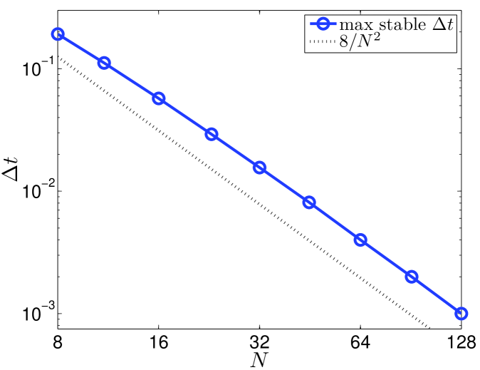
Figure 2: Scaling of maximum stable $\Delta t$ with $N$ for model PDE.

IV.2 Simulations of the BSSN system

This subsection documents results for simulations of the unit-mass-parameter ($M=1$) Schwarzschild solution (82) expressed in terms of ingoing Kerr-Schild coordinates. Since the solution is stationary, temporal integration of the semi-discrete scheme has been carried out with the forward Euler method which the dissipation in our method allows. The $r$-coordinate domain $[0.4,3.4]$ has been split into 3 equally spaced subdomains, and we have set $\eta=10$, $\lambda=0.1$, and $C=2$ [cf. Eq. (49)]. For all simulations $\Delta t$ has been chosen for stability. With the chosen $\lambda$, the inner physical boundary $r_{\mathrm{min}}=0.4$ is an excision surface. At each timestep we have applied an (order $2s=20$) exponential filter on the top two-thirds of the modal coefficient set for all fields except for $g_{rr}$ and $g_{\theta\theta}$. For stability, we have empirically observed that $g_{rr}$ and $g_{\theta\theta}$ must not be filtered. A detailed understanding of this is still lacking.

Issues related to physical boundary conditions are similar to the one encountered in Sec. IV.1 for the model problem. Similar to before, we have retained Eqs. (46,50) as the choice of numerical flux even at the endpoints. Therefore, at an endpoint the specification of the boundary condition amounts to the choice $W^{+}$ of external state. We have typically chosen the inner boundary of the radial domain as an excision boundary, and in this case $W^{+}=W^{-}$ is enforced at the inner physical boundary. At the outer physical boundary, for $W^{+}$ we have again considered two choices: (i) $W_{\mathrm{exact}}$ and (ii) $W_{\mathrm{upwind}}$. To enforce choice (ii) the inverse transformation (17) must be used with incoming characteristic fields fixed to their exact values, similar to (68). We have tried various versions of choice (ii), and in all cases the resulting simulations have been unstable. We therefore present results corresponding to choice (i). Although the choice of an analytical external state $W_{\mathrm{exact}}$ at the outer boundary is stable for our problem, such a boundary condition is unlikely to generalize to more complicated scenarios involving dynamical fields. Indeed, the issue of outer boundary conditions for the BSSN system is an active area of research, with a proper treatment requiring fixation of incoming radiation, control of the constraints, and specification of gauge (see Ref. NunezSarbach2009 for a recent analysis).

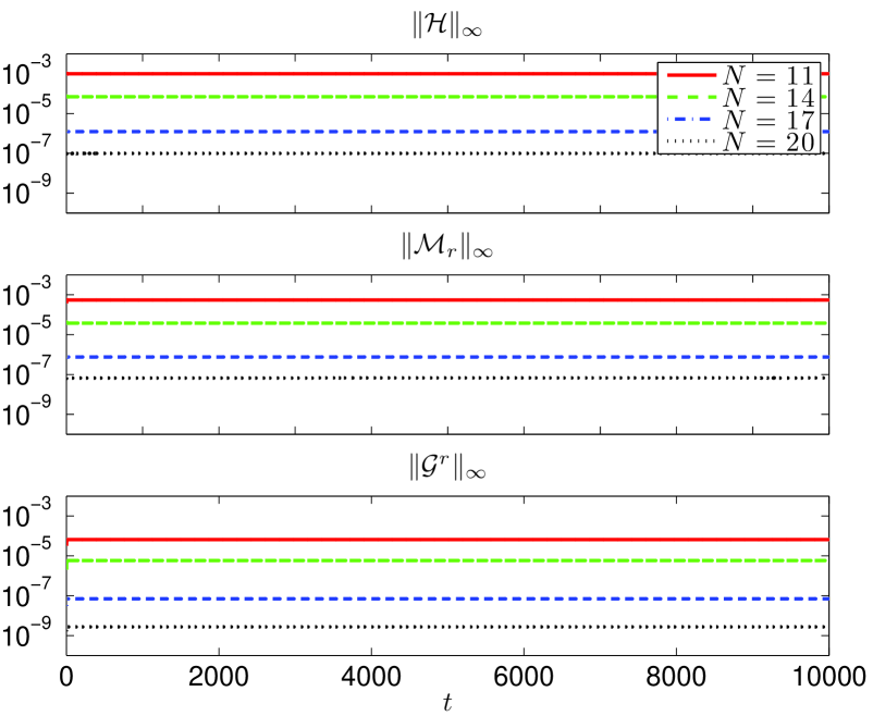
Figure 3: Spectral convergence of constraint violations for $M=1$ Kerr-Schild initial data. Respectively, for $N=11,14,17,19$, a timestep of $\Delta t\simeq 0.0041,0.0026,0.0018,0.0013$ has been chosen for stability and accuracy.

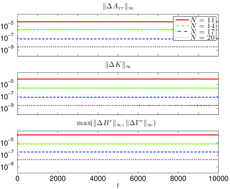
Figure 4: Spectral convergence of solution for $M=1$ Kerr-Schild initial data. Timestep choices are described in the caption for Fig. 3. In the title headings, for example, $\Delta A_{rr}\equiv(A_{rr})_{\mathrm{numer}}-(A_{rr})_{\mathrm{exact}}$.

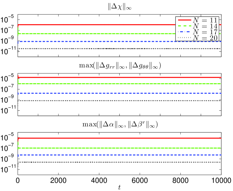
Figure 5: Spectral convergence of solution violations for $M=1$ Kerr-Schild initial data. See the caption of Fig. 4 for details.

For BSSN simulations, our main diagnostic is to monitor the Hamiltonian, momentum, and conformal connection constraints. Figure 3 depicts long-time histories of constraint violations, whereas Figs. 4 and 5 depict long-time error histories for the individual BSSN field components. From the middle plot in Fig. 5, we infer that, up to the indicated numerical error, the factor $g/\sin^{4}\theta=g_{rr}(g_{\theta\theta})^{2}$ remains at its initial fixed profile $r^{4}$ throughout the evolution. These figures indicate that the proposed scheme is stable for long times, and exhibits spectral converge with increased polynomial order $N$. Similar results are recovered from $M=0$ Minkowski initial data. The stability documented in these plots does not appear to rely on inordinate parameter tuning. For example, with the fixed parameters described above, we obtain similar plots if we individually vary (i) $r_{\mathrm{min}}$ over $\{0.325,0.35,0.4,0.475\}$ (values still corresponding to an excision surface for the given choice of $\lambda$), (ii) $\eta$ over $\{1,3,7,10\}$, (iii) $s$ over $\{8,9,10\}$. With the polynomial order $N$ ranging over $\{23,26,29,31\}$, both stability and qualitatively similar exponential convergence is achieved with a single subdomain. Likewise, adoption of a larger coordinate domain with more subdomains does not significantly impact our results. However, for much larger $r_{\mathrm{max}}$ stability requires a smaller time step or a time stepper better suited for wave problems (e.g. Runge Kutta 4). Finally, we have considered the addition of random noise to all field components at the initial time. Precisely, with the system component $\chi$ as an example, we have set

$$\boldsymbol{\chi}(0)\mapsto\boldsymbol{\chi}(0)+\delta\boldsymbol{\chi}(0),$$ (69)

where each component (nodal value) of $\delta\boldsymbol{\chi}(0)$ is $10^{-5}$ times a random variable drawn from a standard normal distribution. Such perturbed initial data also gives rise to stable evolutions.

V Conclusion

We have introduced a discontinuous Galerkin method for solving the spherically reduced BSSN system with second-order spatial operators. Our scheme shares similarities with other discontinuous Galerkin methods that use local auxiliary variables to handle high-order spatial derivatives Bassi ; CockburnShu ; ShuSchro ; ShuKvd ; Arnold_dG ; Brezzi_FluxChoice ; HEST , and which have typically been applied to either elliptic, parabolic, or mixed type problems. The key ingredient of a stable dG scheme is an appropriate choice of numerical flux, and our particular choice has been motivated by the analysis presented in Appendix C. When used to evolve the Schwarzschild solution in Kerr-Schild coordinates, our numerical implementation of the BSSN system (4) is robustly stable and converges to the analytic solution exponentially with increased polynomial order. By approximating the spatially second-order form of the BSSN system, we have not introduced extra fields which are evolved. Evolved auxiliary fields result in new constraints which may spoil stability. Our main goal has been stable evolution of the spherically reduced BSSN system as a first step towards understanding how a discontinuous Galerkin method might be applied to the full BSSN system. Towards that goal, we now discuss treatment of singularities and generalization of the described dG method to higher space dimension.

To deal with the fixed Schwarzschild singularity, we have used excision which is easy in the context of the spherically reduced BSSN system. However, excision for the binary black hole problem in full general relativity requires attention to the technical challenge of horizon tracking. State-of-the-art BSSN codes avoid such complication, relying instead on the moving-puncture technique. While the moving-puncture technique does involve mild central singularities, it may still prove amenable to spectral methods. Indeed, spectral methods for non-smooth problems is well-developed in both theory and for complex applications. Since the moving-puncture technique can be performed in spherical symmetry BrownSphSymBSSN , a first-step toward a spectral moving-puncture code would be to implement a moving puncture with the nodal dG method described here. Such an implementation may adopt Legendre-Gauss-Radau nodes on the innermost subdomain, thereby ensuring that the physical singularity does not lie on a nodal point (in much the same way finite difference codes use a staggered grid). Beyond traditional excision and moving punctures, one might construct smooth initial data via the turducken approach to singularities. However, in combination with 1+$\log$ slicing and the Gamma-driver shift condition, turduckened initial data will evolve towards a “trumpet” geometry Brown_Turducken1 ; Brown_Turducken2 .

Discontinuous Galerkin methods for hyperbolic problems in two and three space dimensions are well-developed. A generalization of the method described here to three-dimensions and the full BSSN system would likely rely on an unstructured mesh. Appropriate local polynomial expansions for the subelements are well-understood, as are choices for the numerical fluxes which would now live on two-dimensional faces rather than single points. Whether or not it would ultimately prove successful, generalization of our dG method to a higher dimension would rely on an established conceptual framework. Further computational advances of relevance to a generalization of our dG method to the full BSSN system (possibly including matter) may include mesh $hp$-adaptivity, local timestepping, shock capturing and slope limiting techniques HEST . Moreover, recent work KlocHestWar indicates that enhanced performance would be expected were our scheme implemented on graphics processor units.

VI Acknowledgments

We thank Nick Taylor for discussions about treating second-order operators with spectral methods, Benjamin Stamm for helping polish up a few parts of Appendix C, Khosro Shahbazi for discussions on LDG and IP methods. We also acknowledge helpful conversations with David Brown and Manuel Tiglio about the BSSN system and previous work on its numerical implementation. We gratefully acknowledge funding through grants DMS 0554377 and DARPA/AFOSR FA9550-05-1-0108 to Brown University and NSF grant PHY 0855678 to the University of New Mexico.

Appendix A Hyperbolicity of the first-order system.

This appendix analyzes the matrix $\mathcal{A}(u)$ appearing in (10) in order to construct the characteristic fields (14). In matrix form the sector (8) of the principal part of (10) reads as follows:

$$\partial_{t}\left[\begin{array}[]{c}B^{r}\\ \\ A_{rr}\\ \\ K\\ \\ \Gamma^{r}\\ \\ Q_{\chi}\\ \\ Q_{g_{rr}}\\ \\ Q_{g_{\theta\theta}}\\ \\ Q_{\alpha}\\ \\ Q_{\beta^{r}}\\ \end{array}\right]=\left[\begin{array}[]{ccccccccc}\beta^{r}&0&-\frac{4\lambda\alpha}{3g_{rr}}&0&0&\frac{\lambda\beta^{r}}{6(g_{rr})^{2}}&\frac{\lambda\beta^{r}}{3g_{\theta\theta}g_{rr}}&0&\frac{4\lambda}{3g_{rr}}\\ &&&&&&&&\\ 0&\beta^{r}&0&\frac{2}{3}g_{rr}\alpha\chi&\frac{1}{3}\alpha&-\frac{\alpha\chi}{3g_{rr}}&\frac{\alpha\chi}{3g_{\theta\theta}}&-\frac{2}{3}\chi&0\\ &&&&&&&&\\ 0&0&\beta^{r}&0&0&0&0&-\frac{\chi}{g_{rr}}&0\\ &&&&&&&&\\ 0&0&-\frac{4\alpha}{3g_{rr}}&\beta^{r}&0&\frac{\beta^{r}}{6(g_{rr})^{2}}&\frac{\beta^{r}}{3g_{\theta\theta}g_{rr}}&0&\frac{4}{3g_{rr}}\\ &&&&&&&&\\ 0&0&\frac{2}{3}\alpha\chi&0&\beta^{r}&-\frac{\beta^{r}\chi}{3g_{rr}}&-\frac{2\beta^{r}\chi}{3g_{\theta\theta}}&0&-\frac{2}{3}\chi\\ &&&&&&&&\\ 0&-2\alpha&0&0&0&\frac{2}{3}\beta^{r}&-\frac{2g_{rr}\beta^{r}}{3g_{\theta\theta}}&0&\frac{4}{3}g_{rr}\\ &&&&&&&&\\ 0&\frac{g_{\theta\theta}\alpha}{g_{rr}}&0&0&0&-\frac{g_{\theta\theta}\beta^{r}}{3g_{rr}}&\frac{1}{3}\beta^{r}&0&-\frac{2}{3}g_{\theta\theta}\\ &&&&&&&&\\ 0&0&-2\alpha&0&0&0&0&\beta^{r}&0\\ &&&&&&&&\\ \frac{3}{4}&0&0&0&0&0&0&0&\beta^{r}\end{array}\right]\left[\begin{array}[]{c}B^{r}\\ \\ A_{rr}\\ \\ K\\ \\ \Gamma^{r}\\ \\ Q_{\chi}\\ \\ Q_{g_{rr}}\\ \\ Q_{g_{\theta\theta}}\\ \\ Q_{\alpha}\\ \\ Q_{\beta^{r}}\end{array}\right]^{{}_{\mbox{\LARGE${}^{\prime}$}}},$$ (70)

which defines the matrix $\tilde{A}(u)$ appearing in (9), and so also the matrix $\mathcal{A}(u)$ in (10). Note that in the last equation the matrix within the square brackets is $-\tilde{A}(u)$. For certain configurations of $u$ and $\lambda$, the system (10) is strongly hyperbolic KreissLorenz , that is $\mathcal{A}(u)$ has a complete set of eigenvectors and real eigenvalues. Indeed, five eigenpairs of $\mathcal{A}(u)$ are trivially recovered upon inspection of $\mathcal{A}(u)$’s leading $5\times 5$ diagonal block. These correspond to eigenvalue 0 and the left eigenspace $\{\xi_{j}=e_{j}^{T}:1\leq j\leq 5\}$, where $e_{j}$ are the canonical basis vectors. Since each component of $u$ arises as $e_{j}^{T}W$, each is also a characteristic field.

The remaining nine eigenpairs are determined by $\tilde{A}(u)$. The eigenvalues of $\tilde{A}(u)$ are

$$\mu_{1}=0,\quad\mu_{2,3}=-\beta^{r},\quad\mu_{4}^{\pm}=-\beta^{r}\pm\sqrt{\frac{2\alpha\chi}{g_{rr}}},\quad\mu_{5}^{\pm}=-\beta^{r}\pm\alpha\sqrt{\frac{\chi}{g_{rr}}},\quad\mu_{6}^{\pm}=-\beta^{r}\pm\sqrt{\frac{\lambda}{g_{rr}}},$$ (71)

and the corresponding left eigenvectors are

$$x_{1} =(0,0,0,0,0,g_{\theta\theta},2g_{rr},0,0)$$ (72a)

$$x_{2} =\left(0,0,0,g_{rr},\frac{2}{\chi},-\frac{1}{2g_{rr}},-\frac{1}{g_{\theta\theta}},0,0\right)$$ (72b)

$$x_{3} =\left(\frac{g_{rr}}{\lambda},0,0,0,\frac{2}{\chi},-\frac{1}{2g_{rr}},-\frac{1}{g_{\theta\theta}},0,0\right)$$ (72c)

$$x_{4}^{\pm} =\left(0,0,\pm\sqrt{\frac{2\alpha g_{rr}}{\chi}},0,0,0,0,1,0\right)$$ (72d)

$$x_{5}^{\pm} =\left(0,\mp\frac{3}{\sqrt{g_{rr}\chi}},\pm 2\sqrt{\frac{g_{rr}}{\chi}},2g_{rr},\frac{1}{\chi},-\frac{1}{g_{rr}},\frac{1}{g_{\theta\theta}},0,0\right)$$ (72e)

$$x_{6}^{\pm} =\left(-\frac{3}{4}\frac{g_{rr}}{\lambda},0,\pm\frac{\alpha\sqrt{\lambda g_{rr}}}{(2\alpha\chi-\lambda)},0,0,-\frac{\beta^{r}}{8(\beta^{r}g_{rr}\mp\sqrt{\lambda g_{rr}})},\right.$$

$$\hskip 14.22636pt\left.-\frac{\beta^{r}g_{rr}}{4g_{\theta\theta}(\beta^{r}g_{rr}\mp\sqrt{\lambda g_{rr}})},\frac{\alpha\chi}{(2\alpha\chi-\lambda)},\pm\sqrt{\frac{g_{rr}}{\lambda}}\right),$$ (72f)

where for example $x_{5}^{\pm}\tilde{A}(u)=\mu_{5}^{\pm}x_{5}^{\pm}$. Assuming that $g_{rr}$, $g_{\theta\theta}$, $\chi$, and $\alpha$ are everywhere strictly positive, the eigenvalues are real and the eigenvectors are linearly independent provided that (15) holds. These eigenvectors are easily extended to eigenvectors of $\mathcal{A}(u)$, e. g. as $x_{6}^{\pm}\rightarrow(0_{1\times 5},x_{6}^{\pm})$. Then, for example, the characteristic field

$$X_{6}^{\pm}\equiv(0_{1\times 5},x_{6}^{\pm})W=x_{6}^{\pm}W_{v:Q},$$ (73)

and similarly $X_{j}^{\pm}=x^{\pm}_{j}W_{v:Q}$ for $j=4,5$ and $X_{k}=x_{k}W_{v:Q}$ for $k=1,2,3$. The characteristic speeds for these fields are $\mu_{k}$ and $\mu^{\pm}_{j}$. With this convention the speeds listed in Table 1 correspond to the $X_{k}$ and $X_{j}^{\pm}$ in (14).

Appendix B Schwarzschild solution in conformal Kerr-Schild coordinates.

In Kerr-Schild coordinates, here the system directly related to incoming Eddington-Finkelstein null coordinates, the line element for the Schwarzschild solution reads

$$ds^{2}=-\alpha^{2}dt^{2}+(1+2M/R)(dR+\beta^{R}dt)^{2}+R^{2}d\theta^{2}+R^{2}\sin^{2}\theta d\phi^{2},$$ (74)

where $R$ is the area radius, $\alpha=(1+2M/R)^{-1/2}$ is the lapse, and $\beta^{R}=2M/(R+2M)$ is the shift vector. The physical spatial metric $\bar{g}_{ab}$ is the spatial part of this line element.

To define the corresponding solution to the BSSN system, we use equation $g_{ab}=\chi\bar{g}_{ab}$ to define the following relationship between line elements:

$$dr^{2}+r^{2}(d\theta^{2}+\sin^{2}\theta d\phi^{2})=\chi[(1+2M/R)dR^{2}+R^{2}d\theta^{2}+R^{2}\sin^{2}\theta d\phi^{2}],$$ (75)

so that

$$\chi\left(1+\frac{2M}{R}\right)\left(\frac{dR}{dr}\right)^{2}=1,\qquad\chi R^{2}=r^{2}.$$ (76)

Then we have

$$\left(1+\frac{2M}{R}\right)^{1/2}\frac{dR}{R}=\frac{dr}{r},$$ (77)

with integration yielding

$$r=\frac{R}{4}\left(1+\sqrt{1+\frac{2M}{R}}\right)^{2}e^{2-2\sqrt{1+2M/R}},$$ (78)

where the constant of integration has been chosen so that the $R,r\rightarrow\infty$ limits are consistent. The second relation in (76) shows that

$$\chi=\frac{1}{16}\left(1+\sqrt{1+\frac{2M}{R}}\right)^{4}e^{4-4\sqrt{1+2M/R}},\qquad\chi^{-4}=\frac{2e^{\sqrt{1+2M/R}-1}}{1+\sqrt{1+2M/R}}.$$ (79)

The extrinsic curvature tensor is specified by the expression for $K$ given in (82h), the identity $K=K^{R}_{R}+2K^{\theta}_{\theta}$, and

$$K^{\theta}_{\theta}=\left(1+\frac{2M}{R}\right)^{-1/2}\frac{2M}{R^{2}}.$$ (80)

Since $K^{R}_{R}=K^{r}_{r}$, we compute that

$$K^{r}_{r}=K-2K^{\theta}_{\theta}=-\left(1+\frac{2M}{R}\right)^{-1/2}\left(\frac{R+M}{R+2M}\right)\frac{2M}{R^{2}}.$$ (81)

Next, since $K_{rr}=\bar{g}_{rr}K^{r}_{r}=\chi^{-1}K^{r}_{r}$, we have $K^{r}_{r}=A_{rr}+{\textstyle\frac{1}{3}}g_{rr}K$. This implies $A_{rr}=K^{r}_{r}-{\textstyle\frac{1}{3}}K$, from which we get (82g). In all we have

$$\alpha =\left(1+\frac{2M}{R}\right)^{-1/2}$$ (82a)

$$\beta^{r} =\beta^{R}\frac{dr}{dR}=\chi^{1/2}\left(1+\frac{2M}{R}\right)^{-1/2}\frac{2M}{R}$$ (82b)

$$g_{rr} =1$$ (82c)

$$g_{\theta\theta} =r^{2}=\chi R^{2}$$ (82d)

$$\chi =\frac{1}{16}\left(1+\sqrt{1+\frac{2M}{R}}\right)^{4}e^{4-4\sqrt{1+2M/R}}$$ (82e)

$$B^{r} =0$$ (82f)

$$A_{rr} =-\left(1+\frac{2M}{R}\right)^{-1/2}\frac{4M}{3R^{2}}\left(\frac{2R+3M}{R+2M}\right)$$ (82g)

$$K =\left(1+\frac{2M}{R}\right)^{-3/2}\left(1+\frac{3M}{R}\right)\frac{2M}{R^{2}}$$ (82h)

$$\Gamma^{r} =-\frac{2}{r}=-\frac{2}{\chi^{1/2}R}.$$ (82i)

To differentiate these expressions with respect to $r$, we use the identity

$$\frac{dR}{dr}=\chi^{-1/2}\left(1+\frac{2M}{R}\right)^{-1/2}$$ (83)

along with the chain rule.

Appendix C Stability of the model system

The following stability analysis for the model system (61) has been inspired by ShuSchro ; ShuKvd . After dropping all nonlinear source terms, the system (61) becomes

$$\partial_{t}u =u^{\prime}+av$$ (84a)

$$\partial_{t}v =u^{\prime\prime}+v^{\prime}.$$ (84b)

This section analyzes the stability of (84), considering both the continuum system itself as well as its semi-discrete dG approximation. The latter analysis offers some insight into the empirically observed stability of our dG scheme for the spherically reduced BSSN equations.

C.1 Analysis for a single interval

Throughout we work with the $L_{2}$ inner product and norm,

$$(f,g)_{\mathsf{D}}=\int_{\mathsf{D}}fg,\qquad\|f\|_{\mathsf{D}}=\sqrt{(f,f)_{\mathsf{D}}},$$ (85)

where $\mathsf{D}$ is the spatial coordinate interval (here $\mathsf{D}$ may represent a subdomain $\mathsf{D}^{k}$ or the whole domain $\Omega$), and we have suppressed all integration measures. For the continuum model we will establish the following estimate:

$$\|u^{\prime}(T,\cdot)\|^{2}_{\mathsf{D}}+a\|v(T,\cdot)\|^{2}_{\mathsf{D}}\leq C(T)\left(\|u^{\prime}(0,\cdot)\|^{2}_{\mathsf{D}}+a\|v(0,\cdot)\|^{2}_{\mathsf{D}}\right),$$ (86)

where the time-dependent constant $C(T)$ is determined solely by the choice of boundary conditions. To show (86), we first change variables with $\hat{v}=\sqrt{a}v$, thereby rewriting (84) in the following symmetric form:

$$\partial_{t}u =u^{\prime}+\sqrt{a}\hat{v}$$ (87a)

$$\partial_{t}\hat{v} =\sqrt{a}u^{\prime\prime}+\hat{v}^{\prime}.$$ (87b)

Equations (87a,b) then imply

$$\frac{1}{2}\partial_{t}\int_{\mathsf{D}}(u^{\prime})^{2} =\int_{\mathsf{D}}u^{\prime}(u^{\prime\prime}+\sqrt{a}\hat{v}^{\prime})=\int_{\mathsf{D}}\sqrt{a}u^{\prime}\hat{v}^{\prime}+\frac{1}{2}\int_{\partial\mathsf{D}}(u^{\prime})^{2}$$ (88a)

$$\frac{1}{2}\partial_{t}\int_{\mathsf{D}}(\hat{v})^{2} =\int_{\mathsf{D}}\hat{v}(\sqrt{a}u^{\prime\prime}+\hat{v}^{\prime})=-\int_{\mathsf{D}}\sqrt{a}u^{\prime}\hat{v}^{\prime}+\frac{1}{2}\int_{\partial\mathsf{D}}(\hat{v}{}^{2}+2\sqrt{a}u^{\prime}\hat{v}).$$ (88b)

Here $\hat{v}\hat{v}^{\prime}$ and $u^{\prime}u^{\prime\prime}$ have been expressed as exact derivatives and then integrated to boundary terms, the second equation employs an extra integration by parts, and with only one space dimension $\int_{\partial\mathsf{D}}$ denotes a difference of endpoint evaluations. Addition of Eqs. (88a,b) gives

$$\frac{1}{2}\partial_{t}\int_{\mathsf{D}}\big{[}\hat{v}{}^{2}+(u^{\prime})^{2}\big{]}=\frac{1}{2}\int_{\partial\mathsf{D}}\big{[}\hat{v}{}^{2}+(u^{\prime})^{2}+2\sqrt{a}u^{\prime}\hat{v}\big{]}.$$ (89)

Substitutions with the identities

$$\big{[}\hat{v}{}^{2}+(u^{\prime})^{2}\big{]}=\frac{1}{2}\big{[}(\hat{v}+u^{\prime})^{2}+(\hat{v}-u^{\prime})^{2}\big{]},\qquad 2u^{\prime}\hat{v}=\frac{1}{2}\big{[}(\hat{v}+u^{\prime})^{2}-(\hat{v}-u^{\prime})^{2}\big{]}$$ (90)

and replacements to recover the original variable $v=\hat{v}/\sqrt{a}$ yield

$$\frac{1}{2}\partial_{t}\int_{\mathsf{D}}\big{[}av^{2}+(u^{\prime})^{2}\big{]}=\frac{1+\sqrt{a}}{4}\int_{\partial\mathsf{D}}(\sqrt{a}v+u^{\prime})^{2}+\frac{1-\sqrt{a}}{4}\int_{\partial\mathsf{D}}(\sqrt{a}v-u^{\prime})^{2}.$$ (91)

From (91) we deduce that the time-dependent constant $C(T)$ in (86) must satisfy

$$\left|1+\frac{\int_{0}^{T}\left[\frac{1+\sqrt{a}}{2}\int_{\partial\mathsf{D}}(\sqrt{a}v+u^{\prime})^{2}+\frac{1-\sqrt{a}}{2}\int_{\partial\mathsf{D}}(\sqrt{a}v-u^{\prime})^{2}\right]dt}{\|u^{\prime}(0,\cdot)\|^{2}+a\|v(0,\cdot)\|^{2}}\right|\leq C(T).$$ (92)

For periodic boundary conditions, we may choose $C(T)=1$. Moreover, if $a\geq 1$ and $u^{\prime}=-\sqrt{a}v$ is specified at $\partial\mathsf{D}^{+}$, then $\|u^{\prime}(t,\cdot)\|^{2}+a\|v(t,\cdot)\|^{2}$ decays.

Still working on a single interval (subdomain), we now consider the semi-discrete scheme for (87), i. e. (65) with all nonlinear source terms dropped, and with $v$ replaced by $\hat{v}/\sqrt{a}$. Derivation of a formula analogous to (91) is our first step toward establishing $L_{2}$ stability of the semi-discrete scheme. While (65) features vectors, for example $\boldsymbol{u}(t)$, taking values at the Legendre-Gauss-Lobatto nodal points, here we work with the numerical solution as a polynomial, for example $u_{h}(t,x)$. These two representations are related by the Lagrange interpolating polynomials for the nodal set, here taken to span both the space of test functions and the space of basis functions. Our scheme is

$$\int_{\mathsf{D}^{k}}\psi\partial_{t}u_{h} =\int_{\mathsf{D}^{k}}\psi(Q_{h}+\sqrt{a}\hat{v}_{h})$$ (93a)

$$\int_{\mathsf{D}^{k}}\xi\partial_{t}\hat{v}_{h} =-\int_{\mathsf{D}^{k}}\xi^{\prime}(\sqrt{a}Q_{h}+\hat{v}_{h})+\int_{\partial\mathsf{D}^{k}}\xi(\sqrt{a}Q^{*}+\hat{v}{}^{*})$$ (93b)

$$\int_{\mathsf{D}^{k}}\varphi Q_{h} =\int_{\mathsf{D}^{k}}\varphi u_{h}^{\prime}+\int_{\partial\mathsf{D}^{k}}\varphi\left(u^{*}-u_{h}\right),$$ (93c)

where $\psi$, $\xi$, and $\varphi$ are polynomial test functions. These test functions are arbitrary, except that they must be degree-$N$ polynomials. In (93) the variables $u_{h}$, $\hat{v}_{h}$ and $Q_{h}$ should also carry a superscript $k$, but we have suppressed this. Derivation of a formula analogous to (91) is complicated by the fact that $Q_{h}$ is not evolved. Nevertheless, at a given instant $t$ we can assemble $Q_{h}$ from (93c).

Mimicking the calculation (88b) from the continuum case, we first use (93b) with $\xi=\hat{v}_{h}$ to write

$$\begin{split}\frac{1}{2}\partial_{t}\int_{\mathsf{D}^{k}}\hat{v}_{h}^{2}&=-\int_{\mathsf{D}^{k}}(\sqrt{a}Q_{h}+\hat{v}_{h})\hat{v}_{h}^{\prime}+\int_{\partial\mathsf{D}^{k}}(\sqrt{a}Q^{*}+\hat{v}{}^{*})\hat{v}_{h}\\ &=-\int_{\mathsf{D}^{k}}\sqrt{a}Q_{h}\hat{v}_{h}^{\prime}+\frac{1}{2}\int_{\partial\mathsf{D}^{k}}\big{[}2(\sqrt{a}Q^{*}+\hat{v}{}^{*})\hat{v}_{h}-\hat{v}_{h}^{2}\big{]}.\end{split}$$ (94)

The right-hand side of (88a) is analogous to

$$\frac{1}{2}\partial_{t}\int_{\mathsf{D}^{k}}Q_{h}^{2}=\int_{\mathsf{D}^{k}}Q_{h}\partial_{t}Q_{h}.$$ (95)

However, since $Q_{h}$ is not evolved, the term $\partial_{t}Q_{h}$ must be given a suitable interpretation. On the right hand side of (93c) only $u_{h}$, $u_{h}^{\prime}$, and $u^{*}$ necessarily depend on time, since the test function $\varphi$ need not be time-dependent. Furthermore, $u^{*}$ is explicitly given as a linear combination of $u_{h}$, as seen in Eq. (104c) below. Choosing $\varphi=\ell_{j}$, taking the time derivative of (93c), and appealing to the commutivity of mixed partial derivatives, we therefore arrive at

$$\int_{\mathsf{D}^{k}}\ell_{j}\partial_{t}Q_{h}=\int_{\mathsf{D}^{k}}\ell_{j}(\partial_{t}u_{h})^{\prime}+\int_{\partial\mathsf{D}^{k}}\ell_{j}\big{(}(\partial_{t}u)^{*}-\partial_{t}u_{h}\big{)},$$ (96)

where $(\partial_{t}u)^{*}$ depends on $\partial_{t}u_{h}$ in precisely the same way that $u^{*}$ depends on $u_{h}$. We have written $\ell_{j}$ rather than $\varphi$ in the last equation to emphasize that the result also holds for any linear combination of $\ell_{j}$ (for example $\varphi$), and even for time-dependent combinations. Since $Q_{h}$ is itself such a combination, we obtain

$$\begin{split}\frac{1}{2}\partial_{t}\int_{\mathsf{D}^{k}}Q_{h}^{2}&=\int_{\mathsf{D}^{k}}Q_{h}(\partial_{t}u_{h})^{\prime}+\int_{\partial\mathsf{D}^{k}}\big{(}(\partial_{t}u)^{*}-\partial_{t}u_{h}\big{)}Q_{h}\\ &=\int_{\mathsf{D}^{k}}Q_{h}(Q_{h}^{\prime}+\sqrt{a}\hat{v}_{h}^{\prime})+\int_{\partial\mathsf{D}^{k}}\big{(}(\partial_{t}u)^{*}-\partial_{t}u_{h}\big{)}Q_{h}\\ &=\int_{\mathsf{D}^{k}}\sqrt{a}Q_{h}\hat{v}_{h}^{\prime}+\frac{1}{2}\int_{\partial\mathsf{D}^{k}}\big{[}2((\partial_{t}u)^{*}-\partial_{t}u_{h})Q_{h}+Q_{h}^{2}\big{]}.\end{split}$$ (97)

Addition of (94) and (97) gives

$$\frac{1}{2}\partial_{t}\int_{\mathsf{D}^{k}}(Q_{h}^{2}+\hat{v}_{h}^{2})=\frac{1}{2}\int_{\partial\mathsf{D}^{k}}\big{[}Q_{h}^{2}-\hat{v}_{h}^{2}+2(\sqrt{a}Q^{*}+\hat{v}{}^{*})\hat{v}_{h}+2((\partial_{t}u)^{*}-\partial_{t}u_{h})Q_{h}\big{]},$$ (98)

the aforementioned analog of (91). This formula holds on a single subdomain $\mathsf{D}^{k}$, and we now combine multiple copies of it, one for each value of $k$.

C.2 Analysis for multiple intervals

To facilitate combination of (98) over all $k$, we change notation. At every subdomain interface $\mathsf{I}^{k+1/2}\equiv\partial\mathsf{D}^{k}\cap\partial\mathsf{D}^{k+1}$, let the superscripts $L$ and $R$ denote field values respectively taken from the left and right. Then the fields evaluated at $\mathsf{I}^{k+1/2}$ which belong to $\mathsf{D}^{k}$ will be $u_{k+1/2}^{L}$, $\hat{v}_{k+1/2}^{L}$, and $Q_{k+1/2}^{L}$, while those belonging to $\mathsf{D}^{k+1}$ will be $u_{k+1/2}^{R}$, $\hat{v}_{k+1/2}^{R}$, and $Q_{k+1/2}^{R}$. However, at $\mathsf{I}^{k-1/2}$ the values taken from $\mathsf{D}^{k}$ are $u_{k-1/2}^{R}$, $\hat{v}_{k-1/2}^{R}$, and $Q_{k-1/2}^{R}$. Note that we have also replaced the subscript $h$, denoting a numerical solution, with $k\pm 1/2$, denoting the location of the endpoint value of the numerical solution. With this notation, we define

$$\Delta^{L}_{\alpha}=\frac{1}{2}\left[(Q^{L}_{\alpha})^{2}-(\hat{v}^{L}_{\alpha})^{2}\right]+\left(\sqrt{a}Q_{\alpha}^{*}+\hat{v}_{\alpha}^{*}\right)\hat{v}^{L}_{\alpha}+\left[(\partial_{t}u_{\alpha})^{*}-\partial_{t}u_{\alpha}^{L}\right]Q^{L}_{\alpha},$$ (99)

and similarly for $\Delta^{R}_{\alpha}$. The same numerical fluxes appear in both $\Delta^{L}_{\alpha}$ and $\Delta^{R}_{\alpha}$ (i.e. each numerical flux takes the same value on either side of an interface), whence fluxes like $Q^{*}_{\alpha}$ do not carry an $L$ or $R$ superscript. In terms of these definitions (98) becomes

$$\frac{1}{2}\partial_{t}\int_{\mathsf{D}^{k}}(Q_{h}^{2}+\hat{v}_{h}^{2})=\Delta^{L}_{k+1/2}-\Delta^{R}_{k-1/2}.$$ (100)

Summation over all $\mathsf{D}^{k}$ yields

$$\frac{1}{2}\partial_{t}\sum_{k=1}^{k_{\mathrm{max}}}\int_{\mathsf{D}^{k}}(Q_{h}^{2}+\hat{v}_{h}^{2}) =\sum_{k=1}^{k_{\mathrm{max}}-1}\big{(}\Delta^{L}_{k+1/2}-\Delta^{R}_{k+1/2}\big{)}+\Delta^{L}_{k_{\mathrm{max}}+1/2}-\Delta^{R}_{1/2}$$

$$=\sum_{k=1}^{k_{\mathrm{max}}-1}\big{(}\Delta^{L}_{h}-\Delta^{R}_{h}\big{)}\big{|}_{\mathsf{I}^{k+1/2}}+\Delta^{L}_{k_{\mathrm{max}}+1/2}-\Delta^{R}_{1/2}.$$ (101)

We have reverted to $h$-notation denoting the numerical solution, since the $L,R$ superscripts indicate unambiguously the relevant domain used for evaluation at $\mathsf{I}^{k+1/2}$.

We again seek an estimate of the form

$$\sum_{k=1}^{k_{\mathrm{max}}}\big{(}\|Q_{h}(T,\cdot)\|^{2}_{\mathsf{D}^{k}}+a\|v_{h}(T,\cdot)\|^{2}_{\mathsf{D}^{k}}\big{)}\leq C(T)\sum_{k=1}^{k_{\mathrm{max}}}\big{(}\|Q_{h}(0,\cdot)\|_{\mathsf{D}^{k}}^{2}+a\|v_{h}(0,\cdot)\|_{\mathsf{D}^{k}}^{2}\big{)},$$ (102)

that is essentially the same as the one (86) considered in the continuum case. Assume that the chosen boundary conditions ensure $\Delta^{L}_{k_{\mathrm{max}}+1/2}-\Delta^{R}_{1/2}$ is bounded by a time-dependent constant which does not depend on the numerical parameters $N$ and $h$ (subdomain width). Establishment of stability then amounts to showing that the remaining sum over interface terms in (C.2) is non-positive; whence this remaining sum is consistent with $C(T)\leq 1$, although the boundary conditions may give rise to a different bound. In fact, we will choose the numerical fluxes such that each individual interface term is non-positive. At interface $\mathsf{I}^{k+1/2}$ and in $L,R$ notation, the jump and average of $\hat{v}_{h}$, for example, are

$$\frac{1}{2}\left(\hat{v}^{+}+\hat{v}^{-}\right)\equiv\{\!\{\hat{v}_{h}\}\!\} =\frac{1}{2}\left(\hat{v}^{L}_{k+1/2}+\hat{v}^{R}_{k+1/2}\right)$$ (103a)

$$\mathbf{n}^{-}\hat{v}^{-}+\mathbf{n}^{+}\hat{v}^{+}\equiv\big{[}\!\big{[}\hat{v}_{h}\big{]}\!\big{]} =\hat{v}^{L}_{k+1/2}-\hat{v}^{R}_{k+1/2}.$$ (103b)

Consider numerical fluxes of the form

$$Q^{*} =\{\!\{Q_{h}\}\!\}-\frac{\tau_{Q}}{2}\big{[}\!\big{[}Q_{h}\big{]}\!\big{]}$$ (104a)

$$\hat{v}{}^{*} =\{\!\{\hat{v}_{h}\}\!\}-\frac{\tau_{v}}{2}\big{[}\!\big{[}\hat{v}_{h}\big{]}\!\big{]}$$ (104b)

$$u^{*} =\{\!\{u_{h}\}\!\}-\frac{\tau_{u}}{2}\big{[}\!\big{[}u_{h}\big{]}\!\big{]}$$ (104c)

$$(\partial_{t}u)^{*} =\{\!\{\partial_{t}u_{h}\}\!\}-\frac{\tau_{u}}{2}\big{[}\!\big{[}\partial_{t}u_{h}\big{]}\!\big{]},$$ (104d)

where (104c) induces (104d) and where the penalty parameters $\tau_{u}$, $\tau_{v}$, and $\tau_{Q}$ are real numbers. The fluxes defined in (66) correspond to $\tau_{u}=1$, $\tau_{v}=1+\sqrt{a}$, and $\tau_{Q}=0$. In terms of these quantities the $k$th interface contribution in (C.2) is

$$\begin{split}(\Delta^{L}_{h}&-\Delta^{R}_{h})\big{|}_{\mathsf{I}^{k+1/2}}=\frac{1}{2}\left(\big{[}\!\big{[}Q_{h}^{2}\big{]}\!\big{]}-\big{[}\!\big{[}\hat{v}_{h}^{2}\big{]}\!\big{]}\right)+\{\!\{\hat{v}_{h}\}\!\}\big{[}\!\big{[}\hat{v}_{h}\big{]}\!\big{]}-\frac{\tau_{v}}{2}\big{[}\!\big{[}\hat{v}_{h}\big{]}\!\big{]}^{2}\\ &+\sqrt{a}\{\!\{Q_{h}\}\!\}\big{[}\!\big{[}\hat{v}_{h}\big{]}\!\big{]}-\frac{\sqrt{a}\tau_{Q}}{2}\big{[}\!\big{[}Q_{h}\big{]}\!\big{]}\big{[}\!\big{[}\hat{v}_{h}\big{]}\!\big{]}-\{\!\{Q_{h}\}\!\}\big{[}\!\big{[}\partial_{t}u_{h}\big{]}\!\big{]}-\frac{\tau_{u}}{2}\big{[}\!\big{[}\partial_{t}u_{h}\big{]}\!\big{]}\big{[}\!\big{[}Q_{h}\big{]}\!\big{]},\end{split}$$ (105)

where we have suppressed the $k$ dependence of the right-hand side. Now consider the term $\big{[}\!\big{[}\partial_{t}u_{h}\big{]}\!\big{]}$. Because $\partial_{t}u_{h}$ and $Q_{h}+\sqrt{a}\hat{v}_{h}$ are both polynomials of degree $N$, Eq. (93a) implies the vector equation $\partial_{t}\boldsymbol{u}=\boldsymbol{Q}+\sqrt{a}\hat{\boldsymbol{v}}$, that is pointwise equivalence on the nodal points of $\mathsf{D}^{k}$, which in turn implies $\big{[}\!\big{[}\partial_{t}u_{h}\big{]}\!\big{]}=\big{[}\!\big{[}Q_{h}+\sqrt{a}\hat{v}_{h}\big{]}\!\big{]}$. Upon substituting this identity into the last equation, we arrive at an expression which features only $\hat{v}_{h}$ and $Q_{h}$,

$$\begin{split}(\Delta^{L}_{h}&-\Delta^{R}_{h})\big{|}_{\mathsf{I}^{k+1/2}}=\frac{1}{2}\left(\big{[}\!\big{[}Q_{h}^{2}\big{]}\!\big{]}-\big{[}\!\big{[}\hat{v}_{h}^{2}\big{]}\!\big{]}\right)+\{\!\{\hat{v}_{h}\}\!\}\big{[}\!\big{[}\hat{v}_{h}\big{]}\!\big{]}-\frac{\tau_{v}}{2}\big{[}\!\big{[}\hat{v}_{h}\big{]}\!\big{]}^{2}\\ &+\sqrt{a}\{\!\{Q_{h}\}\!\}\big{[}\!\big{[}\hat{v}_{h}\big{]}\!\big{]}-\frac{\sqrt{a}\tau_{Q}}{2}\big{[}\!\big{[}Q_{h}\big{]}\!\big{]}\big{[}\!\big{[}\hat{v}_{h}\big{]}\!\big{]}-\{\!\{Q_{h}\}\!\}\big{[}\!\big{[}Q_{h}+\sqrt{a}\hat{v}_{h}\big{]}\!\big{]}-\frac{\tau_{u}}{2}\big{[}\!\big{[}Q_{h}+\sqrt{a}\hat{v}_{h}\big{]}\!\big{]}\big{[}\!\big{[}Q_{h}\big{]}\!\big{]}.\end{split}$$ (106)

The identities $\{\!\{\hat{v}_{h}\}\!\}\big{[}\!\big{[}\hat{v}_{h}\big{]}\!\big{]}=\frac{1}{2}\big{[}\!\big{[}\hat{v}_{h}^{2}\big{]}\!\big{]}$ and $\big{[}\!\big{[}Q_{h}+\sqrt{a}\hat{v}_{h}\big{]}\!\big{]}=\big{[}\!\big{[}Q_{h}\big{]}\!\big{]}+\sqrt{a}\big{[}\!\big{[}\hat{v}_{h}\big{]}\!\big{]}$ then simplify (106) to

$$(\Delta^{L}_{h}-\Delta^{R}_{h})\big{|}_{\mathsf{I}^{k+1/2}}=-\frac{\tau_{v}}{2}\big{[}\!\big{[}\hat{v}_{h}\big{]}\!\big{]}^{2}-\frac{\sqrt{a}(\tau_{u}+\tau_{Q})}{2}\big{[}\!\big{[}Q_{h}\big{]}\!\big{]}\big{[}\!\big{[}\hat{v}_{h}\big{]}\!\big{]}-\frac{\tau_{u}}{2}\big{[}\!\big{[}Q_{h}\big{]}\!\big{]}^{2}.$$ (107)

The role of a penalty parameter is now clear. Positive values of $\tau_{v}$ penalize jumps in $\hat{v}_{h}$ through a negative contribution to the energy. Likewise, positive values of $\tau_{u}$ penalize jumps in $Q_{h}$ through a negative contribution to the energy. However, because the sign of $\big{[}\!\big{[}Q_{h}\big{]}\!\big{]}\big{[}\!\big{[}\hat{v}_{h}\big{]}\!\big{]}$ can be positive or negative, only the choice $\tau_{Q}=-\tau_{u}$ yields an expression for $(\Delta^{L}_{h}-\Delta^{R}_{h})|_{\mathsf{I}^{k+1/2}}$ which is manifestly negative for $\tau_{u}\geq 0$ and $\tau_{v}\geq 0$. A simple estimate based on Young’s inequality with $\varepsilon$ (that is, $2\alpha\beta\leq\varepsilon^{-1}\alpha^{2}+\varepsilon\beta^{2}$, where $\alpha,\beta\geq 0$ and $\varepsilon>0$) shows that for $\tau_{Q}=0$ the choice $\tau_{v}\geq a\tau_{u}/4$ also yields stability.

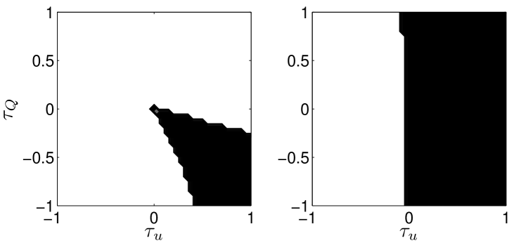
Figure 6: Stable evolutions for the model system. For fixed $\tau_{v}=10^{-6}$ and $\tau_{v}=1+\sqrt{2}$ respectively, the left and right plots depict stable choices (determined empirically) of $\tau_{u}$ and $\tau_{Q}$ for the linear model system (84). The stable regions are colored black, but the jagged edges result from the discretization of the $(\tau_{u},\tau_{Q})$-plane.

Figure 6 depicts certain choices of stable penalty parameters for the linear model system evolved to $t_{\mathrm{final}}=1000$ (with $a=2$, $N=10$, and $\Delta t\simeq 0.0553$), as determined empirically with simulations similar to those described in Sec. IV.1. The left plot corresponds to a small $\tau_{v}=10^{-6}$, for which the choice $\tau_{u}=1$, $\tau_{Q}=0$ is not stable, as expected from the theoretical analysis. However, the right plot corresponds to $\tau_{v}=1+\sqrt{a}$, for which $\tau_{u}=1$, $\tau_{Q}=0$ is stable. Motivated by the numerical flux choices (46,50) used for the BSSN system (4), we have (as mentioned above) set $\tau_{u}=1$, $\tau_{v}=1+\sqrt{a}$, and $\tau_{Q}=0$ in simulations of the nonlinear model (61). For the nonlinear model system (61), the theoretically motivated choice $\tau_{Q}=-\tau_{u}$ also yields numerically stable evolutions when $\tau_{u}\geq 0$ and $\tau_{v}\geq 0$.

For the nonlinear systems (4) and (61), we do not attempt a formal stability proof. Nevertheless, the results of this appendix have served as a guide for our choices of penalty parameters. For the BSSN system (4), $u$, $v$, and $Q$ are block indices [cf. Eq. (6)]. Similar to the model problem, we have penalized $Q$ with $\tau_{u}=1$, with $\tau_{v}$ chosen large enough to heuristically overcome the cross-terms of indefinite size that arise from $\tau_{Q}=0$ (we interpret equations like $\tau_{u}=1$ componentwise). An analogous choice “$\tau_{Q}=-\tau_{u}$” for the BSSN system might be possible, but would be considerably more complicated. Indeed, such a choice likely entails a matrix of penalty parameters, but we do not give the details here.

References

- (1) F. Pretorius, Evolution of Binary Black-Hole Spacetimes, Phys. Rev. Lett. 95, 121101 (2005) (4 pages).
- (2) F. Pretorius, Simulation of binary black hole spacetimes with a harmonic evolution scheme, Class. Quantum Grav. 23, S529-S552 (2006).
- (3) M. Campanelli, C. O. Lousto, P. Marronetti, and Y. Zlochower, Accurate Evolutions of Orbiting Black-Hole Binaries without Excision, Phys. Rev. Lett. 96, 111101 (2006) (4 pages).
- (4) J. G. Baker, J. Centrella, D.-I. Choi, M. Koppitz, and J. van Meter, Gravitational-Wave Extraction from an Inspiraling Configuration of Merging Black Holes, Phys. Rev. Lett. 96, 111102 (2006) (4 pages).
- (5) M. Campanelli, C. O. Lousto, and Y. Zlochower, Last orbit of binary black holes, Phys. Rev. D 73, 061501(R) (2006) (5 pages).
- (6) F. Herrmann, I. Hinder, D. Shoemaker, and P. Laguna, Unequal mass binary black hole plunges and gravitational recoil, Class. Quantum Grav. 24, S33-S42 (2007).
- (7) P. Diener, F. Herrmann, D. Pollney, E. Schnetter, E. Seidel, R. Takahashi, J. Thornburg, and J. Ventrella, Accurate Evolution of Orbiting Binary Black Holes, Phys. Rev. Lett. 96, 121101 (2006) (4 pages).
- (8) M. A. Scheel, H. P. Pfeiffer, L. Lindblom, L E. Kidder, O. Rinne, and S. A. Teukolsky, Solving Einstein’s Equations With Dual Coordinate Frames, Phys. Rev. D 74 104006 (2006).
- (9) U. Sperhake, Binary black-hole evolutions of excision and puncture data, Phys. Rev. D 76, 104015 (2007) (20 pages).
- (10) B. Brügmann, J. A. González, M. Hannam, S. Husa, U. Sperhake, and W. Tichy, Calibration of moving puncture simulations, Phys. Rev. D 77, 024027 (2008) (25 pages).
- (11) P. Marronetti, W. Tichy, B. Brügmann, J. González, M. Hannam, S. Husa and U. Sperhake, Binary black holes on a budget: simulations using workstations, Class. Quantum Grav. 24, S43-S58 (2007).
- (12) Z. B. Etienne, J. A. Faber, Y. T. Liu, S. L. Shapiro, and T. W. Baumgarte, Filling the holes: Evolving excised binary black hole initial data with puncture techniques, Phys. Rev. D 76, 101503(R) (2007) (5 pages).
- (13) B. Szilágyi, D. Pollney, L. Rezzolla, J. Thornburg, and J. Winicour, An explicit harmonic code for black-hole evolution using excision, Class. Quantum Grav. 24, S275-S293 (2007).
- (14) L. Boyle, M. Kesden, and S. Nissanke, Binary-Black-Hole Merger: Symmetry and the Spin Expansion, Phys. Rev. Lett. 100, 151101 (2008) (4 pages).
- (15) M. A. Scheel, M. Boyle, T. Chu, L. E. Kidder, K. D. Matthews, and H. P. Pfeiffer, High-accuracy waveforms for binary black hole inspiral, merger, and ringdown, Phys. Rev. D 79, 024003 (2009) (14 pages).
- (16) M. Hannam, Status of black-hole-binary simulations for gravitational-wave detection, Class. Quantum Grav. 26, 114001 (2009) (21 pages).
- (17) I. Hinder, The current status of binary black hole simulations in numerical relativity, Class. Quantum Grav. 27, 114004 (2010) (19 pages).
- (18) B. P. Abbott et al., LIGO: The Laser Interferometer Gravitational-Wave Observatory, Rep. Prog. Phys. 72, 076901 (2009) (25 pages).
- (19) F. Acernese et al., The status of VIRGO, Class. Quantum Grav. 23, S63-S69 (2006).
- (20) F. Acernese et al., Virgo status, Class. Quantum Grav. 25, 184001 (2008) (9 pages).
- (21) R. Arnowitt, S. Deser, and C. W. Misner, The Dynamics of General Relativity, in Gravitation: an introduction to current research, edited by L. Witten (Wiley, New York, 1962), Chapter 7, 227-265. Also available as gr-qc/0405109.
- (22) J. W. York, Jr., Kinematics and Dynamics of General Relativity, in Sources of Gravitational Radiation, edited by L. L. Smarr (Cambridge University Press, Cambridge, 1979).
- (23) L. E. Kidder, M. A. Scheel and S. A. Teukolsky, Extending the lifetime of 3D black hole computations with a new hyperbolic system of evolution equations, Phys. Rev. D 64, 064017 (2001) (13 pages).
- (24) G. Calabrese, J. Pullin, O. Sarbach and M. Tiglio, Convergence and stability in numerical relativity, Phys. Rev. D 66, 041501(R) (2002) (4 pages).
- (25) S. Frittelli and O. Reula, On the Newtonian Limit of General Relativity, Commun. Math. Phys. 166, 221-235 (1994).
- (26) M. Shibata and T. Nakamura, Evolution of three-dimensional gravitational waves: Harmonic slicing case, Phys. Rev. D 52, 5428-5444 (1995).
- (27) Y. Choquet-Bruhat and J. W. York, Geometrical well posed systems for the Einstein equations, C. R. Acad. Sci. Paris, t. 321, Série I, 1089-1095 (1995).
- (28) A. Abrahams, A. Anderson, Y. Choquet-Bruhat, and J. W. York, Jr., Einstein and Yang-Mills Theories in Hyperbolic Form without Gauge Fixing Phys. Rev. Lett. 75, 3377-3381 (1995).
- (29) C. Bona, J. Massó, E. Seidel, and J. Stela, New Formalism for Numerical Relativity, Phys. Rev. Lett. 75, 600-603 (1995).
- (30) M. H. P. M. van Putten and D. M. Eardley, Nonlinear wave equations for relativity, Phys. Rev. D 53, 3056-3063 (1996).
- (31) S. Frittelli and O. A. Reula, First-Order Symmetric Hyperbolic Einstein Equations with Arbitrary Fixed Gauge, Phys. Rev. Lett. 76, 4667-4670 (1996).
- (32) H. Friedrich, Hyperbolic reductions for Einstein’s equations, Class. Quantum Grav. 13, 1451-1469 (1996).
- (33) F. B. Estabrook, R. S. Robinson, H. D. Wahlquist, Hyperbolic equations for vacuum gravity using special orthonormal frames, Class. Quantum Grav. 14, 1237-1247 (1997).
- (34) M. S. Iriondo, E. O. Leguizamón, and O. A. Reula, Einstein’s Equations in Ashtekar’s Variables Constitute a Symmetric Hyperbolic System, Phys. Rev. Lett. 79, 4732-4735 (1997).
- (35) A. Anderson, Y. Choquet-Bruhat, and J. W. York, Einstein-Bianchi hyperbolic system for general relativity, Topol. Meth. Nonlinear Anal. 10, 353-373 (1997).
- (36) T. W. Baumgarte and S. L. Shapiro, Numerical integration of Einstein’s field equations, Phys. Rev. D 59 024007 (1998) (7 pages).
- (37) M. Á. G. Bonilla, Symmetric hyperbolic systems for Bianchi equations, Class. Quantum Grav. 15, 2001-2005 (1998).
- (38) G. Yoneda and H. Shinkai, Symmetric Hyperbolic System in the Ashtekar Formulation, Phys. Rev. Lett. 82, 263-266 (1999).
- (39) M. Alcubierre, B. Brügmann, M. Miller, and W.-M. Suen, Conformal hyperbolic formulation of the Einstein equations, Phys. Rev. D 60, 064017 (1999) (4 pages).
- (40) S. Frittelli and O. A. Reula, Well-posed forms of the 3+1 conformally-decomposed Einstein equations J. Math. Phys. 40, 5143-5156 (1999).
- (41) A. Anderson and J. W. York, Jr., Fixing Einstein’s Equations, Phys. Rev. Lett. 82, 4384-4387 (1999).
- (42) S. D. Hern, Numerical Relativity and Inhomogeneous Cosmologies, Ph.D. dissertation, University of Cambridge, 1999. Also available as gr-qc/0004036.
- (43) H. Friedrich and A. Rendall, The Cauchy problem for the Einstein equations, in Einstein’s Field Equations and their Physical Implications, edited by B. G. Schmidt, Springer Lecture Notes in Physics, vol. 540, pp. 127-223 (Springer-Verlag, Berlin, 2000).
- (44) G. Yoneda and H. Shinkai, Constructing Hyperbolic Systems in the Ashtekar Formulation of General Relativity, Int. J. Mod. Phys. D 9, 13-34 (2000).
- (45) H. Shinkai and G. Yoneda, Hyperbolic formulations and numerical relativity: experiments using Ashtekar’s connection variables, Class. Quantum Grav. 17, 4799-4822 (2000).
- (46) G. Yoneda and H. Shinkai, Hyperbolic formulations and numerical relativity: II. asymptotically constrained systems of Einstein equations, Class. Quantum Grav. 18, 441-462 (2001).
- (47) L. E. Kidder, M. A. Scheel, S. A. Teukolsky, Extending the lifetime of 3D black hole computations with a new hyperbolic system of evolution equations, Phys. Rev. D 64, 064017 (2001) (13 pages).
- (48) C. Gundlach, G. Calabrese, I. Hinder and J. M. Martín-García, Constraint damping in the Z4 formulation and harmonic gauge, Class. Quantum Grav. 22, 3767-3773 (2005).
- (49) F. Pretorius, Numerical relativity using a generalized harmonic decomposition, Class. Quantum Grav. 22, 425-451 (2005)
- (50) J. D. Brown, Conformal invariance and the conformal-traceless decomposition of the gravitational field, Phys. Rev. D 71, 104011 (2005) (12 pages).
- (51) L. Lindblom, M. A. Scheel, L. E. Kidder, R. Owen, and O. Rinne, A new generalized harmonic evolution system, Class. Quantum Grav. 23, S447-S462 (2006).
- (52) R. Owen, Constraint damping in first-order evolution systems for numerical relativity, Phys. Rev. D 76, 044019 (2007) (11 pages).
- (53) V. Fock, The Theory of Space Time and Gravitation (Pergamon Press, New York, 1959).
- (54) http://www.black-holes.org/SpEC.html
- (55) N. W. Taylor, L. E. Kidder, and S. A. Teukolsky, Spectral methods for the wave equation in second-order form, arXiv:1005.2922v1[gr-qc].
- (56) N. W. Taylor, personal communication.
- (57) W. Tichy, Black hole evolution with the BSSN system by pseudospectral methods, Phys. Rev. D 74, 084005 (2006) (10 pages).
- (58) W. Tichy, Long term black hole evolution with the BSSN system by pseudospectral methods, Phys. Rev. D 80, 104034 (2009) (10 pages).
- (59) A. H. Mroue, personal correspondence.
- (60) M. Hannam, S. Husa, D. Pollney, B. Brügmann, and N. Ó Murchadha, Geometry and Regularity of Moving Punctures, Phys. Rev. Lett. 99, 241102 (2007) (4 pages).
- (61) M. Hannam, S. Husa, B. Brügmann, J. A. González, U. Sperhake, and N. Ó Murchadha, Where do moving punctures go?, J. Phys.: Conf. Ser. 66, 012047 (2007) (9 pages).
- (62) J. D. Brown, BSSN in spherical symmetry, Class. Quantum Grav. 25, 205004 (2008) (23 pages).
- (63) T. W. Baumgarte and S. G. Naculich, Analytical representation of a black hole puncture solution, Phys. Rev. D 75, 067502 (2007) (4 pages).
- (64) M. Hannam, S. Husa, F. Ohme, B. Brügmann, and N. Ó Murchadha, Wormholes and trumpets: the Schwarzschild spacetime for the moving-puncture generation, Phys. Rev. D 78, 064020 (2008) (19 pages).
- (65) J. D. Brown, Probing the puncture for black hole simulations, Phys. Rev. D 80, 084042 (2009) (24 pages).
- (66) J. D. Brown, Puncture evolution of Schwarzschild black holes, Phys. Rev. D 77, 044018 (2008) (5 pages).
- (67) J. S. Hesthaven, S. Gottlieb, and D. Gottlieb, Spectral Methods for Time-Dependent Problems (Cambridge University Press, Cambridge UK, 2007).
- (68) J. S. Hesthaven and T. Warburton, Nodal Discontinuous Galerkin Methods: Algorithms, Analysis, and Applications (Springer, New York, 2008).
- (69) K. Shahbazi, An explicit expression for the penalty parameter of the interior penalty method, J. Comp. Phys. 205, issue 2, 401-407 (2005).
- (70) Y. Cheng and C.-W. Shu, A discontinuous Galerkin finite element method for time dependent partial differential equations with higher order derivatives, Math. Comp. 77, no. 262, 699-730 (2007).
- (71) M. J. Grote, A. Schneebeli, and D. Schötzau, Discontinuous Galerkin finite element method for the wave equation, SIAM J. Numer. Anal. 44, no. 6, 2408-2431 (2006).
- (72) M. J. Grote, A. Schneebeli, and D. Schötzau, Interior penalty discontinuous Galerkin method for Maxwell’s equations: Energy norm error estimates, J. Comp. Appl. Math. 204, issue 2, 375-386 (2007).
- (73) J. S. Hesthaven and T. Warburton, Nodal High-Order Methods on Unstructured Grids. I. Time-Domain Solution of Maxwell’s Equations, J. Comp. Phys. 181, issue 1, 186-221 (2002).
- (74) A. Schneebeli, Interior Penalty Discontinuous Galerkin Methods for Electromagnetic and Acoustic Wave Equations, Ph.D. dissertation, University of Basel, 2006. Also available as http://edoc.unibas.ch/diss/DissB_7760.
- (75) H. Friedrich and A. D. Rendall, The Cauchy Problem for the Einstein Equations, Lec. Notes Phys. 540, 127-224 (2000). Also available as arXiv:gr-qc/0002074v1.
- (76) C. Gundlach and J. M. Martin-Garcia, Symmetric hyperbolic form of systems of second-order evolution equations subject to constraints, Phys. Rev. D 70, 044031 (2004) (14 pages).
- (77) C. Gundlach, J. M. Martin-Garcia, Hyperbolicity of second-order in space systems of evolution equations, Class. Quantum Grav. 23, S387-S404 (2006).
- (78) H.-O. Kreiss and J. Lorenz, Initial-Boundary Value Problems and the Navier-Stokes Equations, SIAM Classics in Applied Mathematics (SIAM, Philadelphia, 2004).
- (79) B. Cockburn and C.-W. Shu, The local discontinuous Galerkin method for time-dependent convection-diffusion systems, SIAM J. Numer. Anal. 35, no. 6, 2440-2463 (1998).
- (80) Y. Xu, C.-W. Shu, Local discontinuous Galerkin methods for nonlinear Schrödinger equations, J. Comp. Phys. 205, issue 1, 72-97 (2005).
- (81) Y. Xu, C.-W. Shu, Local discontinuous Galerkin methods for the Kuramoto-Sivashinsky equations and the Ito-type coupled KdV equations, Comp. Methods Appl. Mech. Engin. 195, 3430-3447 (2006).
- (82) M. Alcubierre, B. Brügmann, P. Diener, M. Koppitz, D. Pollney, E. Seidel, and R. Takahashi, Gauge conditions for long-term numerical black hole evolutions without excision, Phys. Rev. D 67, 084023 (2003) (18 pages).
- (83) G. H. Golub and C. F. Van Loan, Matrix Computations, third edition (John Hopkins University Press, Baltimore and London, 1996).
- (84) F. Bassi and S. Rebay, A High-Order Accurate Discontinuous Finite Element Method for the Numerical Solution of the Compressible Navier-Stokes Equations, J. Comp. Phys. 131, issue 2, 267-279 (1997).
- (85) S. E. Field, J. S. Hesthaven, and S. R. Lau, Discontinuous Galerkin method for computing gravitational waveforms from extreme mass ratio binaries, Class. Quantum Grav. 26, 165010 (2009) (28 pages).
- (86) F. Brezzi, G. Manzini, D. Marini, P. Pietra, and A. Russo, Discontinuous finite elements for diffusion problems, in Atti Convegno in onore di F. Brioschi (Milan, 1997), 197-217. Istituto Lombardo, Accademia di Scienze e Lettere, Milan, Italy, 1999.
- (87) D. N. Arnold, F. Brezzi, B. Cockburn, and L D. Marini, Unified analysis of discontinuous Galerkin methods for elliptic problems, SIAM J. Numer. Anal. 39, no. 5, 1749–1779 (2002).
- (88) D. Núñez and O. Sarbach, Boundary conditions for the Baumgarte-Shapiro-Shibata-Nakamura formulation of Einstein’s field equations, Phys. Rev. D 81, 044011 (2010) (16 pages).
- (89) D. Brown, P. Diener, O. Sarbach, E. Schnetter, and M. Tiglio, Turduckening black holes: An analytical and computational study, Phys. Rev. D 79, 044023 (2009) (19 pages).
- (90) D. Brown, O. Sarbach, E. Schnetter, M. Tiglio, P. Diener, I. Hawke, and D. Pollney, Excision without excision, Phys. Rev. D 76, 081503(R) (2007) (5 pages).
- (91) A. Klöckner, T. Warburton, J. Bridge, and J. S. Hesthaven, Nodal discontinuous Galerkin methods on graphics processors, J. Comp. Phys. 228, issue 21, 7863-7882 (2009).