The Geometry of Oriented Cubes
Macquarie University Research Report No: 86-0082
Abstract
This reports on the fundamental objects revealed by Ross Street, which he called ‘orientals’. Street’s work was in part inspired by Robert’s attempts [8] to use -category ideas to construct nets of -algebras in Minkowski space for applications to relativistic quantum field theory: Roberts’ additional challenge was that “no amount of staring at the low dimensional cocycle conditions would reveal the pattern for higher dimensions”.
This report takes up this challenge, presents a natural inductive construction of explicit cubical cocyle conditions, and gives three ways in which the simplicial ones can be derived from these. A consequence of this work is that the Yang-Baxter equation, the ‘pentagon of pentagons’, and higher simplex equations, are in essence different manifestations of the same underlying abstract structure.
There has been recent interest in higher-categories, by computer scientists investigating concurrency theory, as well as by physicists, among others. The dual ‘string’ version of this paper, originally presented in [2], and which motivated much of the role of cubes in [10], makes clear the relationship with higher-dimensional simplex equations in physics.
Much work in this area has been done since these notes were written: no attempt has been made to update the original report. However, all diagrams have been redrawn by computer, replacing all original hand-drawn pictures.
We obtain a geometric interpretation of Street’s simplicial orientals, by describing an oriental structure on the -cube. This corresponds to describing nested sequences of embedded disks in the boundary of the -cube, obtained consecutively as ordered deformations keeping the boundaries fixed. Canonical forms for the order are obtained, leading to definitions of cocycle conditions for application to non-abelian cohomology in a category.
1 Introduction
Street [9] has defined an -category structure on the -simplex, leading to his notion of . This was motivated by an approach to non-abelian cohomology, arising from quantum field theory [8], but also seems to have intriguing connections with homotopy coherence, loop space desuspension and the cobar construction, as well as the realisation of homotopy types. Intimately related to Street’s structure on simplices is an analogous one on cubes, from which the simplicial results can be derived. This paper takes up Roberts’ challenge [8] that “no amount of staring at the low dimensional cocycle conditions would reveal the pattern for higher dimensions”. The result is surprisingly simple, natural and beautiful. We define and describe this finer structure of oriented cubes, from a geometric point of view. This makes obvious the relevance to homotopy theory.
This paper is self-contained, presupposing minimal familiarity with either category theory or homotopy theory. Categorical aspects and applications will be discussed in a subsequent paper.
Consider the following geometric reasoning: In obstruction theory applied to simplicial or cubical complexes, a standard problem is the continuous extension of data defined on the boundary of a cell (usually a simplex or cube). Although the boundary of such a cell is a geometrically decomposed sphere, the only structure used involves assigning alternating signs appropriately to the sub-cells of the decomposition. If we wish to keep the spherical structure in mind, we can imagine the boundary sphere of the cell decomposed as two hemispheres, with an extension over the cell of the data assigned to the hemispheres now viewed as a continuous deformation, keeping the boundary data fixed, between the assignments of data to each of the hemispheres. Since the boundary of each hemisphere is also a sphere, it is natural to seek splittings of spheres in every dimension.
Suppose we have some “data” defined over a sphere, and two possibly distinct extensions over a cell. By viewing two cells as upper and lower hemispheres, we may instead consider this as an extension, over a sphere of one dimension higher, of data assigned to the “equatorial” sphere. We can then think of the two extensions over the hemispheres as being “equivalent” in some sense if the data assigned to this higher sphere extends over a cell. But there may be another such extension, tantamount to an alternative equivalence, which enables us to bootstrap the procedure. At any stage, we see data on a sphere, split as two hemispheres, with data on the equatorial sphere, which in turn splits as two hemispheres, whose boundary sphere splits as two hemispheres, and so on.
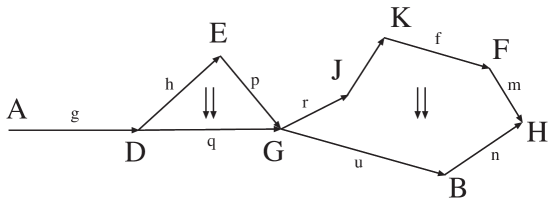
Consider now category theory, viewing arrows (or morphisms) as one dimensional cells whose boundary 0-spheres split as the union of a source and a target - which we view as 0-dimensional points. If we consider a 2-category (see [6] for example), we see that 2-cells have a 1-dimensional source and target, each of which is an ordinary arrow in a category, and both of which have the same 0-dimensional source and target. Thus we see the boundary of a 2-cell split into two hemispheres, and the boundary of each hemisphere similarly split. (Figure 1)
Street’s structure on simplices [9] allows an interpretation as a coherent version, across all dimensions, of a structure as described above. Our purpose is to exhibit such a structure on the -dimensional cube. This leads to the notion of a “-dimensional source” and “-dimensional target” of the -cube, for each , just as a 2-cell in a 2-category has sources in dimensions 0 and 1. Amusingly, the answer suggests a curious connection with -forms on . From a categorical viewpoint this decomposition leads to the notion of an -.
2 The structure of the -cube
Denote by the (ordered) set , and by . Let denote the interval in the real number axis, and the (geometric) -dimensional cube. We think of a point as the 0-dimensional cube or simplex.
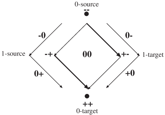
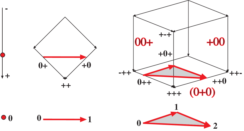
Dimension 1: In Figure 2 we have a single , with a notion of source (“0-source”) and target. We may think of this as an arrow assigned to the interval . As a convention, we choose “” to be considered the source and “” the target. Hence the dichotomy “source/target” arises from the disconnectedness of the 0-sphere . It is convenient for “” (respectively “”) to be considered synonymous with “” (respectively ). Moreover, we use “” to denote the whole interval:
Observe that has three sub-cubes, and . When we take the product with the unit interval we obtain , to which each sub-cube of contributes three sub-cubes. These can be thought of as a new copy, an old copy and a thickened copy. Proceeding inductively we see that has sub-cubes. More precisely, let .
Proposition 2.1: There is a 1:1 correspondence between (geometric) sub-cubes of and elements of .
Thus we may define the n-cube to be , and call an element of a - of . We will henceforth use the notation , or occasionally [], to denote the -cube, and no longer use .
Notation: Since each is ordered, an element of can be specified as a word of length in the symbols of .
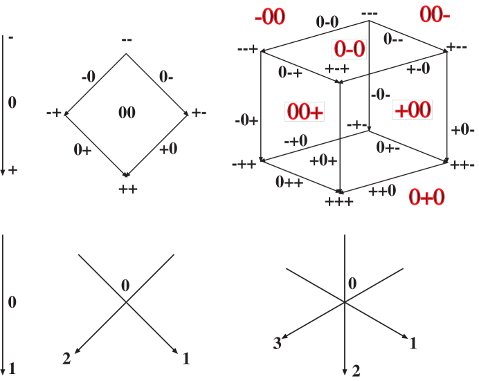
Example 2.2: In Figure 2 we draw the 1, 2, and 3 dimensional cubes, labeled according to the usual convention arising from the unit interval in .
Define maps by
These add to the right of a word the symbols and respectively, and can be thought of as the old, thickened and new copies of .
Definition 2.3: The of , denoted by , is the cardinality of .
This is the number of 0’s occurring in the word-form of , and induces a grading by setting .
There are three distinguished subcubes of , which in word form are , and . We shall respectively refer to the latter two as the 0-source and 0-target of , denoted by and . More generally we will define and for each . These are to be thought of as “-dimensional source” and “-dimensional target” of respectively. We shall suppress some symbols when the context is clear.
For each of dimension and , we can define a new element . Set ( if . If , listed in increasing order, define by performing on and otherwise, using the natural order: (. This gives a pairing
Note that this defines an associative operation as with matrix multiplication.
We may think of any such as a -cube placed in . More generally we can use to place any set of sub-cubes of the -cube into . Once we define and on , we can extend to by , and similarly for .
3 Motivational examples
We examine the lowest dimensional cubes to elucidate their structure:
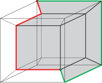
Dimension 2: The boundary of consists of four edges and four vertices. To each of the edges is assigned naturally, given our convention, an orientation. This canonically determines the source and target in dimension 0, as shown in Figure 3. Since the edge (respectively ) arises as the thickened 0-source (respectively 0-target) of , a natural criterion for choosing the one dimensional source and target for is determined. Hence we may assign a “double arrow” to , pointing from the 1-source to the 1-target. Note that geometrically the boundary circle (1-sphere) of is decomposed into two hemispheres, each having as boundary the 0-source and 0-target.
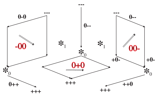
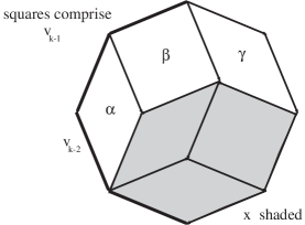
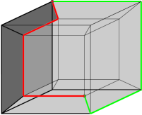
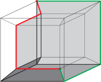
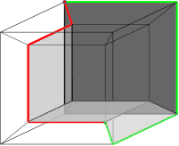
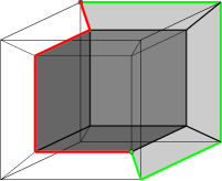
Dimension 3: In Figure 4, we thicken the various subcubes of to obtain the usual description of . Again the 0-dimensional sources and targets are determined, as are the 1-dimensional ones. Observe that the 1-source and 1-target are symmetrically defined, and that each consists of a copy of the 2-dimensional ones, suitably shifted by the third dimension, together with a thickened 0-dimensional source or target. Applying the same reasoning to the definition of 2-source and 2-target as we did for dimension 1, we see the 2-source and 2-target of as depicted in Figure 5. The boundary of is a
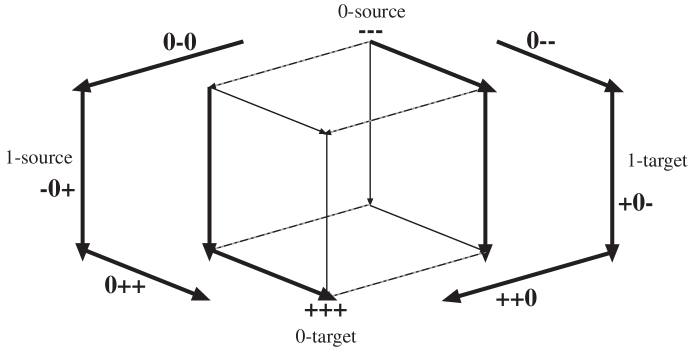
2-sphere splitting as two hemispheres, the 2-dimensional source (at the back) and target (at front) of , which in turn have boundary 1-sphere splitting as two hemispheres, the 1-dimensional source and target of , which in turn have boundary 0-sphere splitting as two hemispheres, the 0-dimensional source and target of .
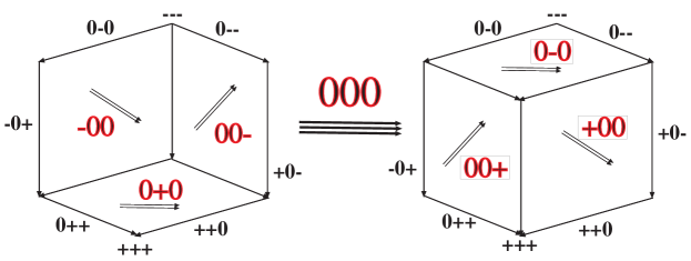
Remark: Although there is obvious appeal in the simplicity of the preceding description of the 2-source and 2-target of as the union of three s each, observe that the s concerned do not have the same 0-source and 0-target, nor the same 1-source and 1-target. Hence a little care is required to get the definitions correct. At this level, the answer both algebraically and geometrically is provided by the notions of 2-category theory and the middle-interchange law ([6, 9]). This is described in Figure 6. Each of the s comprising the 2-source of must be stretched out by an appropriate to the 0-source or 0-target of .
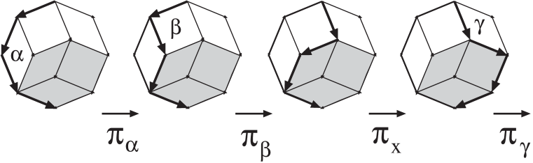
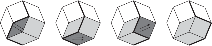
An interpretation of this goes as follows: each 1-dimensional path from the 0-source to the 0-target can be thought of as the trace of a deformation or homotopy of the 0-source to the 0-target, consecutively across the arrows forming the path. See Figure 7. In , there are only two possible paths, the 1-source and the 1-target, and itself can be thought of as providing a deformation from the 1-source to the 1-target. For , there are four possible paths for each of the 2-source and 2-target.
In the same way, each of the 2-source and 2-target can be thought of as deformations, in three stages each, of the 1-source to the 1-target. The source deformations must be carried out in the order shown in Figure 8. This is because we cannot deform a 1-path across a unless all of the 1-source of the in question is part of the 1-path. Each such deformation leaves unchanged the rest of the 1-path, and the number of segments in the path remains the same. Each component of the 2-source consists of a across which part of the 1-path is being deformed, and the remainder
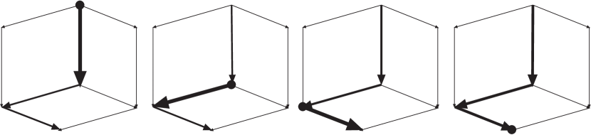
of the 1-path. From another viewpoint, the s string out the s, providing the path by which the 0-source of can be deformed to the 0-source of the relevant . This gives rise to the composition of 2-category theory.
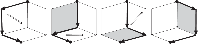
Note that in this case we are composing cubes stuck end-to-end, source-to-target, along the 0-dimensional (geometric) sources and targets. The s, on the other hand, are glued together along 1-dimensional source/target paths. This corresponds to in the language of 2-categories.The geometry is exactly that of 2-categorical pasting diagrams. (See for example [6].)
Thus not only are the constituent parts of the 2-source of derived from the structure of , but a natural order emerges for their 2-categorical order of composition. This order in turn derives entirely from our initial convention for source and target of . We also note that the 2-cubes of the source or target fit together in such a way that the deformations are possible, and compatibly with the structure defined on .
4 Source and target faces - Piles
We require to have sources and targets in all dimensions . These allow us to deform the ()-source, across either the -dimensional source or target, onto the (-1)-target. The (-1)-source is made up of s as well as lower dimensional cubes. The lower dimensional cubes stretch out each to the sources and targets of in all dimensions ().
In deforming the -source across to the (-target, such lower dimensional cubes play a role; we will not be able to push across a given unless all of lower dimensional sources have been reached. The order in which we proceed is determined inductively, necessitated by the need to expose all lower dimensional sources as required (compare Figure 8). The notion of “pile” enables us to describe the procedure to any desired degree of refinement. A pile is a list of all s we have reached at any stage of the deformation. Thus there are source and target piles, and intermediate piles. Each time we deform across a we alter the pile in all dimensions less than , since we deform from the source of that to its target in lower dimensions. In this way sub-cubes act as “operators” on piles. The order of deformation is then determined by groupings of sub-cubes as “blocks”. These blocks are characterised in that the initial and final piles on which they act respectively contain the -dimensional source and target faces of the in question. The -dimensional sources and targets of this are themselves blocks, acting on the piles corresponding to the still lower dimensional sources and targets.
Our immediate concern is to develop an appropriate formalism and notation to make these ideas concise for the -cube. We take an inductive approach starting with the raw material above.
For we saw that there are three s making up the 2-dimensional source. If we ignore the order in which these cubes are written, as well as their position in , we have a set of s we shall call the - of . More generally we will define the source and target - of , denoted and respectively. For given , we obtain two sequences of sets , and . The subscript indicates the dimension of elements of the set.
Definition 4.1: Let , and , for each . Inductively define a) For even:
b) For odd:
We have deliberately written these as (inductively) ordered, since the order reflects their sequence of operation on piles. A simple induction from the motivational examples proves
Theorem 4.2: (i) Identifying elements of either or along common boundaries produces a -dimensional disk . (ii)
Examples 4.3: In the following table we list the source and target faces for .
[n] [1] 0 0 0 0 0 0 0 0 [2] [3] [4]
Denote by the binomial coefficients arising in Pascal’s triangle.
Definition 4.4: An - is a sequence of () sets , such that (a) (b) each has cardinality (c) each has dimension .
Fix , and denote the collections of source and target faces by
Proposition 4.5: and are -piles.
Remark 4.6: Each sub--cube of the -cube is parallel to a subspace of . The subspaces arising in this fashion correspond to choices of elements of as subscripts for coordinate axes. Thus there are possible such subspaces, and for each, parallel copies in the boundary of . We shall call the collection of all such parallel copies a . Observe that the inductive definition of source and target faces canonically chooses a representative from each parallel set.
Definition 4.7: We will call any choice of a unique representative from each parallel set of -dimensional subcubes a -.
Hence Theorem 4.3 tells us that there are at least two distinct -sections whose topological union is a disc. Moreover, these unions are coherent across dimensions.
Note also that differential -forms in -space admit a basis analogous to a -section. This suggests some relationship to de Rham cohomology.
For each , , we define and as (-piles by using to embed elements of and into .
The definitions given above lead to the structure referred to in the introduction. We describe the relationship between the source- and target--piles, and how these relate to the cocycle conditions.
Proposition 4.8: For each , , where the antipodal map is the involution sending a word to , obtained from by interchanging each and . Hence and are interchanged by the antipodal map on [].
Remark 4.9: Since the parallel set to which a sub-cube belongs is determined by the position of 0’s in its word form, the antipodal map preserves parallel sets.
If now we have an -pile into which there exists an embedding for some , we obtain a new list by replacing by . Note that if , . We have a map , whose source and target are ()-piles. The top dimensional cube of (merely itself) remains in the pile, only its lower dimensional faces changing. (Here we abuse notation somewhat as may occur in many different ()-piles.)
Denote by the operation which applies the involution “” to every element of , . The operation will denote the identity. If now we begin with a pile and an embedding , it may be possible to find sequences
such that a sequence of piles is generated from , each obtained from the previous by applying consecutively the and . Observing that is parallel set preserving, it is not difficult to prove
Proposition 4.10: If is a pile for which each is a -section whose topological union, identifying along common boundaries, is a disk with boundary invariant under the antipodal map, the same is true for ) or ) whenever these are defined. Furthermore, the boundary of each such disc remains the same.
The - of [n], denoted , will be such a sequence containing , such that the composite of the sequence has source and target but with replacing . By applying the involution “” to the sequence written in reverse order we will find another such sequence, which we call the - of . This has source pile with replaced by . The sequence uses each element of , and has target .
Definition 4.11: The formal equality is called the (- .
5 Modifying piles - Blocks
Intuitively a pile describes a nested set of disks of descending dimension, geometrically embedded in the -cube. is the ()-source in some stage of (cubical) isotopy or deformation across the interior of , keeping the boundary fixed. The disc in practice is either the ()-source or target of . In turn each is the ()-source of after some deformation across , keeping the boundary fixed. Each disk decomposes as a set , the list of “currently encountered” -dimensional faces of as we deform across the cubes of . (See Figure 8.)
Suppose at some stage we have a pile such that for , and wish to apply for . This requires that the ()-, ()-,.., 0-faces of appear in the appropriate . In general this will not be the case. By looking at we can decide if there is any chance of applying . If has source faces appearing in , it should be possible to use the remaining -cubes in to change the lower ’s until the rest of the source faces of appear. We illustrate this schematically in Figure 9. The -source cubes of are those shaded among the cubes of .
The heavy path depicts , from which it is clear the (-source faces of do not all appear. Hence we apply consecutively , , then , and finally to obtain a pile with replaced by . If we now apply , having used all of the faces of in the sequence of applications, we can replace by and try to find the next cube higher up the list to apply. We illustrate in Figure 10.
Remark 5.1: There are two things to note here. The first is that to apply all of ’s lower dimensional source faces must appear in the pile. We may first have to apply the same process as above, at a lower dimension. Secondly we have the “moral” of the heuristic description: to apply , for , we must work in conjunction with the remaining s of . Hence occurs as part of a “block” of cubes, namely and the rest of the cubes in which are not in . This “block” is on the one hand derived from the pile, and on the other, composed of cubes which serve to modify the pile so that the process can continue. The conclusion is that every time we apply , , there is an associated “sweep” of the ()-source of across to the ()-target, at some stage sweeping across . All of these “sweeps” occur at different dimensions simultaneously.
We can try to find an order in which to proceed directly from the pile , in order to use all of the elements of to change each lower into the corresponding . This order will not be unique. However, knowing an order from the previous dimension will enable us to make inductively a natural choice.
Note that the effect of , , on ) can be decomposed : alters elements, an effect which can be obtained in stages corresponding to the effect of each ()-source-face of applied consecutively (and similarly target faces). Each of these can be further decomposed, all the way down to dimension . In Figure 11 we break up the effect of of the previous figure.
To present the procedure by which a canonical order of pile modifications is determined by the cocycle conditions, we seek an order for the application of elements of a “block”.
Definition 5.2: For odd, an - is a column of (, )-blocks. For even, an - is a row of (, )-blocks. An - is an element of .
Note 5.3: We do not require that the number of blocks occurring at any stage has any specific value, nor that they have equal size.
Example 5.4: Below we give examples of a -block for . Note that vertical and horizontal bars serve well to divide up the blocks. A block is “read” from left to right, top to bottom, and from smaller to larger sub-blocks. These give the -sources for the -, 2- ,3- and 4-cubes respectively:
|
|
|
|
||||||||||||||||||||||||||||||||||||||||||||||||||||||||||
Blocks can be written in a unique linear form, where when two -sub-blocks are separated by a bar, we write . We obtain, for each of the ‘sources’ just given in the previous table,
-
1.
-
2.
-
3.
-
4.
Remark 5.5: An equivalent definition of a -block on a set can be given. A -block is a pair where and , for some . Note that for an ordered set, we obtain something very much like a span.
Definition 5.6: By a -sub-block of a -block we will mean any sub-block characterized by elements between a pair , for , such that no occurs between them for . A full -sub-block will be a -sub-block maximal with respect to this condition.
For each word above, replace in the string by . Interpret each as “rewrite as for each ”, where is the word length.
For (c) we obtain the sequence of piles in the following Table 2. The 12 columns correspond to the geometric figures in Figure 12. Those on the left and right are those of and . The elements of each are shown in bold, and the hatched element is the appropriate for which is about to be applied. This illustrates the “nestings” of disks referred to earlier.
Proposition 5.7: The 0, 1-, 2-, 3-cocycle conditions are given by (1)–(4) above.
Table 2 - the 2-cocycle source of the 3-cube
We can tabulate part of the effect of the block (d) on by recording the changes at the 2-dimensional level. (We can always ignore the changes lower down in the pile to save space in description.) Since the highest dimension of occurring for any application of is 3, the set remains unaltered. The reader may wish to refer forward to the “octagon of octagons” depicted in Figure 7, comparing the lists of 2-cubes above with the left hand side configurations in the figure.
Table 3 – the source 3-cube action on source 2-cubes of the 4-cube
We denote by the set of -blocks of elements of . Note that there are natural inclusions , and an isomorphism . The can be used to define a structure analogous to the occurring in Street [9]. Note that there is a “forgetful” map which sends a -block to its underlying set of elements of . We can thus define the dimension of to be the maximum of the dimensions of its elements.
Definition 5.8: A distinguished -block is a -block for which each sub--block has all but one sub-(-1)-blocks of dimension , the other (-1)-block of dimension . We will denote by the subset of distinguished blocks. A 0-block is always considered distinguished.
Examples 5.9: All of the examples given above are distinguished. Our inductive definition of cocycles will demonstrate that all cocycles are distinguished. The notion makes precise how an element of a pile can only be applied in conjunction with those elements of a pile of the next lower dimension which do not occur as source faces of . Thus must be “stretched out” appropriately to the source and target of the whole pile.
Writing out the terms using the provides not only the order in which to modify the (-piles, but also tells us at which stage we must rewrite the pile from below the -dimensional level. Moreover, a separating two blocks and indicates that geometrically the respective collections of cubes are “glued together” along a -dimensional disk . itself is a collection of subcubes, and has a pile/block description as the the -target of and the -source of .
6 Sources and targets - inductive cocycles
We use the order defining the ()-source of to obtain the ()-source of . Since is obtained geometrically by thickening the )-cube, all of the cubes in the expression of the ()-source of will play a role in the form of either old, new or thickened copies, via the sources and targets they themselves have in lower dimensions. All -blocks subsequently considered will be distinguished, unless otherwise stated. Our intention is to describe how to complete the table for all , :
| [1] | 0 | 0 | 0 | |||||||||||||||||||||||||||||||||||||||||||||||||||||||||||||||||||||||||||||||||||
|---|---|---|---|---|---|---|---|---|---|---|---|---|---|---|---|---|---|---|---|---|---|---|---|---|---|---|---|---|---|---|---|---|---|---|---|---|---|---|---|---|---|---|---|---|---|---|---|---|---|---|---|---|---|---|---|---|---|---|---|---|---|---|---|---|---|---|---|---|---|---|---|---|---|---|---|---|---|---|---|---|---|---|---|---|---|---|
| [2] |
|
|||||||||||||||||||||||||||||||||||||||||||||||||||||||||||||||||||||||||||||||||||||
| [3] |
|
|
||||||||||||||||||||||||||||||||||||||||||||||||||||||||||||||||||||||||||||||||||||
| [4] |
|
|
|
Table 3 – for small
We shall only need to consider , . It is easy to list the sub--cubes of which occur, but the tricky part is to pin down and order those lower dimensional subcubes which stretch out the s to and for .
We shall inductively define functions
- (a)
-
For the -cube [], define = [] = . Hence these are 0-blocks (and -blocks by default.)
- (b)
-
For 0-blocks, define maps and by respectively. Extend the definition to an arbitrary -block by operating on each sub-0-block. (In practice symbolically this will partly involve adding .)
- (c)
-
Define = , and . This is the geometrically obvious choice. Extend the definition to , as described using . For an arbitrary -block, define and by restricting to the first 0-block.
- (d)
-
Define the 1-blocks and inductively by
These coincide with and respectively. Extend the definition of and to . For , set
This means that all of the columns are to be strung together, one on top of the next. For , we define the 1-source and 1-target by restricting to the first column. Geometrically think of the column as a string of subcubes joined together along their 0-sources and 0-targets. Taking the 1-source then strings together the s making up the 1-sources of the elements of the initial column. Note that for an arbitrary 1-block, 0-sources and 0-targets will not match, but those with which we are inductively concerned do continue to enjoy this property.
- (e)
-
Define : by
Hence and . Extend the domain of and to by application to each sub-1-block. Note that and “stretch out” the ends of a string of s arising from , which stretched between the 0-source and 0-target of , to the 0-source and 0-target of .
- (f)
-
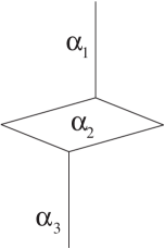
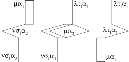
Figure 13: The source thickens - (g)
-
To define and on we use triple induction, first on , then , then . For = , = 0, we have already given the definition for “pure” cubes. Extension to is carried out as above.
All that is required is to avoid loops in our definitions. For we extend the domain to by consecutively defining [2], [2], and
This makes precise the way in which the 1-dimensional sources and targets of contribute to the 2-dimensional sources of .
We now wish to extend the domain to . It is here that the notion of distinguished k-block is crucial. In each 1-block, every sub-0-block except possibly one, , say, has dimension 1. These sub-blocks have trivial 2-dimensional sources, and serve to connect the 0-sources of the 1-block to the 0-source of , and similarly for the 0-targets of and . By induction, has sources and targets in lower dimensions. For ( we obtain a 2-block, each 1-block of which stretches between the 0-source and 0-target of . In order to define of the 1-block , we must stretch out each of the 1-blocks of ) by adding to each column a copy of the preceding s of at the top, and those succeeding at the bottom. We illustrate this in Figure 14.
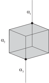
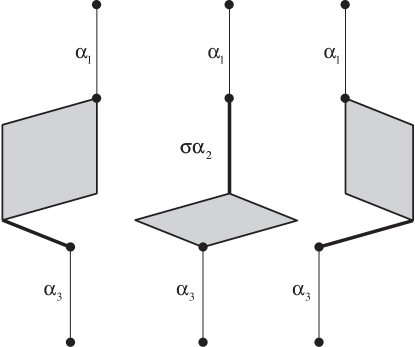
Figure 14: Stretching out lower dimensional sources and targets of distinguished blocks : . Left is the block with distinguished 3-cube; on the right, three 2-cubes are stretched out. Note that the resulting 2-block is again distinguished. The same procedure will be repeated in higher dimensions. Thus we extend the domain of to by setting
Here we have written the superscript “” to indicate multiple copies will be taken, since is a 2-block. This is 2-category pasting again.
To define on 2-blocks, apply it as defined above consecutively to each sub-1-block, juxtaposing the 2-blocks so obtained from left to right in the original order of the 1-blocks. For , define to be of the first sub-2-block.
- (h)
-
We now presume all maps defined for subscripts , on all . To define :
For even, define
For odd we set
This allows us to define for all blocks after we set for . To extend the definition to higher blocks, we use the intuition we have of the underlying geometry. A -block corresponds to a possibly higher dimensional cube , together with a number of others of dimension , each “filled out” by lower dimensional cubes. Then and should correspond to the -cubes already present, together with or of , with everything still appropriately stretched out by lower dimensional cubes. We merely break up the action of on the pile sets , , as the composition of the action of its -dimensional faces.
Specifically, to define , where is a -block,
() If , define to be applied to the first -block of .
() For , define to be the juxtaposition of applied to the consecutive ()-blocks of . Hence we need only be specific for .
() If has dimension , we set . Otherwise there is a 0-block contained in a unique sub-(-1)-block of dimension . Since is a -block, we stretch it out by the same sub-blocks which stretch out inside . Now is contained in a 1-block, with 0-blocks above and below. We add these 0-blocks above and below every 1-block of .
() Similarly, occurs in a unique 2-block, with 1-blocks occurring before and after the 1-block in which occurs. We thus add each of these 1-blocks appropriately before and after every 1-block of .
() Proceeding in this way, up to the highest dimensional block, we fill out to obtain the -block we define to be .
The procedure/definition merely tells us that if an element has been stretched out by lower dimensional cubes, we use these to stretch out the components of .
where again is the distinguished sub-block, and repetitions are required for the other blocks. We proceed similarly for and for the case even.
- (i)
-
Now define, for odd, and by
For k even, set
- (j)
-
Now define for k odd
For k even,
Having defined and for , it is possible to define a structure on the infinite dimensional cube, characterised as
Notions of well-formedness of subsets of can be given as in [9], using the cocycle conditions, and it is straightforward to prove
Proposition 6.1: There is an -category structure defined on .
Proposition 6.2: (i) If is a full -sub-block of , then = for , and similarly for targets. (ii) If is an occurence of consecutive -blocks of , then . Moreover, topologically the union of sub-cubes of is a disk of dimension . (iii) The piles generated by applications of elements of the cocycle blocks are nested embeddings of -disks with geometric boundary .
7 Low dimensional examples
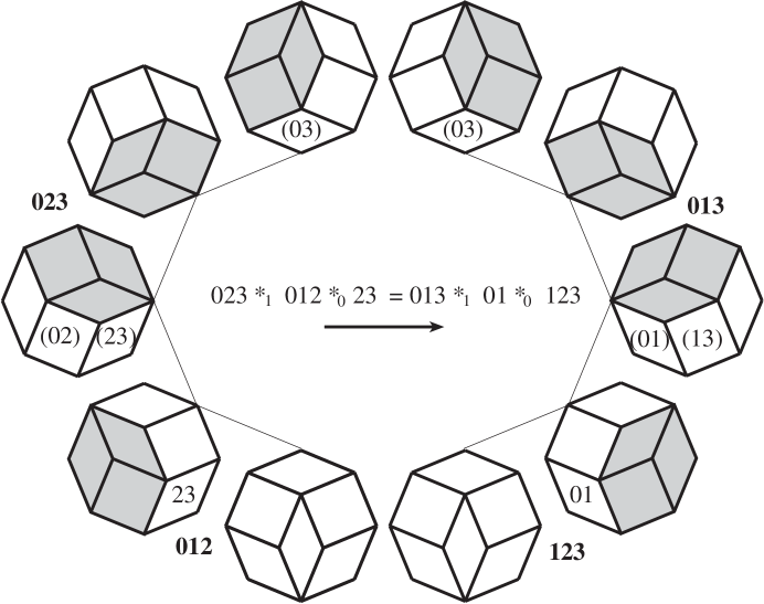
We gave diagrams indicating how the first three cocycles arise, repeating their description in block form accompanied by the geometric decomposition corresponding to the block. Note that the 2-cocycle condition can be thought of as saying “replace the interior of the hexagon on the left by the configuration on the right”. In other words, flip from the front faces to the back ones in the standard Necker cube.
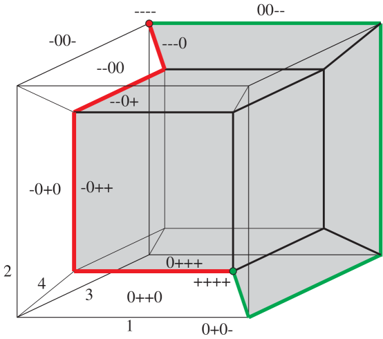
Figure 15 shows the boundary of the 4-dimensional cube, labelled by our convention. The 2-dimensional target faces are shaded, the source faces labelled, and the heavy line depicts the 1-source. To depict the 3-cocycle condition, we present the five stages of deformation of the 2-face cubes across the four 3-dimensional cubes of the 3-dimensional source faces. This corresponds to looking at the set of s arising in the respective piles. These pictures decompose as indicated in Figure 16, where the order is that determined by the corresponding block.
![[Uncaptioned image]](/html/1008.1714/assets/x35.png)
5-cube target
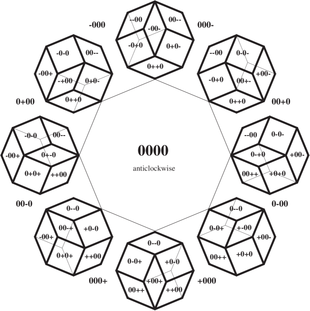
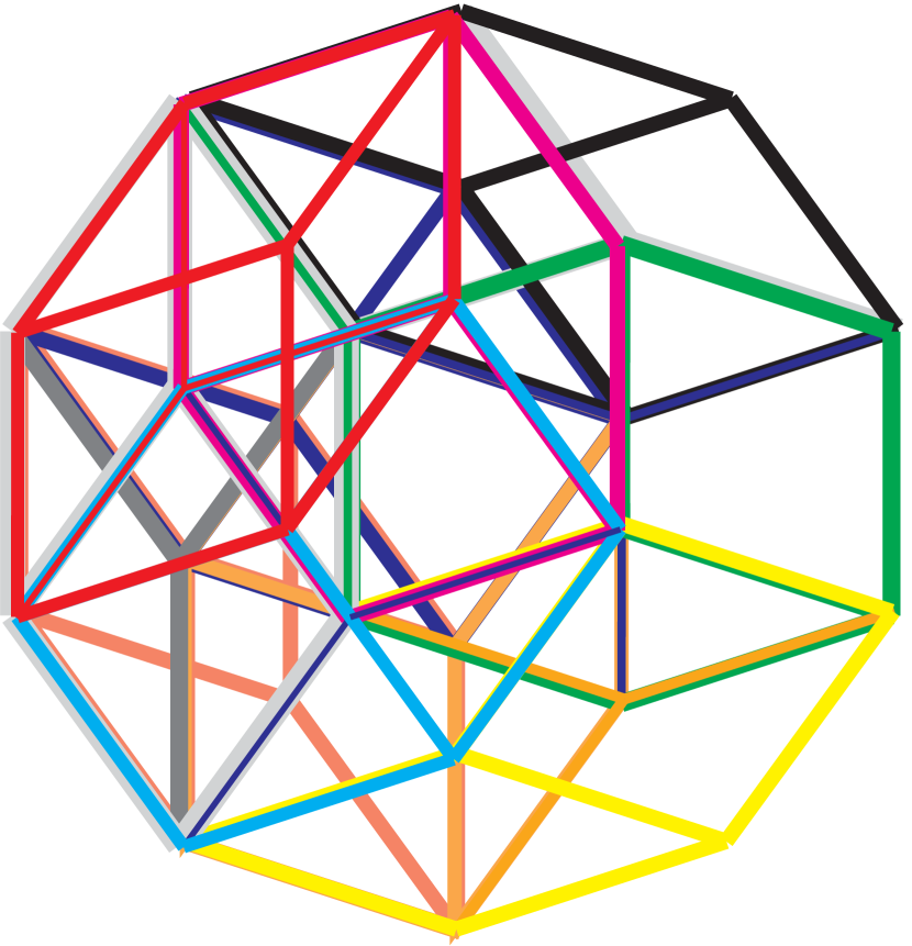
Hence if we draw the two possible paths from the 2-source to the 2-target, across the 3-source and 3-target, we obtain what we call the octagon of octagons. Note the bilateral symmetry of the figure, as well as its antipodal symmetry. If all symbols were to be deleted, the octagon of octagons shows that each figure, going clockwise around the octagon, differs from the preceding by a rotation.
In Figure 17 we show how the 3-cocycle arises from the 2-cocycle by ordering the thickenings and shiftings of cubes that occur. The left hand side of the octagon arises by considering the order of 2-cell composition for the 2-cocycle source, indicated by the numbers, and consecutively moving these across the octagon via their thickenings into 3-cubes as indicated by the bold-face hexagons. The target side of the octagon of octagons can be obtained either by symmetry considerations or by the same process.
It is clear that the unlabelled configurations of the octagon of octagons can be derived entirely without labelling any of the faces! Thus the only purpose of the labellings of the cube is to allow us to write down the cocycle conditions in a linear symbolic form, without the need for these diagrams.
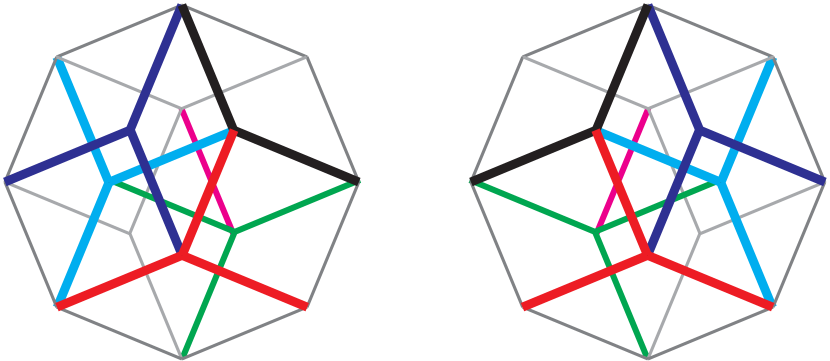
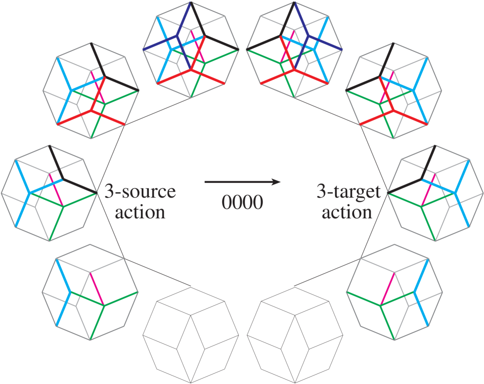
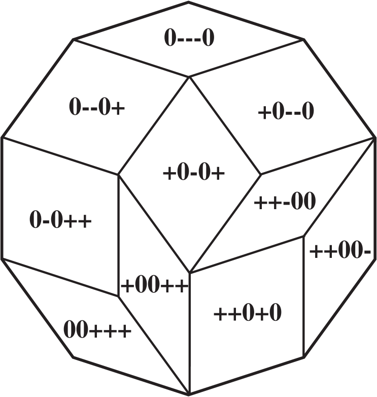
We may replace the octagon by Figure 18, which depicts the splitting of the eight s in the boundary of into the source and target sets. The octagonal “outline” we see is the union of the 1-source and 1-target, splitting the boundary 2-sphere, which itself is the union of the 2-source and 2-target, into these two hemispheres. The 3-source of is on the left, the 3-target on the right. The front faces are the 2-source , the back face . To find the upper 4 octagons of the octagon of octagons, consecutively “puncture” the s having three 2-faces exposed, thinking of the configuration as cubical soap bubbles. The order to proceed is uniquely determined at this dimensional level, and the collection of s we see at each stage gives the configurations of the octagon. We illustrate the puncturing procedure by redrawing the “octagon of octagons” as a sequence of 3-dimensional configurations of cubes.
Although it is possible to draw the “source” of the 4-cell in a single configuration – that of four cubes glued together as half of a tessaract – by doing so it is not clear how to write down a “canonical” ordering of the 2- and 3-cubes at each stage of the octagon, as a path of deformations of the 1-source to the 1-target.
= 
= 
= 
= 
= 
= 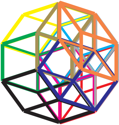
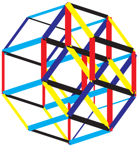
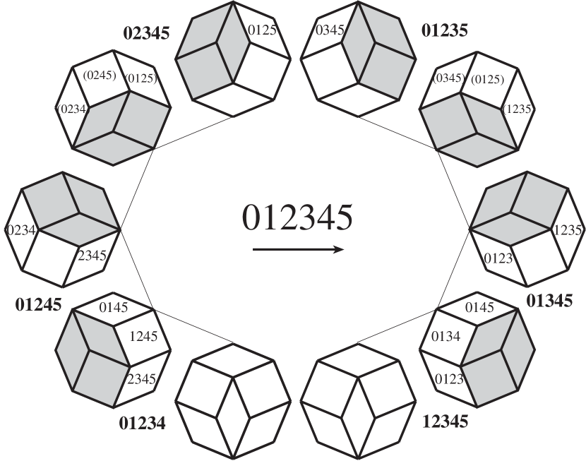
The 5-dimensional cube can be treated in the same manner. It is easiest to present the data as pictures of consecutive -collections arising in the sequence of piles. At the top and bottom of each column is and , which are again mirror images. We obtain 5 columns, corresponding to the five s of the source (Figure 19), and another 5 columns correponding to the target. Note the bilateral symmetry of the decagonal configurations for each of and , and that the configurations of are those of the source read backwards with and interchanged. Each column of decagons provides a path from to .
Between the decagons of any column we have written the word whose application transforms the decagons one to the next. Hence the shaded subsets of Figure 19 indicate for each subsequent . We merely replace the interior configuration by its mirror image, with the symbols behaving accordingly.
Each decagon itself gives a path from to . Together the five columns of either or give a path from to . In each column occurs one and six s. These latter s, together with the four of the source of , make up the ten s of the pile at that stage. The shaded s together with those remaining make up the ten of at that pile stage, accordingly giving the block structure at the 2-dimensional level, if we ignore considerations of order. From these figures we can write down a sequence of piles with their 1-dimensional sets either present or deleted.
In Figure 21, we indicate how the first four columns of arise from . We use the symbols and hatching to bring out the sub-cubes of relevance. The dotted squares correspond to the sixteen terms from the 4-cube source, depicted at the bottom. These exist in the 5-cube source as either old, new or thickened versions. The lined squares indicate thickenings. Note that one of the 4-dimensional configurations arises if we collapse all lined squares of a given decagon along the direction of the lines; each decagon arises by splitting an octagon along a path from the 0-source to the 0-target and inserting a square for each segment of the path (the lined squares). Observe that each column corresponds to doing some of the 4-dimensional operations in the “old” () copy, then moving each of the four parts of an octagon across to the “new” copy, then completing the octagon operations in the “new” () copy. The subscripts refer to the corresponding objects in 4-dimensions, with 2-dimensional source and target faces indicated accordingly.
In the sequence of figures (Figure 22 – 27) we show how the 3-faces are glued together, and how the configuration is transformed into by a sequence of modifications of the interiors of the 3-dimensional sources of the five s making up . These collections of sub-s are delineated in bold. Each copy of is replaced by a copy of , with the same 2-dimensional boundary. As with the 2-dimensional configurations, the interiors are replaced by their mirror images, the labels changing accordingly. This enables us to write down the sequence of pile sets and , but neither the order nor the intermediate stages of ’s.
8 The cubical/simplicial dichotomy
We make some remarks on the relationships between the simplicial and cubical approaches. We describe how the structure on gives rise to structure on , the -simplex, for . We shall be more detailed for the last case, deferring the others to a subsequent paper as the questions are deeper.
8.1
The ()-simplex has vertices . Each sub-simplex can be described as a word in symbols 0 and +, the presence of 0 in the position indicating that the vertex is present in the sub-simplex. Since all such words of length occur in our description of sub-cubes of the -cube, we have the standard description of as the slice off the corner of by a hyperplane.
Consider the sequence of piles occurring in the cubical cocycle condition. This gives a sequence of nested embedding of -disks into the cube, at each dimension having fixed boundary. Each pile is a collection of sets of words from , some of which do not contain ‘’. If we restrict to the subsets within the pile consisting of those sub-cubes in whose word description no ‘ occurs, we see that the action of for containing a ‘’ symbol leaves the sub-pile unaltered. Only for those consisting entirely of 0’s and +’s do we change the sub-set. Since geometrically every such intersects the slicing hyperplane in one dimension less, we see that cubical pile modifications induce a structure on the simplex also describable by piles and blocks, but where now a word in 0’s and +’s corresponds to a sub-simplex of dimension . In particular, if we look at the source and target ()-face cubes of , we pick out all ()-faces of . These are accordingly divided into two sets, the source and target faces. Note that the former correspond to the consecutive deletion of odd vertices, whereas to obtain the target faces we delete even vertices from . There is a simple procedure to derive the induced cocycle condition for from that of the cube : Rewrite according to the rules
-
1.
Starting with and proceeding down to , consider the highest dimensional cube between successive ’s.
-
2.
For each such pair, if the highest dimensional term occurring between them contains a ‘’, delete all terms between the pair, and one of the terms.
-
3.
Delete all vertices and occurrences of .
-
4.
For the words remaining, write for each occurence of 0 in the th position.
-
5.
Replace each by .
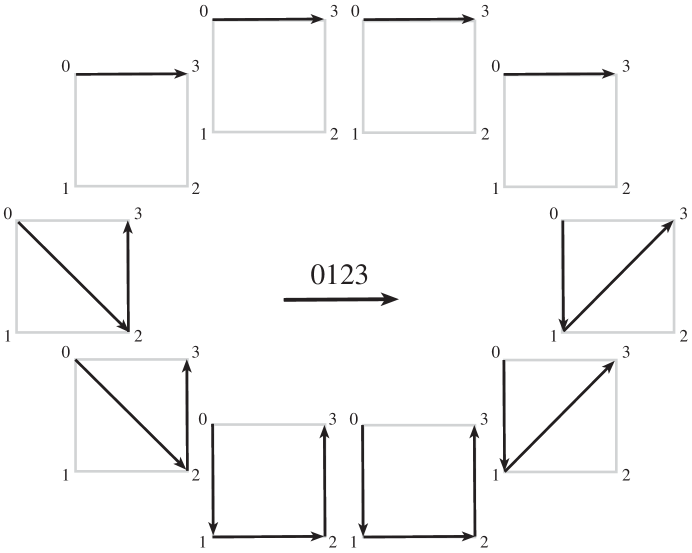
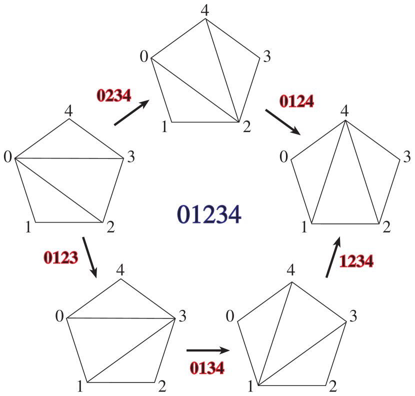
Examples 8.1: For the cocycle conditions previously described, we obtain exactly the description of simplicial cocycles obtained by Street [9]. For the 1-, 2-, 3-cubes, we obtain Figure 28. In Figure 29 we do the same for the 4-cube, the upper diagram giving the data in terms of the ‘octagon of octagons’, the lower the interpretation on the tetrahedron slice acting on paths.
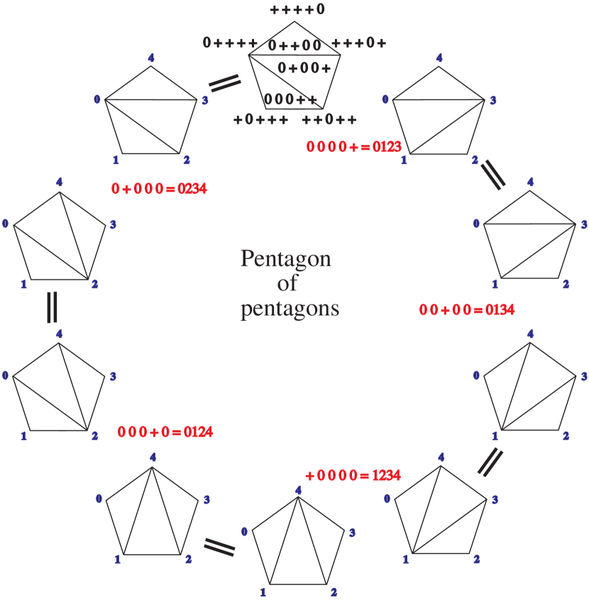
In Figure 30 we show that the 5-dimensional cube gives rise to the famous ‘pentagon of pentagons’ arising in homotopy coherence theory as well as in the definition of bicategories. We refer to [9] for further discussion. The pentagon of pentagons can be seen directly from Figures 22 – 27, by slicing the bottom of each figure with a horizontal plane. The vertices of the pentagon are determined as the intersection between the plane and the edges emanating from the 0-target of , the internal configuration of the triangles arising from intersections with s. Alternatively we can interpret the decagons as providing deformations of the 0-source of to the 0-target, each column corresponding to a configuration of triangles in . We shall shortly obtain two other derivations of the pentagon of pentagons.
In [9] the structure of an -category is shown to exist freely on the -simplex. This derives from Street’s notion of sources and targets in terms of even and odd faces. From his results on ‘excision of extremals’, it is possible to derive the cocycle conditions for this structure, non-canonically since order is not determined. Alternatively, the -category structure can be defined if we have the cocycle conditions. Since at the level of ()-faces of the -simplex we have derived the same structure as in [St], we conclude
Theorem 8.2 ([9]): (a) admits the structure of an -category.
- (b)
-
Street’s structure of orientals can be derived from the structure of oriented cubes, by slicing.
- (c)
-
There is a canonical form inductively defined for the expression of simplicial cocycle conditions.
- (d)
-
The simplicial cocycle conditions can be written in a form involving neither brackets nor the 2-categorical middle interchange law.
Roberts had conjectured that there should be a natural way of expressing the cocycle conditions without brackets.
The two approaches that follow, relating cubes and simplices, also lead to induced coycle conditions, indicating just how ‘rigid’ and canonical is the structure.
8.2 Stretching a simplex into a cube
We show how the cocycle condition on gives rise to one on . To do this we briefly describe how to ‘stretch’ the -simplex into a cube.
-
1.
For dimension one, and coincide.
-
2.
Higher dimensional simplices arise by ‘coning’, whereas cubes arise by taking the product with , the unit interval. We use labellings of vertices of simplices by the symbols . For the 1-simplex, vertices and (Figure 31), the 1-cell is labelled .
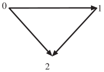
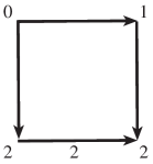
Figure 31: Expanding a labeled 2-simplex into a labeled 2-cube 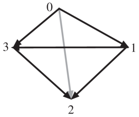
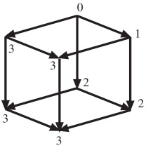
Figure 32: Expanding a labeled 3-simplex into a labeled 3-cube Take the 2-cube whose other two vertices are labelled ‘2’. The edges are now , , , and ‘’. The latter edge is really a stretched out vertex, corresponding to an ‘identity arrow’ in the categorical setting. Note that if we identify everything labelled ‘2’ together, we obtain a triangle (2-simplex).
-
3.
Taking the product with the interval, and labelling all new vertices by ‘3’ leads to the 3-cube labelled as in Figure 32. Again, collapsing together like-labelled objects yields the tetrahedron. The source and target configurations for the 3-cube yield Figure 33, in which each 2-cell is labelled by its vertices. We obtain the simplicial 2-cocycle condition from the cubical one by direct substitution, deleting degenerate ( identity) cells. Note that the only change from the source to the target configuration is the internal shape and re-labelling of the vertex.
Figure 33: The 3-cubical 2-cocycle becomes the 3-simplicial 2-cocycle 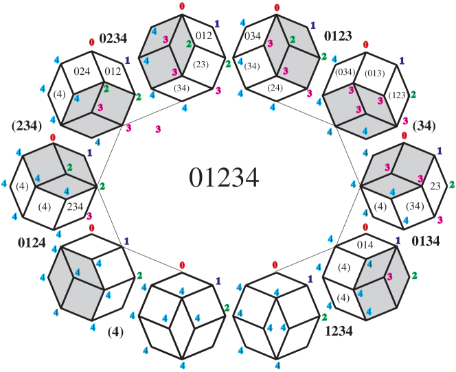
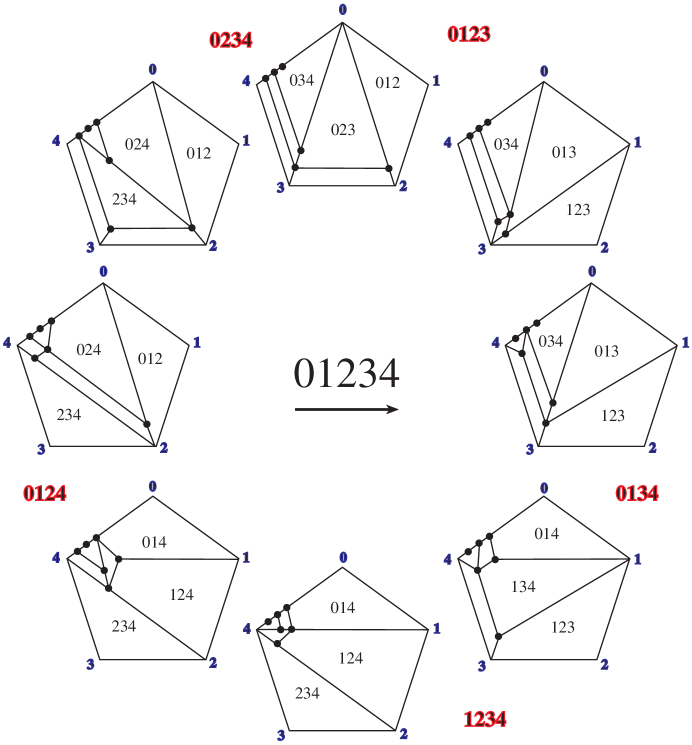
Figure 34: Deriving the pentagon of pentagons from the octagon of octagons -
4.
Proceed in the same way to obtain ‘exploded’ into .
-
5.
The rule to reverse the process is to replace a vertex of the cube, as a word in and , by the position of the highest occurring , or if none occur. For an arbitrary word in , or , we also record all positions of beyond the highest . This enables us to relabel each sub-cube as an exploded sub-simplex.
-
6.
Now rewrite cubical cocycles by replacing words in this fashion, forgetting those (as in of the slicing approach) correponding to ‘identities’. These identities are those simplices of dimension less than the cube from which they arise in this correspondence.
In Figure 34, we show how the octagon of octagons gives rise directly to the pentagon of pentagons. The upper figure gives direct substitution, the lower a deformation of the figures into a more recognisable shape.
The cubes arising in this fashion have a number of faces which are ‘identities’. The same happens in the following procedure:
8.3 Strings on simplices
Any (ordered) path from to on is uniquely determined by listing the vertices through which it passes. Since the list for any such path contains and , we need not include these in a specification of the path. If we insist on listing vertices in increasing order of magnitude, and and are two consecutive integers in the list with , then for each triangle with there is a triangle in the -simplex and a new path obtained by including . In this way triangles act on paths, and thus label morphisms in the (discrete) space of paths.
The resulting complex, with paths as objects and triangles as morphisms (acting as deformations of one path to another), is well known to form . We refer the reader to [3] or [7]. Not all faces of the cube correspond to faces of the simplex, some as in the previous procedure corresponding to ‘identities’. There is fortunately a well defined procedure to see which sub-cubes correspond to sub-simplices. Some repetitions occur, as can be understood by considering the effect of a triangle on a path: different paths may abut the same triangle, giving rise to distinct vertices of the cube, but with edges emanating having the same triangular correspondence. The application of this approach to the understanding of simplicial oriental cocycles was initiated by Duskin [4].
Here is the prescription for converting the cubical ()-cocycle condition into the simplicial ()-cocycle condition:
-
1.
Consider terms of dimension . A unique such occurs between consecutive ’s.
-
2.
If any ’s in the word are separated by a , delete all terms between the prior and subsequent . Delete one of the ’s.
-
3.
If no occurs before a , write .
-
4.
If a occurs before a , record the highest position in which a occurs before a is encountered.
-
5.
Record all positions in which a occurs.
-
6.
If no is then reached before the end of the word, write .
-
7.
If a does occur to the right of all ’s, record the position of the first such encountered.
-
8.
Now look at -dimensional words between the , and follow the analogues of steps (2) and (3).
-
9.
Repeat this process for every dimensional word.
-
10.
Replace each by .
-
11.
Insert the terms before the word, if the first number of a word is . If the last letter is , add after the word the symbols
Examples 8.3: In Figures 35 and 36 we show again how the usual simplicial cocycle conditions arise. From the 3-cube we obtain the pentagon of pentagons, from which it is also possible to see that the ‘identity’ face of the 3-cube correponds to a re-ordering of the triangles across which we are deforming the 1-source of onto the 1-target. Hence the cube contains some additional information about structure manifest at the simplicial level.
It is possible to iterate this procedure, and consider strings on the cube. Doing so leads to the parallelahedra, which in dimensions 2- and 3- are the hexagon and truncated octahedron. The parallelahedra are known to tesselate Euclidean space, and like the cube and simplex have an intimate relationship with the symmetric groups. We refer the reader to Baues [3] for applications to the geometric cobar construction. Another discussion occurs in Leitch [7]. We also remark that to carry over to the parallelahedra the -category structures discussed above should be possible in a geometric fashion, there being an inductive definition for the construction of parallelahedra. This is more difficult to describe directly as the parallelahedra are no longer regular figures. A categorical approach should exist.
These descriptions for obtaining simplicial cocycles from cubical ones show that the cubical and simplicial cocycles/structures are deeply interlocked. The procedures ‘take strings’, ‘slice’ and ‘explode’ provide a sequence of correspondences of structures: three modifications from each of the -cubical cocycles, and three ways to obtain each of the -simplicial cocycles:
There is an analogue of the ‘-blocks’ for cubes in the simplicial context, and a manifestation of the symmetries of the cubical cocycles. On the other hand, the three relationships described above show how the structure on the cubes gives rise to a structure on simplices, but it is not clear how the procedure can be reversed for any of the approaches!
It would be of interest to investigate further the commutativity of the above sequences, with respect to face and degeneracy maps for cubes or simplices. In fact, to put the whole structure in a more explicitly categorical framework would be desirable. The symmetries of many of the objects also suggests possible extensions of Connes’ cyclic homology, for which we refer to Goodwillie [5] for a categorical approach.
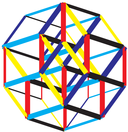
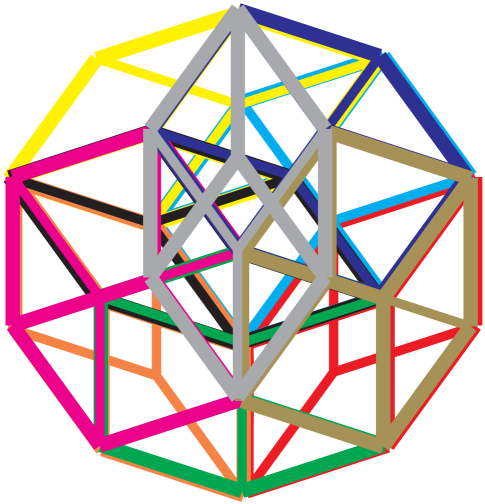
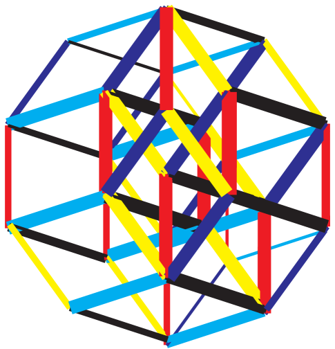
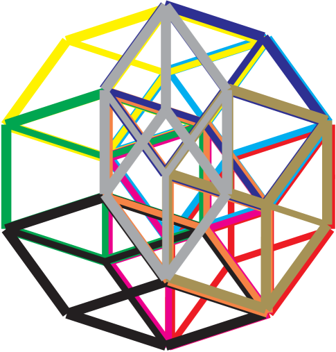
Added 2009: 3-cell recombination for the 5-cube [5], figures after references
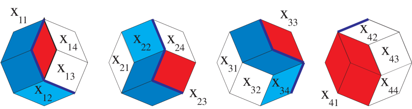
The 3-source of the 5-cube [5] contains 3-cubes. Each cube is a parallel class determined by the location of three 0’s in a string of length 5, there being possibilities in total corresponding to the remaining entries. An application of a 4-cube in the 5-cube 4-source may change the representative: each 3-cube class is involved twice in changing the two entries to corresponding to the 3-cubes in the 3-target, which are the first and last colummns. We only record the position of 0’s in intermediate columns.
Each column bold indicates source 3-cubes of the operational 4-cube: Observe that in each case reordering can be achieved before application, so that these source 3-cubes occur consecutively. Partial order rearrangement is possible when two 3-cubes do not share a common face (pair of numbers): two cubes intersect on at most 1 vertex. (This is clearer in the dual Pascal’s triangle version). The columns before the double vertical lines, read from bottom to top, enable the filling of the 3-ball by 10 distinct 3-cubes.
The following figures, from the original, indicate how the simplicial cocycle from the 6-simplex derives from the 5-cube: three nontrivial columns occur in the 5-cube source, and four in the target. Observe from the first 5-cube source column the four- and five-simplices, or considering only source four-simplices:
which are the labeled 2-cells in of Street [9]. Adding in the cubically-ordered listed three-simplices gives
References
- [1] I.R.Aitchison, The Geometry of Oriented Cubes, Macquarie University Research Report No: 86-0082, 1986.
- [2] added 2009 I.R.Aitchison, String diagrams for non-abeIian cocycle conditions, Louvain-la-Neuve Category Theory Conference, 1987.
- [3] H.J. Baues, Geometry of loop spaces and the cobar construction, Memoirs of the American Math. Soc., #230 May 1980.
- [4] J. Duskin, handwritten notes, 1983/1984.
- [5] T.M. Goodwillie, Cyclic homology, derivations and the free loop space, Topology 24 (1985) 187-215.
- [6] G.M. Kelly and Ross Street, Review of the elements of 2-categories, Lecture Notes in Math. 420 (Springer-Verlag, Berlin-Heidelberg-New York, 1974) 75-103.
- [7] R.D. Leitch, The homotopy commutative cube, J. London Math. Soc., (2) (1974) 23-29.
- [8] John E. Roberts, Mathematical aspects of local cohomology, Proceedings of the Colloquium on Operator Algebras and their Application to Mathematical Physics, (Marseille 1977).
- [9] Ross Street, The algebra of oriented simplices, J. Pure Appl. Algebra 49 (1987), 283-335.
- [10] added 2009 Ross Street, Higher Categories, Strings, Cubes and Simplex Equations, Applied Categorical Structures 3: 29-77, 1995. John Myhill Memorial Lectures at the State University of New York, Buffalo, 20–23 April 1993.
![[Uncaptioned image]](/html/1008.1714/assets/x248.png)
![[Uncaptioned image]](/html/1008.1714/assets/x249.png)
![[Uncaptioned image]](/html/1008.1714/assets/x250.png)
![[Uncaptioned image]](/html/1008.1714/assets/x251.png)
![[Uncaptioned image]](/html/1008.1714/assets/x252.png)
![[Uncaptioned image]](/html/1008.1714/assets/x253.png)
![[Uncaptioned image]](/html/1008.1714/assets/x254.png)
![[Uncaptioned image]](/html/1008.1714/assets/x255.png)
![[Uncaptioned image]](/html/1008.1714/assets/x256.png)
![[Uncaptioned image]](/html/1008.1714/assets/x257.png)
![[Uncaptioned image]](/html/1008.1714/assets/x258.png)
![[Uncaptioned image]](/html/1008.1714/assets/x259.png)
![[Uncaptioned image]](/html/1008.1714/assets/x260.png)
![[Uncaptioned image]](/html/1008.1714/assets/x261.png)
![[Uncaptioned image]](/html/1008.1714/assets/x262.png)
![[Uncaptioned image]](/html/1008.1714/assets/x263.png)
![[Uncaptioned image]](/html/1008.1714/assets/x264.png)
![[Uncaptioned image]](/html/1008.1714/assets/x265.png)
![[Uncaptioned image]](/html/1008.1714/assets/x266.png)