Tailorable couplings of a cantilever with a superconducting charge qubit:
Quantum state engineering

Abstract

We propose a theoretical scheme to realize tailorable couplings between a cantilever and a superconducting charge qubit. By tuning the controllable parameters of the qubit, both linear and nonlinear couplings between the cantilever and the qubit can be achieved. Based on these couplings, we show the preparation of the cantilever into some interesting quantum states, such as superposed coherent states and squeezed states, via manipulating and detecting the qubit. We also study the influence of the environment on quantum states of the cantilever. It is indicated that decoherence induced by the environment can drive the cantilever from superposed coherent states into the steady coherent state. It is also found that the environment can induce the steady-state position squeezing of the cantilever under a critical temperature. These results will shed new light on production of nonclassical effects of the cantilever.

I Introduction

As is well known, it is of very significance to couple a mechanical object to an electronic system since the electronics may be used to measure the quantum nature of the mechanical object while quantum effects in electronic systems may be measured by mechanics. Cantilevers, as important components of magnetic resonance force microscopy (MRFM) Sidles1995 ; Mamin2003 ; Bermangroup , have attracted much attention of both theorists and experimentalists in many fields of physics such as condensed matter physics and quantum information science Cleland2003 ; Blencowe2004 ; Schwab2005 . For example, MRFM has been recently proposed as a qubit readout device for spin-based quantum computers DiVincenzo1995 ; Berman2000 . As one kind of nanomechanical resonators, the cantilever can also be used as a platform to study some fundamental problems in quantum mechanics such as quantum measurement Schwab2004 , quantum decoherence Zurek1991 , the boundary between quantum and classical communities Katz2007 , and test of quantum mechanics in macroscopic scales Armour2002 ; Bouwmeester2003 . By far, with the high-speed development of modern micro-fabrication techniques, the preparation of nanomechanical resonators with high frequency and high quality factor  Knobel2003 ; Huang2003 ; Gaidarzhy2005 has become possible. At the same time, efficient cooling technologies  Imamoglu2004 ; Karrai2004 ; Zhang2005 ; Naik2006 ; Zeilinger2006 ; Heidmann2006 ; Bouwmeester2006 ; Poggio2007 ; Wilson2007 ; Marquardt2007 ; Xue2007B ; Yi2008 ; Wang2009 ; Ouyang2009 drive nanomechanical resonators approaching quantum realm. Therefore, it is expected to observe quantum evidences Quantumevidence in nanomechanical resonators such as cantilevers. As a precondition, it is an interesting topic that how to generate some nonclassical states  Xue2007A ; Liao2008 ; Jacobs2007 ; Siewert2005 ; Tian2005 ; Rabl2004 ; Ruskov2005 ; Zhou2006 ; Zhang2009 ; Hou2007 ; Buks2007 ; Eisert2004 ; Bos2005 ; Vitali2007 such as Fock states, superposed states, squeezed states, and entangled states in cantilevers. In addition, from the viewpoint of MRFM, cantilevers play the role of probers to read out the states of a single spin, therefore the preparation of cantilevers into some states with position squeezing can improve the measurement precision Scully1997 .

For manipulation of the vibrational states of nanomechanical resonators, many schemes have been proposed by coupling nanomechanical resonators with various physical systems such as superconducting qubits  Armour2002 ; Irish2005 ; Schwab2009 ; Sun2006 ; Xue2007C , superconducting transmission line resonators  Blencowe2007 ; Rocheleau2009 ; Hertzberg2009 , cold ions, atoms and molecules  Tian2004 ; Treutlein2007 ; Treutlein2010 ; Meystre2010 , and quantum dots  Liao2008 ; Lambert2008 ; Lambert2008B ; Bennett2010 . These considered physical systems play the role of indirectly assistant controller Jacobs2007B . Therefore, they should be of well controllability and readability. For example, during the latest decade, great advances in quantum information processing based on superconducting charge qubits have been made Makhlin2001 ; You2005 . It has been shown that superconducting charge qubits have well controllability and readability Nakamura1999 . Stimulated by these, in this paper, we propose a new scheme to couple a cantilever with a superconducting charge qubit Makhlin1999 . We can manipulate the cantilever through tuning and measuring the qubit as an indirect controller. Both linear and nonlinear couplings Zhou2006 between the cantilever and the qubit can be obtained. Especially, we emphasize that the obtained nonlinear-type coupling for a cantilever is one of the main results in this work. Based on these couplings, we show how to create superposed coherent states and squeezed states of the cantilever by manipulation of the qubit. The preparation of superposed coherent states shows the appearance of quantum superposition in the cantilever. And the squeezing in the cantilever not only shows nonclassical evidence but also has wide potential for practical application.

This paper is organized as follows. In Sec. II, we introduce the physical model and present correspondent Hamiltonian. In Sec. III, we show how to generate superposed coherent states of the cantilever, and investigate the influence of decoherence induced by environment on superposed coherent states of the cantilever. In Sec. IV, we show how to obtain a dynamical squeezing of the cantilever, especially it is indicated that there exists a steady-state position squeezing. We conclude this paper with some discussions in the last section. Finally, we present two Appendixes A and B for derivation of evolution equations of the cantilever in an environment.

II Physical model and Hamiltonian

We start with introducing the physical setup as illustrated in Fig. 1, a cantilever is fabricated above a superconducting charge qubit which is formed by an SQUID-based Cooper-pair box Makhlin1999 .

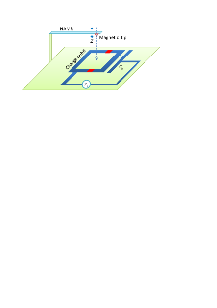
Figure 1: (Color online) Setup of a cantilever mounted with a magnetic tip coupling with an SQUID-based charge qubit. The magnetic field generated by the magnetic tip threads through the superconducting loop of the charge qubit. Since the generated magnetic field depends on the vibration amplitude $z$ of the cantilever, and the magnetic flux in the loop is a controllable parameter of the qubit, therefore a coupling between the cantilever and the qubit is induced.

A ferromagnetic particle mounted on the cantilever tip produces a magnetic field Xue2007

$$B_{\textrm{tip}}=\frac{\mu_{0}}{4\pi r^{3}}\left[3\left(\vec{n}\cdot\vec{m}\right)\vec{n}-\vec{m}\right],$$ (1)

threading the superconducting loop of the qubit, where $\mu_{0}$ is the vacuum magnetic conductance, $\vec{n}$ is the unit vector pointing to the direction from the tip to the center of the loop. Here we assume that the magnetic tip is right on top of the center of the loop. The vector $\vec{m}$ is the magnetic moment of the magnetic tip pointing to the $z$ direction, and $r$ is the distance between the tip and the center of the loop. For a tiny vibration of the cantilever, the magnetic field threading the loop of the qubit can be approximated as

$$B_{\textrm{tip}}\approx B_{0}-Cz,$$ (2)

where $B_{0}=\mu_{0}m/(2\pi r^{3})$ and $C=3\mu_{0}m/(2\pi r^{4})$ with $m=|\vec{m}|$. Since the generated magnetic field depends on the position $z$, then couplings between the cantilever and the qubit can be induced as follows: The vibration of the cantilever leads to a change of the magnitude for the magnetic field threading the loop of the qubit. As a result, the corresponding magnetic flux will be changed. At the same time, since the magnetic flux is a controllable parameter of the qubit, therefore the vibration can induce a coupling between the cantilever and the qubit.

As for the SQUID-based charge qubit Makhlin1999 , its Hamiltonian reads

$$H_{q}=4E_{C}\left(n_{g}-\frac{1}{2}\right)\sigma_{z}-E_{J}\cos\left(\frac{\pi\Phi_{e}}{\Phi_{0}}\right)\sigma_{x},$$ (3)

where $E_{C}=e^{2}/[2(2C_{J}+C_{g})]$ is the single-electron charging energy, $C_{J}$ and $C_{g}$ are, respectively, the capacitances of each Josephson junction and the gate capacitance in the qubit; $n_{g}=C_{g}V_{g}/2e$ is the gate charge number with $V_{g}$ being gate voltage; $E_{J}$ is the Josephson coupling energy; $\Phi_{e}$ and $\Phi_{0}$ are the externally biasing flux and flux quanta, respectively. The Pauli operators introduced in Eq. (3) are defined by

$$\sigma_{z} = |0\rangle\langle 0|-|1\rangle\langle 1|,\hskip 14.22636pt\sigma_{x}=|0\rangle\langle 1|+|1\rangle\langle 0|,$$ (4)

where the states $|0\rangle$ and $|1\rangle$ represent that there is no and one extra cooper pair on the inland, respectively.

We consider a case that the externally biasing magnetic flux $\Phi_{e}$ is composed of two parts. One is generated by the magnetic tip, and the other is generated by an externally controllable electric current. We can express the total biasing magnetic flux as $\Phi_{e}=(B_{\textrm{tip}}+B_{x})S$, where $B_{x}$ is the magnetic field generated by the externally controllable electric current, $S$ is the area of the superconduting loop. For a tiny vibration, the cantilever can be modeled as a quantum harmonic oscillator, which is depicted by the usual Bosonic creation and annihilation operators $a^{\dagger}$ and $a$, satisfying the commutative relation $[a,a^{\dagger}]=1$. Then the magnetic field generated by the magnetic tip can be expressed as

$$B_{\textrm{tip}}\approx B_{0}-Cz_{0}(a^{\dagger}+a),$$ (5)

where $z_{0}=1/\sqrt{2\mu\omega}$ (with $\hbar=1$) is zero-point uncertainty for the ground state of the cantilever, $\mu$ and $\omega$ are the mass and frequency of the cantilever, respectively.

The Hamiltonian of the total system including the cantilever and the charge qubit reads

$$H=\frac{\omega_{0}}{2}\sigma_{z}+\omega a^{\dagger}a-E_{J}\cos[\phi_{0}+\phi(a^{\dagger}+a)]\sigma_{x},$$ (6)

where $\omega_{0}=8E_{C}(n_{g}-1/2)$ and $\omega$ are, respectively, the frequencies of the qubit and the cantilever. We also introduce two parameters

$$\phi_{0}=\pi S(B_{0}+B_{x})/\Phi_{0},\hskip 14.22636pt\phi=-\pi SCz_{0}/\Phi_{0}.$$ (7)

Hamiltonian (6) obviously shows a nonlinear coupling between the cantilever and the charge qubit. A coupling of similar form between a bosonic mode and a two-level system has been obtained in a trapped-ion system Monroe2005 . A recent scheme has been proposed to obtain a nonlinear interaction between a doubly-clamped beam and a superconducting charge qubit Zhou2006 . However, the method proposed in Ref. Zhou2006 is not valid for a cantilever.

Hamiltonian (6) is very useful in quantum information processing. Many useful interactions can be tailored from Eq. (6) by choosing proper parameters. For example, we tune the externally controllable current such that $\cos\phi_{0}=0$, then Eq. (6) becomes

$$H_{1}=\omega a^{\dagger}a+\frac{\omega_{0}}{2}\sigma_{z}+E_{J}\sin[\phi(a^{\dagger}+a)]\sigma_{x},$$ (8)

which can be reduced to the well-known Jaynes-Cummings Hamiltonian without rotating wave approximation

$$H_{1}\approx\frac{\omega_{0}}{2}\sigma_{z}+\omega a^{\dagger}a+g(a^{\dagger}+a)\sigma_{x},$$ (9)

by expanding the sine function up to the first order of parameter $\phi$, where we introduce the coupling strength $g=E_{J}\phi$.

On the other hand, if we choose the external magnetic flux to ensure $\cos\phi_{0}=1$, then Eq. (6) reduces to

$$H_{2}=\omega a^{\dagger}a+\frac{\omega_{0}}{2}\sigma_{z}-E_{J}\cos[\phi(a^{\dagger}+a)]\sigma_{x},$$ (10)

which can be further simplified by expanding the cosine function up to the second order of $\phi$,

$$H_{2}\approx\omega a^{\dagger}a+\frac{\omega_{0}}{2}\sigma_{z}-E_{J}\sigma_{x}-g^{\prime}(a^{\dagger}+a)^{2}\sigma_{x},$$ (11)

where $g^{\prime}=E_{J}\phi^{2}/2$ is a nonlinear coupling strength between the cantilever and the qubit. These two kinds of couplings given in Eqs. (9) and (11) are very useful in quantum optics and quantum information processing. As examples, in the following two sections, we will study quantum state engineering based on these couplings.

III Preparation of superposed coherent states

Superposed coherent states are typical quantum states which exhibit nonclassical properties. In this section, we show how to prepare the cantilever into superposed coherent states with the above obtained Hamiltonian (9). We also study the decoherence of the created superposed coherent states when the cantilever is subjected to an environment.

III.1 Generation of superposed coherent state

Firstly, we consider an ideal situation in which there is no dissipation for the cantilever. Since the state preparation can be realized in a very short time interval, it is reasonable to neglect the dissipation during the state preparation process. We tune the gate voltage $V_{g}$ such that $n_{g}=1/2$, that is $\omega_{0}=0$, then Eq. (9) reduces to the conditional displacement harmonic oscillator (CDHO) Hamiltonian

$$H_{\textrm{CDHO}}=\omega a^{\dagger}a+g(a^{\dagger}+a)\sigma_{x}.$$ (12)

Corresponding to the qubit in states $|\pm\rangle$, the displacement terms are $\pm g(a^{\dagger}+a)$, respectively, where states $|\pm\rangle$ are the eigenstates of Pauli operator $\sigma_{x}$, with the respective eigenvalues $\pm 1$.

For generation of superposed coherent states, we suppose the total system consisting of the cantilever and the qubit is initially prepared in a state $|\varphi(0)\rangle=|\alpha_{i}\rangle\otimes|0\rangle_{q}$, where $|\alpha_{i}\rangle$ is the usual Glauber coherent state, which is defined as the eigenstate of annihilation operator $a$, i.e., $a|\alpha_{i}\rangle=\alpha_{i}|\alpha_{i}\rangle$, and $|0\rangle$ is defined by $|0\rangle=(|+\rangle+|-\rangle)/\sqrt{2}$. Making use of Hamiltonian (12), the state of the total system at time $t$ is

$$|\varphi(t)\rangle = \exp\left(-itH_{\textrm{CDHO}}\right)|\varphi(0)\rangle$$ (13)

$$= \frac{1}{2}\left[\left(e^{i\theta_{+}}|\alpha_{+}\rangle+e^{i\theta_{-}}|\alpha_{-}\rangle\right)|0\rangle\right.$$

$$\left.+\left(e^{i\theta_{+}}|\alpha_{+}\rangle-e^{i\theta_{-}}|\alpha_{-}\rangle\right)|1\rangle\right],$$

where we introduce the parameters

$$\alpha_{\pm} =\alpha_{i}e^{-i\omega t}\pm\frac{g}{\omega}(e^{-i\omega t}-1),$$ (14a)

$$\theta_{\pm} =\frac{g}{\omega}\left[gt-\left(\frac{g}{\omega}\pm\alpha_{i}\right)\sin(\omega t)\right].$$ (14b)

During the derivation of Eq. (13), we have used the following formula Liao2007 ,

$$e^{[\theta(\beta_{1}a+\beta_{2}a^{{\dagger}}a+\beta_{3}a^{{\dagger}})]}=e^{f_{1}a^{{\dagger}}}e^{f_{2}a^{{\dagger}}a}e^{f_{3}a}e^{f_{4}}$$ (15)

with

$$f_{1} =\beta_{3}\left(e^{\beta_{2}\theta}-1\right)/\beta_{2},$$ (16a)

$$f_{2} =\beta_{2}\theta,$$ (16b)

$$f_{3} =\beta_{1}\left(e^{\beta_{2}\theta}-1\right)/\beta_{2,}$$ (16c)

$$f_{4} =\beta_{1}\beta_{3}\left(e^{\beta_{2}\theta}-\beta_{2}\theta-1\right)/\beta_{2}^{2}.$$ (16d)

The action of the operator given in Eq. (15) on a coherent state $|\alpha_{i}\rangle$ yields Liao2007 :

$$e^{[\theta(\beta_{1}a+\beta_{2}a^{{\dagger}}a+\beta_{3}a^{{\dagger}})]}|\alpha_{i}\rangle=e^{\varepsilon}\left|f_{1}+\alpha_{i}e^{f_{2}}\right\rangle,$$ (17)

where $\varepsilon$ is given by the following expression

$$\varepsilon = f_{4}+f_{3}\alpha_{i}+\left(|\alpha_{i}\exp(f_{2})|^{2}-|\alpha_{i}|^{2}+|f_{1}|^{2}\right.$$ (18)

$$\left.+2\textrm{Re}[f_{1}\alpha_{i}^{*}\exp(f_{2}^{*})]\right)/2.$$

From Eq. (13), it is obvious to prepare the cantilever into superposed coherent states through measuring the qubit. Corresponding to the states $|0\rangle$ and $|1\rangle$ of the qubit are measured, the cantilever collapses to the following superposed coherent states

$$|\psi_{\pm}\rangle=\mathcal{N}_{\pm}\left(e^{i\theta_{+}}|\alpha_{+}\rangle\pm e^{i\theta_{-}}|\alpha_{-}\rangle\right),$$ (19)

where $\mathcal{N}_{\pm}^{-2}=2\{1\pm\textrm{Re}[\exp(-i(\theta_{+}-\theta_{-}))\langle\alpha_{+}|\alpha_{-}\rangle]\}$ are normalization constants.

For a special case, we suppose the cantilever is initially prepared in a vacuum state, i.e., $\alpha_{i}=0$, then the states of the cantilever at time $t$ are the so-called Schrödinger cat states Gerry

$$|\varphi_{\pm}\rangle=\mathcal{M}_{\pm}\left(|\beta\rangle\pm|-\beta\rangle\right),$$ (20)

with $\beta=g[\exp(-i\omega t)-1]/\omega$ and $\mathcal{M}_{\pm}^{-2}=2[1\pm\exp(-2\beta^{2})]$.

When the qubit is detected in states $|0\rangle$ or $|1\rangle$, the coupling term $g(a^{\dagger}+a)\sigma_{x}$ between the qubit and the cantilever will entangle them. Therefore, from the experimental viewpoint, we should decouple the cantilever and the qubit, as long as the superposed coherent states are prepared. The method to decoupling is making the second measurement on the qubit in states $|\pm\rangle$. Since states $|\pm\rangle$ are eigenstates of the operator $\sigma_{x}$, then the qubit will stay in states $|\pm\rangle$ forever, and the dynamics of the cantilever is governed by the displaced harmonic oscillator (DHO) Hamiltonian

$$H_{\textrm{DHO}}=\omega a^{\dagger}a+g_{s}(a^{\dagger}+a),$$ (21)

where $g_{s}=\pm g$ corresponding to the qubit in states $|\pm\rangle$.

III.2 Decoherence of superposed coherent states

In this subsection, we investigate the decoherence of superposed coherent states produced in the previous subsection. As a practical physical system, the cantilever couples inevitably with its external environment. Therefore, the cantilever prepared in superposed coherent states will loss its coherence and energy. We suppose that the preparation time for this initial state is very short, thus we neglect the decoherence in the course of the initial state preparation process.

The dynamics of the cantilever is governed by the quantum master equation

$$\dot{\rho}=i[\rho,H_{\textrm{DHO}}]+\mathcal{L}[\rho],$$ (22)

where the decoherence of the cantilever is phenomenologically represented by the superoperator $\mathcal{L}$. At a temperature of $T$, this superoperator can be written as Scully1997

$$\mathcal{L}[\rho] = \frac{\gamma}{2}(\bar{n}_{th}+1)(2a\rho a^{\dagger}-a^{\dagger}a\rho-\rho a^{\dagger}a)$$ (23)

$$+\frac{\gamma}{2}\bar{n}_{th}(2a^{\dagger}\rho a-aa^{\dagger}\rho-\rho aa^{\dagger}),$$

where $\gamma$ is decay rate, and $\bar{n}_{th}=1/[\exp(\omega/T)-1]$ is average thermal excitation number of the thermal bath at frequency $\omega$. Equation (22) shows that there are three kinds of actions on the cantilever. The free Hamiltonian $\omega a^{\dagger}a$ rotates the system in phase space. The driving term $g_{s}(a^{\dagger}+a)$ displaces the cantilever in phase space. And the dissipation term $\mathcal{L}$ decreases the coherence and energy of the system.

To see the evolution of the cantilever, we need to solve quantum master equation (22). In order to do this, we introduce the following transform,

$$\rho^{(2)}(t) =D^{\dagger}(\alpha(t))R^{\dagger}(\theta(t))\rho(t)R(\theta(t))D(\alpha(t)),$$ (24a)

$$R(\theta(t)) =\exp(-i\theta(t)a^{\dagger}a),$$ (24b)

$$D(\alpha(t)) =\exp(\alpha(t)a^{\dagger}-\alpha^{\ast}(t)a),$$ (24c)

with

$$\theta(t) =\omega t,$$ (25a)

$$\alpha(t) =\frac{ig_{s}}{\frac{\gamma}{2}+i\omega}\left(e^{-\frac{\gamma t}{2}}-e^{i\omega t}\right),$$ (25b)

then quantum master equation (22) can be transformed to a standard form

$$\dot{\rho}^{(2)} = \frac{\gamma}{2}(\bar{n}+1)(2a\rho^{(2)}a^{\dagger}-a^{\dagger}a\rho^{(2)}-\rho_{s}^{(2)}a^{\dagger}a)$$ (26)

$$+\frac{\gamma}{2}\bar{n}(2a^{\dagger}\rho^{(2)}a-aa^{\dagger}\rho^{(2)}-\rho^{(2)}aa^{\dagger}),$$

which describes the evolution for a harmonic oscillator in a heat bath. The detailed derivation of quantum master equation (26) will be presented in Appendix A.

The operators $R(\theta)$ and $D(\alpha)$ in Eq. (24) are, respectively, the usual rotation and displacement operators for a harmonic oscillator in phase space. In principle, the solution for quantum master equation (26) can be obtained with the superoperator method. However, for simplicity, we only give the analytical solutions for the zero temperature case in the following.

Based on the above discussions, the dynamical evolution of the cantilever can be obtained as follows: When the cantilever is initially prepared in an initial state $\rho(0)$, then the state $\rho(t)$ of the cantilever at time $t$ can be obtained through the processes

$$\rho(0)\rightarrow\rho^{(2)}(0)\rightarrow\rho^{(2)}(t)\rightarrow\rho(t).$$ (27)

The two processes $\rho(0)\rightarrow\rho^{(2)}(0)$ and $\rho^{(2)}(t)\rightarrow\rho(t)$ are determined by the transform given in Eq. (24) and its inverse transform, and the evolution process $\rho^{(2)}(0)\rightarrow\rho^{(2)}(t)$ is governed by quantum master equation (26) in the transformed representation.

We assume that the initial state of the cantilever is

$$\left|\psi\left(0\right)\right\rangle=\mathcal{N}_{\varphi}\left(\left|\beta\right\rangle+e^{i\varphi}\left|-\beta\right\rangle\right),$$ (28)

where $\mathcal{N}_{\varphi}=[2(1+\exp(-2\beta^{2})\cos\left(\varphi\right))]^{-1/2}$ is the normalization constant. Then the state of the cantilever at time $t$ is

$$\rho(t) = \mathcal{N}_{\varphi}^{2}\left(|\beta_{+}\rangle\langle\beta_{+}|+|\beta_{-}\rangle\langle\beta_{-}|+e^{-i\varphi}\exp(\Delta_{r}+i\Delta_{i})|\beta_{+}\rangle\langle\beta_{-}|\right.$$ (29)

$$\left.+e^{i\varphi}\exp(\Delta_{r}-i\Delta_{i})|\beta_{-}\rangle\langle\beta_{+}|\right),$$

where the parameters are defined as

$$\Delta_{r} =2|\beta|^{2}(e^{-\gamma t}-1),$$ (30a)

$$\Delta_{i} =2\textrm{Im}\left(\alpha(t)\beta^{\ast}e^{-\frac{\gamma t}{2}}\right),$$ (30b)

$$\beta_{\pm} =\left(\alpha(t)\pm\beta e^{-\frac{\gamma t}{2}}\right)e^{-i\omega t}.$$ (30c)

The detailed derivation from state (28) to state (29) will be given in Appendix B. From Eq. (29), we can see that $\beta_{+}(\infty)=\beta_{-}(\infty)=-ig_{s}/(\gamma/2+i\omega)$ at the long time limit. Therefore the steady state of the cantilever is a coherent state $\left|-ig_{s}/(\gamma/2+i\omega)\right\rangle$, which is resulted from the net actions of the free evolution, the coherent driving, and the decoherence. When $g_{s}=0$, the steady state reduces to vacuum state $|0\rangle$, which implies the cantilever approaching an equilibrium with the zero temperature environment.

For seeing clearly the decoherence of the generated superposed coherent states, we address the evolution of the Wigner function for these states. The definition of the Wigner function Burnett of a density operator $\rho$ is

$$W(\xi)=2\textrm{Tr}\left[D(-\xi)\rho D(\xi)e^{i\pi a^{\dagger}a}\right].$$ (31)

For the state given in Eq. (29), the Wigner function is obtained as

$$W(\xi) = 2\mathcal{N}_{\varphi}^{2}\left(\exp\left(-2|\xi-\beta_{+}|^{2}\right)+\exp\left(-2|\xi-\beta_{-}|^{2}\right)\right.$$ (32)

$$\left.+2\textrm{Re}\left[e^{-i\varphi}\exp(\Delta_{r}+i\Delta_{i}+\Theta)\right]\right),$$

where $\Theta$ is given by the following expression

$$\Theta=2\left(\xi\beta_{-}^{\ast}+\xi^{\ast}\beta_{+}-|\xi|^{2}\right)-\frac{1}{2}\left(|\beta_{+}|^{2}+|\beta_{-}|^{2}+2\beta_{-}^{\ast}\beta_{+}\right).$$ (33)

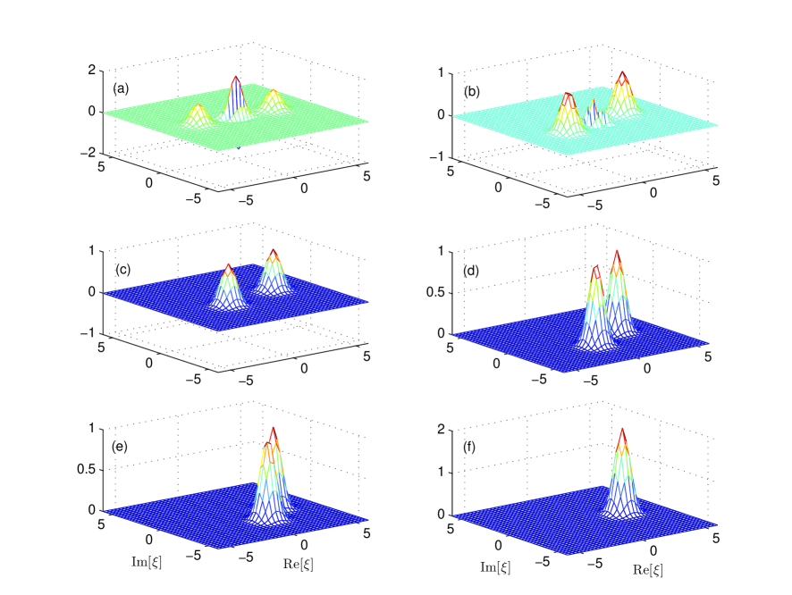
Figure 2: (Color online) Plot of the Wigner function $W(\xi)$ given in Eq. (32) for the state of the cantilever at different scaled times $\tau=\gamma t$: (a) $\tau=0$, (b) $\tau=0.06$, (c) $\tau=0.5$, (d) $\tau=0.1$, (e) $\tau=1.5$, (f) $\tau=20$. Other parameters are set as $\omega/\gamma=100$, $g/\gamma=-300$, $\beta=3$, and $\varphi=0$.

In Fig. 2, we plot the Wigner function given in Eq. (32) at different times for the case of $\varphi=0$ and $g_{s}=g$. When $t=0$, the Wigner function is right for the state $|\varphi_{+}\rangle$ given in Eq. (20) with $\beta=3$. This state is the so-called even Schrödinger cat state. We can see from Fig. 2(a) that there is some coherence in state (20). This is because the Wigner function in Fig. 2(a) exhibits some interference fringes (namely some oscillations), and these oscillations imply quantum coherence in the state. With the increase of the time $t$, we can find that the oscillations decrease gradually. At the same time, the positions of the two main peaks of the Wigner function rotate on the phase plain and move gradually to a point. This point corresponds approximately to the steady state of quantum master equation (22) for $T=0$. In fact, this steady state is a coherent state $|-ig_{s}/(\gamma/2+i\omega)\rangle\approx|2.999+0.015i\rangle$, which is obtained from Eq. (29) by taking the long time limit. Moreover, with the dissipative evolution, the negative values of the Wigner function will disappear gradually, which implies that the nonclassical properties of the cantilever decreases with the decoherence. Therefore, the actions of the environment and the driving force will destroy the coherence of the superposed coherent states and drive the cantilever into a steady coherent state.

IV Dynamical squeezing

In the above section, we have study the creation of superposed coherent states based on the obtained linear Hamiltonian. In this section, we study the creation of dynamical squeezing as an application of the nonlinear Hamiltonian. The created squeezed state not only exhibits nonclassical properties, but also is useful for precise measurement.

IV.1 Dynamical squeezing without dissipation

From Hamiltonian (11), we control the gate voltage $V_{g}$ such that $\omega_{0}=0$, then Hamiltonian (11) becomes

$$H=\omega a^{\dagger}a-\left[E_{J}+g^{\prime}(a^{\dagger}+a)^{2}\right]\sigma_{x}.$$ (34)

It can be seen from Hamiltonian (34) that if the qubit is initially prepared in one of the two eigenstates $|\pm\rangle$ of $\sigma_{x}$, then the qubit will stay in this state forever. Corresponding to the cases of the qubit in $|\pm\rangle$, the conditional Hamiltonians of the cantilever are

$$H_{k}=\omega_{k}a^{\dagger}a+g_{k}\left(a^{\dagger 2}+a^{2}\right),\hskip 14.22636ptk=\pm 1,$$ (35)

where $\omega_{k}=\omega+2g_{k}$ and $g_{k}=-k\times g^{\prime}$.

To diagonalize Hamiltonian (35), we introduce a unitary operator Wagner1986

$$\exp(-S_{k})=\exp\left[-\lambda_{k}\left(a^{2}-a^{{\dagger}2}\right)\right].$$ (36)

Using the commutative relations $[a,S_{k}]=-2\lambda_{k}a^{{\dagger}}$ and $[a^{{\dagger}},S_{k}]=-2\lambda_{k}a$, we obtain

$$e^{-S_{k}}ae^{S_{k}} =a\cosh(2\lambda_{k})-a^{{\dagger}}\sinh(2\lambda_{k}),$$ (37a)

$$e^{-S_{k}}a^{{\dagger}}e^{S_{k}} =a^{{\dagger}}\cosh(2\lambda_{k})-a\sinh(2\lambda_{k}).$$ (37b)

Application of the transform defined in Eq. (36) on Hamiltonian (35) leads to

$$\tilde{H}_{k} \equiv \exp(-S_{k})H_{k}\exp(S_{k})$$ (38)

$$= \Omega_{k}a^{{\dagger}}a+\Lambda_{k}\left(a^{{\dagger}2}+a^{2}\right)+C_{k},$$

where we introduce the following parameters

$$\Omega_{k} =\omega_{k}\cosh(4\lambda_{k})-2g_{k}\sinh(4\lambda_{k}),$$ (39a)

$$\Lambda_{k} =-\omega_{k}\sinh(4\lambda_{k})/2+g_{k}\cosh(4\lambda_{k}),$$ (39b)

$$C_{k} =\omega_{k}\sinh^{2}(2\lambda_{k})-g_{k}\sinh(4\lambda_{k}).$$ (39c)

By choosing proper parameter $\lambda_{k}$ to ensure $\Lambda_{k}=0$, namely $\tanh(4\lambda_{k})=2g_{k}/\omega_{k}$, then we may choose

$$\sinh(4\lambda_{k}) = \frac{2g_{k}}{\Omega_{k}},\hskip 14.22636pt\cosh(4\lambda_{k})=\frac{\omega_{k}}{\Omega_{k}},$$ (40)

where $\Omega_{k}=\sqrt{\omega_{k}^{2}-4g_{k}^{2}}$. Therefore we obtain the diagonalized Hamiltonian

$$\tilde{H}_{k}=\Omega_{k}a^{{\dagger}}a,\hskip 14.22636ptk=\pm 1.$$ (41)

The unitary evolution operator relating to Hamiltonian (41) is $V_{k}(t)=\exp(-i\tilde{H}_{k}t)$. Notice that in Eq. (41) we have discarded the constant term $C_{k}$.

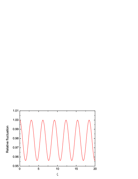
Figure 3: (Color online) Plot the relative fluctuation $(\Delta z)_{-1}^{2}/z_{0}^{2}$ given in Eq. (47) against the scaled evolution time $\zeta=\omega t$. Other parameter are set as $g^{\prime}/\omega=0.0115$. The relative fluctuation $(\Delta z)_{-1}^{2}/z_{0}^{2}<1$ means a squeezing of the position $z$ for the cantilever.

For investigation of the squeezing of the cantilever, we assume the cantilever is initially prepared in a coherent state $|\alpha\rangle$ and the qubit in states $|\pm\rangle$, where the coherent amplitude $\alpha$ is assumed to be a real number for simplicity. After a coherent evolution of a time $t$, the cantilever evolves into state

$$|\Phi_{k}(t)\rangle=e^{S_{k}}V_{k}(t)e^{-S_{k}}|\alpha\rangle.$$ (42)

Using the equation $a|\alpha\rangle=\alpha|\alpha\rangle$ and $|\alpha\rangle=e^{S_{k}}V^{\dagger}_{k}(t)e^{-S_{k}}|\Phi_{k}(t)\rangle$, we obtain

$$e^{S_{k}}V_{k}(t)e^{-S_{k}}ae^{S_{k}}V_{k}^{{\dagger}}(t)e^{-S_{k}}|\Phi_{k}(t)\rangle=\alpha|\Phi_{k}(t)\rangle,$$ (43)

which can be further written as

$$A_{k}(t)|\Phi_{k}(t)\rangle=\alpha|\Phi_{k}(t)\rangle,$$ (44)

with

$$A_{k}(t) \equiv e^{S_{k}}V_{k}(t)e^{-S_{k}}ae^{S_{k}}V_{k}^{{\dagger}}(t)e^{-S_{k}}$$ (45)

$$= [\cos(\Omega_{k}t)+i\cosh(4\lambda_{k})\sin(\Omega_{k}t)]a$$

$$+i\sinh(4\lambda_{k})\sin(\Omega_{k}t)a^{{\dagger}}.$$

The evolution of the cantilever follows the eigenstate of the quasi-excitation operator $A_{k}(t)$ with eigenvalue $\alpha$. According to Eq. (45), we can express the operators $a$ and $a^{{\dagger}}$ in terms of $A_{k}(t)$ and $A^{{\dagger}}_{k}(t)$,

$$a = [\cos\Omega_{k}t+i\cosh(4\lambda_{k})\sin(\Omega_{k}t)]A_{k}(t)$$ (46)

$$+i\sinh(4\lambda_{k})\sin(\Omega_{k}t)A^{{\dagger}}_{k}(t).$$

Based on Eq. (46), the fluctuation $(\Delta z)_{k}^{2}=\langle z^{2}\rangle_{k}-\langle z\rangle_{k}^{2}$ of the coordinator $z$ for the cantilever is obtained as

$$(\Delta z)_{k}^{2}(t) = z_{0}^{2}\left[\cosh(4\lambda_{k})-\sinh(4\lambda_{k})\right]^{2}\sin^{2}(\Omega_{k}t)$$ (47)

$$+\cos^{2}(\Omega_{k}t).$$

From Eq. (47), we find that, only in the case of $k=-1$, the squeezing of the position $z$ of the cantilever occurs. In Fig. 3, we plot the relative fluctuation $(\Delta z)_{-1}^{2}/z_{0}^{2}$ as a function of the scaled evolution time $\zeta=\omega t$. Figure 3 shows a periodic squeezing with the scaled evolution time $\zeta$.

IV.2 Dynamical squeezing with dissipation

In the above subsection, we study the dynamical squeezing for the ideal case in which there is no dissipation. However, any systems will couple inevitably with the environment. In this subsection, we consider the dynamical squeezing of the cantilever by taking the environment into account. In the presence of an environment, the evolution of the cantilever is governed by the following quantum master equation

$$\dot{\rho}=i\left[\rho\left(t\right),H_{k}\right]+\mathcal{L}\rho\left(t\right),$$ (48)

where the Hamiltonian $H_{k}$ has been given in Eq. (35), and the superoperator has been given in Eq. (23). Based on quantum master equation (48), we can obtain the following equations of motion,

$$\frac{d}{dt}\langle a\rangle =-i\omega_{k}\langle a\rangle-2ig_{k}\langle a^{\dagger}\rangle-\frac{\gamma}{2}\langle a\rangle,$$ (49a)

$$\frac{d}{dt}\langle a^{\dagger}\rangle =i\omega_{k}\langle a^{\dagger}\rangle+2ig_{k}\langle a\rangle-\frac{\gamma}{2}\langle a^{\dagger}\rangle,$$ (49b)

$$\frac{d}{dt}\langle a^{2}\rangle =-(\gamma+2i\omega_{k})\langle a^{2}\rangle-4ig_{k}\langle a^{\dagger}a\rangle-2ig_{k},$$ (49c)

$$\frac{d}{dt}\langle a^{\dagger 2}\rangle =-(\gamma-2i\omega_{k})\langle a^{\dagger 2}\rangle+4ig_{k}\langle a^{\dagger}a\rangle+2ig_{k},$$ (49d)

$$\frac{d}{dt}\langle a^{\dagger}a\rangle =-\gamma\langle a^{\dagger}a\rangle-2ig_{k}\langle a^{\dagger 2}\rangle+2ig_{k}\langle a^{2}\rangle+\gamma\bar{n}_{th}.$$ (49e)

According to the definition of $z=z_{0}(a+a^{\dagger})$, the relative fluctuation of the coordinator operator $z$ can be written as

$$\frac{(\Delta z(t))_{k}^{2}}{z_{0}^{2}} = \left(\langle a^{2}\rangle-\langle a\rangle^{2}+\langle a^{\dagger 2}\rangle-\langle a^{\dagger}\rangle^{2}\right.$$ (50)

$$\left.+2\langle a^{\dagger}a\rangle-2\langle a^{\dagger}\rangle\langle a\rangle+1\right).$$

Therefore, under a given initial condition, we can obtain the solutions of Eq. (49), and then the evolution of the fluctuation $(\Delta z)^{2}(t)$ can be obtained. In the following we suppose the cantilever is initially prepared in a vacuum state $|0\rangle$.

In principle, the solutions of Eq. (49) can be obtained. However, we do not present the solutions here since there are very complicate. In Fig. 4, we plot the relative fluctuation $(\Delta z)_{-1}^{2}(t)/z_{0}^{2}$ against the time $t$ for different temperatures.

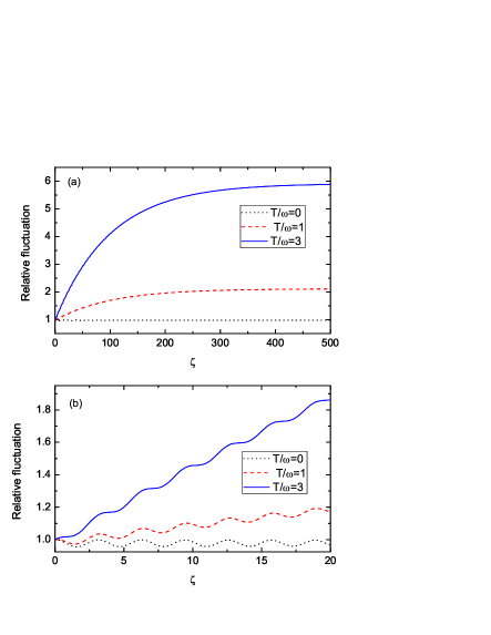
Figure 4: (Color online) (a) Plot of the relative fluctuation $(\Delta z)_{-1}^{2}/z_{0}^{2}$ given in Eq. (52) vs the scaled evolution time $\zeta=\omega t$ for different temperatures: $T/\omega=0$ (dotted line), $T/\omega=1$ (dashed line), $T/\omega=3$ (solid line). (b) Amplificatory plot of figure (a) from $\zeta=0$ to $20$. Other parameters are set as $\gamma/\omega=0.01$, and $g^{\prime}/\omega=0.0115$.

It can be seen from Fig. 4 that the relative fluctuation $(\Delta z)_{-1}^{2}/z_{0}^{2}$ evolves gradually approaching a steady-state value with the increase of the time $t$. For a short time, the relative fluctuation evolves with some oscillations. At the same time, the relative fluctuation increases with the increase of the bath temperature $T$. Therefore, we can obtain a conclusion that the high temperature $T$ can destroy the squeezing for the position $z$ of the cantilever.

For obtaining the steady-state properties of the squeezing, we obtain the steady-state solution of Eq. (49) as

$$\langle a(\infty)\rangle =\langle a^{\dagger}(\infty)\rangle=0,$$ (51a)

$$\langle a^{2}(\infty)\rangle =-\frac{2g_{k}(2\bar{n}_{th}+1)(2\omega_{k}+i\gamma)}{\gamma^{2}+4\omega_{k}^{2}-16g_{k}^{2}},$$ (51b)

$$\langle a^{\dagger 2}(\infty)\rangle =-\frac{2g_{k}(2\bar{n}_{th}+1)(2\omega_{k}-i\gamma)}{\gamma^{2}+4\omega_{k}^{2}-16g_{k}^{2}},$$ (51c)

$$\langle a^{\dagger}a(\infty)\rangle =\bar{n}_{th}+\frac{8g_{k}^{2}(2\bar{n}_{th}+1)}{\gamma^{2}+4\omega_{k}^{2}-16g_{k}^{2}}.$$ (51d)

Then the steady-state fluctuation is

$$\frac{(\Delta z(\infty))_{k}^{2}}{z_{0}^{2}} = \frac{(2\bar{n}_{th}+1)[\gamma^{2}+4\omega_{k}(\omega_{k}-2g_{k})]}{\gamma^{2}+4\omega_{k}^{2}-16g_{k}^{2}}.$$ (52)

In Fig. 5, we plot the steady-state relative fluctuation $(\Delta z(\infty))_{-1}^{2}/z_{0}^{2}$ as a function of the temperature $T$. It can be seen from Fig. 5 that the steady-state relative fluctuation increases with the increase of the temperature $T$. We can see a transition from squeezing to nonsqueezing when the temperature across a critical temperature $T_{\textrm{c}}$, which can be obtained from Eq. (52) for the case of $k=-1$,

$$\frac{T_{\textrm{c}}}{\omega}=\frac{1}{\ln\left(\frac{\gamma^{2}}{4\omega g^{\prime}}+\frac{\omega}{g^{\prime}}+3\right)}.$$ (53)

According to the parameters, we calculate the critical temperature in Fig. 5 is $T_{\textrm{c}}/\omega=0.222$.

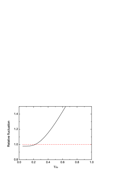
Figure 5: (Color online) Plot of the steady-state relative fluctuation $(\Delta z(\infty))_{-1}^{2}/z_{0}^{2}$ against the scaled temperature $T/\omega$. Other parameters are set as those in Fig. 4. Figure shows a transition from squeezing to nonsqueezing with the increase of the temperature of the environment.

V Discussions and conclusions

We note that the two types of subsystems in our scheme, the superconducting charge qubit and the cantilever, have been well prepared in current experiments. Hence, it is possible to experimentally realize the scheme proposed in this paper within the reach of present-day techniques. Here we give a possible estimation of coupled-system parameters based on these published experimental parameters of the charge qubit and the cantilevers. The most important parameters in our model are the two coupling strengths $g$ and $g^{\prime}$ given in Eqs. (12) and (34), respectively. According to the current experimental conditions Sidles1995 ; Mamin2007 , we take the following parameters. As an example, we choose a cantilever with a fundamental frequency $\omega\approx 2\pi\times 2$ MHz, $\gamma=2\pi\times 20$ kHz, and $z_{0}\approx 5\times 10^{-13}$ m. A magnetic tip produces a magnetic gradient of $|\partial B_{z}/\partial z|\approx 10^{-7}$ T/m at an approximate distance $50$ nm above the superconducting loop. Then we obtian $C=|\partial B_{z}/\partial z|z_{0}\approx 5\times 10^{-6}$ T. We choose the area of the superconducting loop $S\approx 10^{-12}$ m², and $E_{J}\approx 5$ GHz. Then we get $\phi\approx 2.4\pi\times 10^{-3}$, which is suitable for making the approximations of expanding the sine and cosine functions up to the first and second orders, respectively. Accordingly, the coupling strengths $g\approx-2\pi\times 6$ MHz and $g^{\prime}\approx 2\pi\times 23$ kHz. Notice that the figures in the above sections are plotted in terms of these parameters.

In conclusion, we have designed a theoretical scheme to realize tailorable couplings between a cantilever and a superconducting charge qubit. By choosing proper parameters, both linear and nonlinear couplings can be achieved. We have also shown how to generate superposed coherent states and dynamical squeezing in the cantilever based on the obtained couplings. We have investgated the influence of the environment on quantum states of the cantilever. It has been indicated that decoherence induced by the environment can drive the cantilever from superposed coherent states into the steady coherent state. When the cantilever is initially in a coherent state, we have shown that there exists periodic position squeezing for the cantilever. Especially, it is found that under the action of the environment the cantilever can evolve from the vacuum state to a steady state with position squeezing under a critical temperature of the environment. Therefore, the environment can induce the steady-state position squeezing of the cantilever. This reveals a new mechanism to create the steady-state squeezing and sheds new light on production of nonclassical effects of the cantilever. Finally, it should be emphasized that the experimental realization of the scheme proposed in the present paper deserves further investigation.

Appendix A Derivation of quantum master equation (26)

In this Appendix, we give a detailed derivation of the transform from quantum master equation (22) to equation (26). Starting from the quantum master equation

$$\dot{\rho} = i[\rho,\omega a^{\dagger}a+g_{s}(a^{\dagger}+a)]$$ (54)

$$+\frac{\gamma}{2}(\bar{n}+1)(2a\rho a^{\dagger}-a^{\dagger}a\rho-\rho a^{\dagger}a)$$

$$+\frac{\gamma}{2}\bar{n}(2a^{\dagger}\rho a-aa^{\dagger}\rho-\rho aa^{\dagger}),$$

we first make a rotation transform,

$$\rho^{\left(1\right)}=R^{\dagger}\left(\theta\right)\rho R\left(\theta\right),\hskip 14.22636ptR\left(\theta\right)=e^{-i\theta a^{\dagger}a},$$ (55)

then we obtain $\rho=R\left(\theta\right)\rho^{\left(1\right)}R^{\dagger}\left(\theta\right)$ and

$$\dot{\rho} = -i\dot{\theta}a^{\dagger}aR\left(\theta\right)\rho^{\left(1\right)}R^{\dagger}\left(\theta\right)+R\left(\theta\right)\dot{\rho}^{\left(1\right)}R^{\dagger}\left(\theta\right)$$ (56)

$$+i\dot{\theta}R\left(\theta\right)\rho^{\left(1\right)}a^{\dagger}aR^{\dagger}\left(\theta\right).$$

Substitution of Eq. (56) into quantum master equation (54) leads to

$$\dot{\rho}^{\left(1\right)} = i(\omega-\dot{\theta})\rho^{\left(1\right)}a^{\dagger}a-i(\omega-\dot{\theta})a^{\dagger}a\rho^{\left(1\right)}$$ (57)

$$+ig_{s}\rho^{\left(1\right)}\left(a^{\dagger}e^{i\theta}+ae^{-i\theta}\right)-ig_{s}\left(a^{\dagger}e^{i\theta}+ae^{-i\theta}\right)\rho^{\left(1\right)}$$

$$+\frac{\gamma}{2}\left(\bar{n}+1\right)\left(2a\rho^{(1)}a^{\dagger}-a^{\dagger}a\rho^{(1)}-\rho^{(1)}a^{\dagger}a\right)$$

$$+\frac{\gamma}{2}\bar{n}\left(2a^{\dagger}\rho^{(1)}a-aa^{\dagger}\rho^{(1)}-\rho^{(1)}aa^{\dagger}\right),$$

where we have used the relations

$$\left[R\left(\theta\right),a^{\dagger}a\right] =\left[R^{\dagger}\left(\theta\right),a^{\dagger}a\right]=0,$$ (58a)

$$R^{\dagger}\left(\theta\right)a^{\dagger}R\left(\theta\right) =e^{i\theta a^{\dagger}a}a^{\dagger}e^{-i\theta a^{\dagger}a}=a^{\dagger}e^{i\theta},$$ (58b)

$$R^{\dagger}\left(\theta\right)aR\left(\theta\right) =e^{i\theta a^{\dagger}a}ae^{-i\theta a^{\dagger}a}=ae^{-i\theta}.$$ (58c)

We choose a proper $\theta$ to ensure $\omega-\dot{\theta}=0$. Under the initial condition $\theta(0)=0$, we get

$$\theta(t)=\omega t.$$ (59)

Then we obtain

$$\dot{\rho}^{(1)} = ig_{s}\left[\rho^{(1)},a^{\dagger}e^{i\omega t}+ae^{-i\omega t}\right]$$ (60)

$$+\frac{\gamma}{2}(\bar{n}+1)\left(2a\rho^{(1)}a^{\dagger}-a^{\dagger}a\rho^{(1)}-\rho^{(1)}a^{\dagger}a\right)$$

$$+\frac{\gamma}{2}\bar{n}\left(2a^{\dagger}\rho^{(1)}a-aa^{\dagger}\rho^{(1)}-\rho^{(1)}aa^{\dagger}\right).$$

Since the first term at the right-hand side of Eq. (60) is a driving term, in the following, we make a displacement transform

$$\rho^{\left(2\right)} = D^{\dagger}\left(\alpha\right)\rho^{\left(1\right)}D\left(\alpha\right),\hskip 14.22636ptD\left(\alpha\right)=e^{\alpha a^{\dagger}-\alpha^{\ast}a},$$ (61)

then we obtain $\rho^{\left(1\right)}=D\left(\alpha\right)\rho^{\left(2\right)}D^{\dagger}\left(\alpha\right)$ and

$$\dot{\rho}^{\left(1\right)} = \dot{D}\left(\alpha\right)\rho^{\left(2\right)}D^{\dagger}\left(\alpha\right)+D\left(\alpha\right)\dot{\rho}^{\left(2\right)}D^{\dagger}\left(\alpha\right)$$ (62)

$$+D\left(\alpha\right)\rho^{\left(2\right)}\left(t\right)\dot{D}^{\dagger}\left(\alpha\right).$$

Here we need to calculate the expressions for $\dot{D}\left(\alpha\right)$ and $\dot{D}^{\dagger}\left(\alpha\right)$. Making use of $D\left(\alpha\right)=e^{-\frac{\left|\alpha\right|^{2}}{2}}e^{\alpha a^{\dagger}}e^{-\alpha^{\ast}a}$, we have

$$\dot{D}\left(\alpha\right) = \frac{d}{dt}\left(e^{-\frac{\left|\alpha\right|^{2}}{2}}\right)e^{\alpha a^{\dagger}}e^{-\alpha^{\ast}a}+e^{-\frac{\left|\alpha\right|^{2}}{2}}\frac{d}{dt}\left(e^{\alpha a^{\dagger}}\right)e^{-\alpha^{\ast}a}$$

$$+e^{-\frac{\left|\alpha\right|^{2}}{2}}e^{\alpha a^{\dagger}}\frac{d}{dt}\left(e^{-\alpha^{\ast}a}\right)$$

$$= -\frac{1}{2}(\dot{\alpha}\alpha^{\ast}+\alpha\dot{\alpha}^{\ast})D(\alpha)+\dot{\alpha}D(\alpha)e^{\alpha^{\ast}a}a^{\dagger}e^{-\alpha^{\ast}a}$$

$$-\dot{\alpha}^{\ast}D(\alpha)a$$

$$= -\frac{1}{2}\left(\alpha\dot{\alpha}^{\ast}-\dot{\alpha}\alpha^{\ast}\right)D(\alpha)+D(\alpha)(\dot{\alpha}a^{\dagger}-\dot{\alpha}^{\ast}a),$$

where we have used the formula $e^{\alpha^{\ast}a}a^{\dagger}e^{-\alpha^{\ast}a}=a^{\dagger}+\alpha^{\ast}$. Similarly, we obtain

$$\dot{D}^{\dagger}(\alpha) = -\frac{1}{2}(\dot{\alpha}\alpha^{\ast}-\alpha\dot{\alpha}^{\ast})D^{\dagger}(\alpha)+(\dot{\alpha}^{\ast}a-\dot{\alpha}a^{\dagger})D^{\dagger}(\alpha).$$

Substitution of Eqs. (62), (A), and (A) into Eq. (60), we obtain

$$\dot{\rho}^{(2)} = \frac{\gamma}{2}(\bar{n}+1)\left(2a\rho^{(2)}a^{\dagger}-a^{\dagger}a\rho^{(2)}-\rho^{(2)}a^{\dagger}a\right)$$ (65)

$$+\frac{\gamma}{2}\bar{n}\left(2a^{\dagger}\rho^{(2)}a-aa^{\dagger}\rho^{(2)}-\rho^{(2)}aa^{\dagger}\right)$$

$$+\left(\dot{\alpha}^{\ast}-ig_{s}e^{-i\omega t}+\frac{\gamma}{2}\alpha^{\ast}\right)\left(a\rho^{(2)}(t)-\rho_{s}^{(2)}a\right)$$

$$-\left(\dot{\alpha}+ig_{s}e^{i\omega t}+\frac{\gamma}{2}\alpha\right)\left(a^{\dagger}\rho^{(2)}-\rho^{(2)}a^{\dagger}\right).$$

Therefore, if we choose a proper $\alpha$ such that

$$\dot{\alpha}+ig_{s}e^{i\omega t}+\frac{\gamma}{2}\alpha = 0,$$ (66)

then we obtain the quantum master equation (26). The solution of Eq. (66) can be obtained as

$$\alpha(t) = \frac{ig_{s}}{\frac{\gamma}{2}+i\omega}\left(e^{-\frac{\gamma t}{2}}-e^{i\omega t}\right)$$ (67)

under the initial condition $\alpha(0)=0$.

Appendix B Derivation of Eq. (29)

In this Appendix, we derive in detail the evolution of the cantilever governed by quantum master equation (22). For an initial state $\rho(0)$, the state of the cantilever at time $t$ can be obtained through the processes $\rho(0)\rightarrow\rho^{(2)}(0)\rightarrow\rho^{(2)}(t)\rightarrow\rho(t)$. The relationship between states $\rho(0)$ and $\rho^{(2)}(0)$ is

$$\rho^{(2)}(0) = D^{\dagger}(\alpha(0))R^{\dagger}(\theta(0))\rho(0)R(\theta(0))D(\alpha(0))$$ (68)

$$= \rho(0).$$

For the initial state

$$|\psi(0)\rangle=\mathcal{N}_{\varphi}(|\beta\rangle+e^{i\varphi}|-\beta\rangle),$$ (69)

we have

$$\rho^{(2)}(0) = \mathcal{N}_{\varphi}^{2}(|\beta\rangle+e^{i\varphi}|-\beta\rangle)(\langle\beta|+e^{-i\varphi}\langle-\beta|).$$ (70)

The evolution process from state $\rho^{\left(2\right)}\left(0\right)$ to $\rho^{\left(2\right)}\left(t\right)$ is governed by the quantum master equation

$$\dot{\rho}^{(2)}(t) = \frac{\gamma}{2}(\bar{n}+1)\left(2a\rho^{\left(2\right)}(t)a^{\dagger}-a^{\dagger}a\rho^{(2)}(t)-\rho^{(2)}(t)a^{\dagger}a\right)$$ (71)

$$+\frac{\gamma}{2}\bar{n}\left(2a^{\dagger}\rho^{\left(2\right)}a-aa^{\dagger}\rho^{\left(2\right)}\left(t\right)-\rho^{\left(2\right)}(t)aa^{\dagger}\right).$$

In principle, the above master equation can be solved by the superoperator method Burnett . However, for simplicity, we only consider the zero temperature case in the following. At zero temperature, the master equation reduces to

$$\dot{\rho}^{(2)} = \frac{\gamma}{2}\left(2a\rho^{(2)}(t)a^{\dagger}-a^{\dagger}a\rho^{(2)}(t)-\rho^{(2)}(t)a^{\dagger}a\right).$$ (72)

Denoting the two superoperators

$$J\rho^{(2)}(t) =a\rho^{(2)}(t)a^{\dagger},$$ (73a)

$$L\rho^{(2)}(t) =-\frac{1}{2}\left(a^{\dagger}a\rho^{(2)}(t)+\rho^{(2)}(t)a^{\dagger}a\right),$$ (73b)

then the map from initial state $\rho^{(2)}(0)$ to $\rho^{(2)}(t)$ at time $t$ is determined by

$$\rho^{(2)}(t)=\exp(\gamma tL)\exp[(1-\exp(-\gamma t))J]\rho^{(2)}(0).$$ (74)

According to the initial state given in Eq. (70), we have

$$\rho^{\left(2\right)}\left(t\right) = \mathcal{N}_{\varphi}^{2}\left(\left|\beta e^{-\frac{\gamma t}{2}}\right\rangle\left\langle\beta e^{-\frac{\gamma t}{2}}\right|+e^{-i\varphi}e^{\Delta_{r}}\left|\beta e^{-\frac{\gamma t}{2}}\right\rangle\left\langle-\beta e^{-\frac{\gamma t}{2}}\right|\right.$$

$$\left.+e^{i\varphi}e^{\Delta_{r}}\left|-\beta e^{-\frac{\gamma t}{2}}\right\rangle\left\langle\beta e^{-\frac{\gamma t}{2}}\right|+\left|-\beta e^{-\frac{\gamma t}{2}}\right\rangle\left\langle-\beta e^{-\frac{\gamma t}{2}}\right|\right),$$

where we introduce the parameter $\Delta_{r}=2|\beta|^{2}(e^{-\gamma t}-1)$. During the derivation of the above equation (LABEL:B10), we have used the formulas

$$\exp[xJ]|r\rangle\langle s| =\exp[xrs^{\ast}]|r\rangle\langle s|,$$ (76a)

$$\exp(\gamma tL)|r\rangle\langle s| =\exp[-(|r|^{2}+|s|^{2})(1-e^{-\gamma t})/2]$$

$$\times\left|re^{-\frac{\gamma t}{2}}\right\rangle\left\langle se^{-\frac{\gamma t}{2}}\right|,$$ (76b)

for coherent states $|r\rangle$ and $|s\rangle$.

For obtaining the state in the Schrödinger picture at time $t$, we use the relation $\rho^{(1)}(t)=D(\alpha(t))\rho^{(2)}(t)D^{\dagger}(\alpha(t))$ to obtain

$$D\left(\alpha\left(t\right)\right)\rho^{\left(2\right)}\left(t\right)D^{\dagger}\left(\alpha\left(t\right)\right)$$

$$= \mathcal{N}_{\varphi}^{2}\left(\left|\alpha\left(t\right)+\beta e^{-\frac{\gamma t}{2}}\right\rangle\left\langle\alpha\left(t\right)+\beta e^{-\frac{\gamma t}{2}}\right|\right.$$ (77)

$$\left.+\left|\alpha\left(t\right)-\beta e^{-\frac{\gamma t}{2}}\right\rangle\left\langle\alpha\left(t\right)-\beta e^{-\frac{\gamma t}{2}}\right|\right.$$

$$\left.+e^{-i\varphi}e^{\Delta_{r}+i\Delta_{i}}\left|\alpha\left(t\right)+\beta e^{-\frac{\gamma t}{2}}\right\rangle\left\langle\alpha\left(t\right)-\beta e^{-\frac{\gamma t}{2}}\right|\right.$$

$$\left.+e^{i\varphi}e^{\Delta_{r}-i\Delta_{i}}\left|\alpha\left(t\right)-\beta e^{-\frac{\gamma t}{2}}\right\rangle\left\langle\alpha\left(t\right)+\beta e^{-\frac{\gamma t}{2}}\right|\right)$$

where we introduce the parameter $\Delta_{i}=2\textrm{Im}(\alpha(t)\beta^{\ast}\exp(-\gamma t/2))$. Here we have used the formula

$$D(\alpha)|\beta\rangle=e^{i\textrm{Im}(\alpha\beta^{\ast})}|\alpha+\beta\rangle$$ (78)

for coherent state $|\beta\rangle$. And then we use the relation $\rho(t)=R(\theta)\rho^{(1)}(t)R^{\dagger}(\theta)$ to obtain the state

$$\rho\left(t\right) = \mathcal{N}_{\varphi}^{2}\left(\left|\beta_{+}\right\rangle\left\langle\beta_{+}\right|+e^{-i\varphi}e^{\Delta_{r}+i\Delta_{i}}\left|\beta_{+}\right\rangle\left\langle\beta_{-}\right|\right.$$ (79)

$$\left.+e^{i\varphi}e^{\Delta_{r}-i\Delta_{i}}\left|\beta_{-}\right\rangle\left\langle\beta_{+}\right|+\left|\beta_{-}\right\rangle\left\langle\beta_{-}\right|\right),$$

where we introduce the following two parameters

$$\beta_{\pm}=\left(\alpha(t)\pm\beta e^{-\frac{\gamma t}{2}}\right)e^{-i\omega t}.$$ (80)

References

- (1) J. A. Sidles, J. L. Garbinni, K. J. Bruland, D. Rugar, O. Züger, S. Hoen, and C. S. Yannoni, Rev. Mod. Phys. 67, 249 (1995).
- (2) H. J. Mamin, R. Budakian, B. W. Chui, and D. Rugar, Phys. Rev. Lett. 91, 207604 (2003); D. Rugar, R. Budakian, H. J. Mamin, and B. W. Chui, Nature (London) 430, 329 (2004).
- (3) G. P. Berman, F. Borgonovi, V. N. Gorshkov, and V. I. Tsifrinovich, Magnetic Resonance Force Microscopy and a Single-Spin Measurement (World Scientific, Singapore, 2006).
- (4) A. N. Cleland, Foundations of Nanomechanics: From Solid-State Theory to Device Applications (Springer, Berlin, 2003).
- (5) M. P. Blencowe, Phys. Rep. 395, 159 (2004).
- (6) K. C. Schwab and M. L. Roukes, Phys. Today 58, 36 (2005).
- (7) D. P. DiVincenzo, Phys. Rev. A 51, 1015 (1995).
- (8) G. P. Berman, G. D. Doolen, P. C. Hammel, and V. I. Tsifrinovich, Phys. Rev. B 61, 14694 (2000).
- (9) M. LaHaye, O. Buu, B. Camarota, and K. Schwab, Science 304, 74 (2004).
- (10) W. H. Zurek, Phys. Today 44(10), 36 (1991).
- (11) I. Katz, A. Retzker, R. Straub, and R. Lifshitz, Phys. Rev. Lett. 99, 040404 (2007).
- (12) A. D. Armour, M. P. Blencowe, and K. C. Schwab, Phys. Rev. Lett. 88, 148301 (2002).
- (13) W. Marshall, C. Simon, R. Penrose, and D. Bouwmeester, Phys. Rev. Lett. 91, 130401 (2003).
- (14) X. M. H. Huang, C. A. Zorman, M. Mehregany, and M. L. Roukes, Nature (London) 421, 496 (2003).
- (15) R. G. Knobel and A. N. Cleland, Nature (London) 424, 291 (2003).
- (16) A. Gaidarzhy, G. Zolfagharkhani, R. L. Badzey, and P. Mohanty, Phys. Rev. Lett. 94, 030402 (2005).
- (17) I. Wilson-Rae, P. Zoller, and A. Imamoglu, Phys. Rev. Lett. 92, 075507 (2004).
- (18) C. H. Metzger and K. Karrai, Nature (London) 432, 1002 (2004).
- (19) P. Zhang, Y. D. Wang, and C. P. Sun, Phys. Rev. Lett. 95, 097204 (2005).
- (20) A. Naik, O. Buu, M. D. LaHaye, A. D. Armour, A. A. Clerk, M. P. Blencowe, and K. C. Schwab, Nature (London) 443, 193 (2006).
- (21) S. Gigan, H. R. Böhm, M. Paternostro, F. Blaser, G. Langer, J. B. Hertzberg, K. C. Schwab, D. Bäuerle, M. Aspelmeyer, and A. Zeilinger, Nature (London) 444, 67 (2006).
- (22) O. Arcizet, P. F. Cohadon, T. Briant, M. Pinard, and A. Heidmann, Nature (London) 444, 71 (2006).
- (23) D. Kleckner and D. Bouwmeester, Nature (London) 444, 75 (2006).
- (24) M. Poggio, C. L. Degen, H. J. Mamin, and D. Rugar, Phys. Rev. Lett. 99, 017201 (2007).
- (25) I. Wilson-Rae, N. Nooshi, W. Zwerger, and T. J. Kippenberg, Phys. Rev. Lett. 99, 093901 (2007);
- (26) F. Marquardt, J. P. Chen, A. A. Clerk, and S. M. Girvin, Phys. Rev. Lett. 99, 093902 (2007).
- (27) F. Xue, Y. D. Wang, Y. X. Liu, and F. Nori, Phys. Rev. B 76, 205302 (2007).
- (28) Y. Li, Y. D. Wang, F. Xue, and C. Bruder, Phys. Rev. B 78, 134301 (2008).
- (29) Y. D. Wang, Y. Li, F. Xue, C. Bruder, and K. Semba, Phys. Rev. B 80, 144508 (2009).
- (30) S. H. Ouyang, J. Q. You, and F. Nori, Phys. Rev. B 79, 075304 (2009).
- (31) L. F. Wei, Y. X. Liu, C. P. Sun, and F. Nori, Phys. Rev. Lett. 97, 237201 (2006); Y. B. Gao, S. Yang, Y. X. Liu, C. P. Sun, and F. Nori, arXiv:0902.2512; Y. X. Liu, A. Miranowicz, Y. B. Gao, C. P. Sun, and F. Nori, arXiv:0910.3066.
- (32) F. Xue, Y. X. Liu, C. P. Sun, and F. Nori, Phys. Rev. B 76, 064305 (2007).
- (33) J. Q. Liao and L. M. Kuang, Eur. Phys. J. B 63, 79 (2008).
- (34) K. Jacobs, P. Lougovski, and M. Blencowe, Phys. Rev. Lett. 98, 147201 (2007).
- (35) J. Siewert, T. Brandes, and G. Falci, Phys. Rev. B 79, 024504 (2009).
- (36) L. Tian, Phys. Rev. B 72, 195411 (2005).
- (37) P. Rabl, A. Shnirman, and P. Zoller, Phys. Rev. B 70, 205304 (2004).
- (38) R. Ruskov, K. Schwab, and A. N. Korotkov, Phys. Rev. B 71, 235407 (2005).
- (39) X. X. Zhou and A. Mizel, Phys. Rev. Lett. 97, 267201 (2006).
- (40) J. Zhang, Y. X. Liu, and Franco Nori, Phys. Rev. A 79, 052102 (2009).
- (41) W. Y. Huo and G. L. Long. Appl. Phys. Lett. 92, 133102 (2008).
- (42) R. Almog, S. Zaitsev, O. Shtempluck, and E. Buks, Phys. Rev. Lett. 98, 078103 (2007).
- (43) J. Eisert, M. B. Plenio, S. Bose, and J. Hartley, Phys. Rev. Lett. 93, 190402 (2004).
- (44) S. Bose and G. S. Agarwal, New J. Phys. 8, 34 (2005).
- (45) D. Vitali, P. Tombesi, M. J. Woolley, A. C. Doherty, and G. J. Milburn, Phys. Rev. A 76, 042336 (2007).
- (46) M. O. Scully and M. S. Zubairy, Quantum Optics (Cambridge Univ. Press, Cambridge, 1997).
- (47) E. K. Irish, J. Gea-Banacloche, I. Martin, and K. C. Schwab, Phys. Rev. B 72, 195410 (2005).
- (48) C. P. Sun, L. F. Wei, Y. X. Liu, and F. Nori, Phys. Rev. A 73, 022318 (2006).
- (49) F. Xue, Y. D. Wang, C. P. Sun, H. Okamoto, H. Yamaguchi, and K. Semba, New J. Phys. 9, 35 (2007).
- (50) M. D. LaHaye, J. Suh, P. M. Echternach, K. C. Schwab, and M. L. Roukes, Nature (London) 459, 960 (2009).
- (51) M. P. Blencowe and E. Buks, Phys. Rev. B 76, 014511 (2007).
- (52) T. Rocheleau, T. Ndukum, C. Macklin, J. B. Hertzberg, A. A. Clerk, and K. C. Schwab, Nature 463, 72 (2009).
- (53) J. B. Hertzberg, T. Roucheleau, T. Ndukum, M. Savva, A. A. Clerk, and K. C. Schwab, Nature Physics 6, 213 (2009).
- (54) L. Tian and P. Zoller, Phys. Rev. Lett. 93, 266403 (2004).
- (55) P. Treutlein, D. Hunger, S. Camerer, T. W. Hänsch, and J. Reichel, Phys. Rev. Lett. 99, 140403 (2007).
- (56) D. Hunger, S. Camerer, T. W. Hänsch, D. Kö nig, J. Kotthaus, J. Reichel, and P. Treutlein, Phys. Rev. Lett. 104, 143002 (2010).
- (57) R. Kanamoto and P. Meystre, Phys. Rev. Lett. 104, 063601 (2010).
- (58) N. Lambert, I. Mahboob, M. Pioro-Ladrière, Y. Tokura, S. Tarucha, and H. Yamaguchi, Phys. Rev. Lett. 100, 136802 (2008).
- (59) N. Lambert and F. Nori, Phys. Rev. B 78, 214302 (2008).
- (60) S. D. Bennett, L. Cockins, Y. Miyahara, P. Gr tter, and A. A. Clerk, Phys. Rev. Lett. 104, 017203 (2010); L. Cockinsa, Y. Miyaharaa, S. D. Bennetta, A. A. Clerka, S. Studenikinb, P. Pooleb, A. Sachrajdab, and P. Gruttera, Proceedings of the National Academy of Sciences 107, 9496 (2010)
- (61) K. Jacobs, Phys. Rev. Lett. 99, 117203 (2007).
- (62) Y. Makhlin, G. Schön, and A. Shnirman, Rev. Mod. Phys. 73, 357 (2001).
- (63) J. Q. You and F. Nori, Phys. Today 58(11), 42 (2005).
- (64) Y. Nakamura, Y. A. Pashkin, and J. S. Tsai, Nature (London) 398, 786 (1999).
- (65) Y. Makhlin, G. Schoen, and A. Shnirman, Nature (London) 398, 305 (1999).
- (66) F. Xue, L. Zhong, Y. Li, and C. P. Sun, Phys. Rev. B 75, 033407 (2007).
- (67) P. C. Haljan, K. A. Brickman, L. Deslauriers, P. J. Lee, and C. Monroe, Phys. Rev. Lett. 94, 153602 (2005).
- (68) J. Q. Liao and L. M. Kuang, J. Phys. B 40, 1845 (2007).
- (69) C. C. Gerry and P. L. Knight, Introductory Quantum Optics (Cambridge University Press, Cambridge, 2004).
- (70) S. M. Burnett and P. M. Radmore, Methods in Theoretical Quantum Optics (Clarendon press, Oxford, 1997).
- (71) M. Wagner, Unitary Transformations in Solid State Physics (Elsevier, Amsterdam, 1986).
- (72) H. J. Mamin, M. Poggio, C. L. Degen, and D. Rugar, Nat. Nanotechnol. 2, 301 (2007).