Constraints on conductances for Y-junction of quantum wires

Abstract

We consider the Y-junction, connecting three quantum wires, in the scattering states formalism. In the absence of fermionic interaction we analyze the restrictions on the values of conductance matrix, imposed by the unitarity of scattering $S$-matrix. Using the combination of numerical and analytical results, we describe the four-dimensional body of values of reduced conductance matrix. We show that this body touches the unit sphere at six points only, in accordance with Birkhoff-von Neumann theorem. It implies that the Abelian bosonization analysis for the vanishing interaction strength can be performed only in the vicinity of these six points.

I Introduction and model

Investigation of the properties of electronic systems in reduced dimensionality is the subject of ongoing active studies, both theoretical and experimental. The effects of electronic interaction play a major role in one spatial dimension and lead to a formation of the Luttinger liquid state Giamarchi (2003). The idealized Luttinger liquid is best described in terms of its excitations within the bosonization approach. The imperfections in quantum wires, such as impurities, are thoroughly investigated by different methods, see Aristov and Wölfle (2009) and references therein. In view of potential technological applications, it is also desirable to theoretically analyze junctions of several quantum wires. Such analysis for the simplest variant of Y-junction connecting three wires was performed in a number of papers during the last decade. Nayak et al. (1999); Das et al. (2004); Barnabé-Thériault et al. (2005); Oshikawa et al. (2006); Das and Rao (2008); Bellazzini et al. (2009); Pugnetti et al. (2009); Safi (2009); Agarwal et al. (2010); Aristov et al. (2010) These works divide into two groups. The first group considers the problem in the bosonization approach, which allows one to fully take into account the bulk fermionic interaction. Nayak et al. (1999); Oshikawa et al. (2006); Bellazzini et al. (2009); Pugnetti et al. (2009); Safi (2009); Agarwal et al. (2010) The shortcoming of this approach is the necessity to consider the Y-junction close to certain values of its transparency, as discussed below. Another group employs the conventional fermionic description for rather arbitrary Y-junctions, Lal et al. (2002); Das et al. (2004); Barnabé-Thériault et al. (2005); Aristov et al. (2010) and the drawback of these method is a finite order of fermionic interaction which can be taken into account.

Recently, a method for the fermionic description of Luttinger liquid with a single impurity was developed, Aristov and Wölfle (2009) which performs a partial summation of fermionic diagrams in the scattering states approach. This method allows one to obtain the exact scaling exponents known previously from the (Abelian) bosonization technique. It is possible to extend this method, formulated essentially in terms of non-Abelian bosonization, for the analysis of Y-junction, unpub and to compare its predictions with those partly available from numerical and bosonization studies. But before undertaking the study of the interacting case, it is necessary to clearly specify the restrictions on the transparency of Y-junction, which occur already at the level of free electrons and which are imposed by the basic quantum mechanical principles. The $3\times 3$ S-matrix describing the Y-junction belongs to SU(3) group and consequences of it are sometimes not trivial. As we show below, the phase space for observable conductances (transparencies) is four dimensional (4D) and the values fill the solid body of unusual shape inside the 4D unit sphere. Importantly, only six points of this body lie on the surface of such a sphere, which implies that the Abelian bosonization analysis can be done in close vicinities of these points only.

This paper is organized as follows. We introduce our model and basic conventions in this section below. The relation between the $S$-matrix and conductances is discussed in Sec. II. The main results, numerical and analytical, are presented in Sec. III. We discuss our findings and make a comparison with previous studies in Sec. IV.

We consider a following setup: three semi-infinite non-interacting wires are connected by the Y-junction. The electron gas inside the wires is subject to transverse dimensional quantization, so that only one channel per wire is available. We consider spinless fermions for simplicity. As usual, when interested in the response at smallest energies, we can linearize the electronic dispersion around the Fermi level. In the present case, instead of defining right- and left-movers in each wire, it is more appropriate to speak of incoming and outgoing waves, with respect to Y-junction at the origin. The Hamiltonian of the system is given by

$$\mathcal{H}=v_{F}\int_{-\infty}^{-0}dx\sum_{j=1}^{3}(\psi^{\dagger}_{j,in}i\nabla\psi_{j,in}-\psi^{\dagger}_{j,out}i\nabla\psi_{j,out})$$ (1)

with the Fermi velocity $v_{F}$ set henceforth to unity. We unfold the setup in the usual way, Fabrizio and Gogolin (1995); Aristov and Wölfle (2009) by saying that the outgoing fermions on the negative $x$-axis are the fermions, which have passed through the junction, at positive $|x|$, i.e. $\psi_{j,out}(-|x|)\to\psi_{j,out}(|x|)$. Thus, we have a three-fold multiplet of right-going (chiral) fermions.

The boundary condition at the origin is described by the scattering S-matrix. For elastic scattering by the central dot, the outgoing fermions at the origin are connected to the incoming ones by the relation $\psi^{\dagger}_{k,out}=S_{km}^{\ast}\psi^{\dagger}_{m,in}$.

In the scattered states representation, the right- and left- going fermionic densities acquire the form

$$\psi_{j,in}(x) =\psi_{j}(x),\quad\psi_{j,out}(x)=(S.\psi)_{j}(-x)$$ (2)

$$\psi^{\dagger}_{j,in}(x)\psi_{j,in}(x) =\rho_{j}(x),\quad\psi^{\dagger}_{j,out}(x)\psi_{j,out}(x)=\tilde{\rho}_{j}(-x)$$

here and below we use the notation $\tilde{A}=S^{\dagger}.A.S$.

For a multiplet of incoming fermions, $\Psi=(\psi_{1},\psi_{2},\psi_{3})$, the incoming density $\rho_{j}=\Psi^{\dagger}.\hat{\rho}_{j}.\Psi$ is given by diagonal matrix,

$$\hat{\rho}_{1}=\begin{bmatrix}1&0&0\\ 0&0&0\\ 0&0&0\end{bmatrix},\quad\hat{\rho}_{2}=\begin{bmatrix}0&0&0\\ 0&1&0\\ 0&0&0\end{bmatrix},\quad\hat{\rho}_{3}=\begin{bmatrix}0&0&0\\ 0&0&0\\ 0&0&1\end{bmatrix}.$$ (3)

We also can write $\hat{\rho}_{1}=\frac{1}{2}\left(\sqrt{\frac{2}{3}}\lambda_{0}+\frac{1}{\sqrt{3}}\lambda_{8}+\lambda_{3}\right)$, $\hat{\rho}_{2}=\frac{1}{2}\left(\sqrt{\frac{2}{3}}\lambda_{0}+\frac{1}{\sqrt{3}}\lambda_{8}-\lambda_{3}\right)$, $\hat{\rho}_{3}=\frac{1}{\sqrt{6}}\lambda_{0}-\frac{1}{\sqrt{3}}\lambda_{8}$. Here the traceless Gell-Mann matrices, $\lambda_{j}$, with $j=1,\ldots 8$ are the generators of the SU(3) group, listed elsewhere (see, e.g., Tilma and Sudarshan (2002)). In addition to these, we use also the matrix $\lambda_{0}=\sqrt{\tfrac{2}{3}}\,\mathbb{1}$, proportional to the unit matrix, $\mathbb{1}$. We have the property $Tr[\lambda_{j}\lambda_{k}]=2\delta_{jk}$, for $j,k=0,\ldots 8$.

The outgoing densities are given by $\tilde{\rho}_{j}=\delta_{jk}S^{\ast}_{kl}S_{km}\psi^{\dagger}_{l}\psi_{m}=\Psi^{\dagger}.S^{\dagger}.\hat{\rho}_{j}.S.\Psi$, so that in the matrix representation $\hat{\tilde{\rho}}_{j}=S^{\dagger}.\hat{\rho}_{j}.S$. We will mostly omit the hat sign over $\rho$ below.

II S-matrix and conductances

II.1 Parametrization of the S-matrix

The most general S-matrix is defined as follows

$$S=\begin{pmatrix}r_{1},&t_{12},&t_{13}\\ t_{21},&r_{2},&t_{23}\\ t_{31}&t_{32}&r_{3}\end{pmatrix}$$ (4)

where $r_{j}$ is the reflection amplitude for wire $j$, and $t_{jk}$ is the transmission amplitude between wires $j$ and $k$. The matrix $S$ is unitary, $S^{\dagger}S=1$, which allows its parameterization via the exponent, $S=\exp\left(i\sum_{j=0}^{8}\theta_{j}\lambda_{j}\right)$. It may be more convenient to use the Euler angles parameterization of $S$. According to Cvetič et al. (2002), an arbitrary $S$-matrix can be represented, up to an overall phase, as

$$S =Ue^{i\lambda_{5}\theta}\bar{U}e^{i\lambda_{8}\tau},$$ (5)

$$U =e^{i\lambda_{3}\phi/2}e^{i\lambda_{2}\xi/2}e^{i\lambda_{3}\psi/2},$$

$$\bar{U} =e^{i\lambda_{3}\bar{\phi}/2}e^{i\lambda_{2}\bar{\xi}/2}e^{i\lambda_{3}\bar{\psi}/2}.$$

with the range of most important parameters $0\leq\xi\leq\pi$, $0\leq\bar{\xi}\leq\pi$, $0\leq\theta\leq\pi/2$, $0\leq\psi\leq 4\pi$.

Apparently, there is a redundancy in the description of $S$, as only the densities and not the fermion amplitudes enter the observable conductances. Below we show that there are four independent components of the conductance matrix, and proceed with a reduced number of parameters in the description of $S$-matrix, Eq. (5).

II.2 Conductances

The matrix of linear conductances $G_{jk}$ connects the current $I_{j}$ in wire $j$ with the electric potentials $V_{k}$ in the leads through the relation $I_{j}=\sum_{k}G_{jk}V_{k}$. In linear response theory Aristov and Wölfle (2009) the thermodynamically averaged currents are given by $I_{j}(x)=\int_{-\infty}^{0}dy(\langle\rho_{j}(x)\rho_{k}(y)\rangle-\langle\tilde{\rho}_{j}(-x)\rho_{k}(y)\rangle)V_{k}$. In the static limit and in the absence of interaction the response functions may be evaluated to give

$$G_{jk}=\delta_{jk}-Tr(\hat{\tilde{\rho}}_{j}\hat{\rho}_{k})=\delta_{jk}-|S_{jk}|^{2}$$ (6)

One easily verifies that the charge is conserved, $\sum_{j}G_{jk}=0$ and that applying equal voltage to all wires produces no current, $\sum_{k}G_{jk}=0$.

In view of these conservation laws, it is more instructive to discuss the current response to certain combination of voltages. Let us define $(I_{a},I_{b},I_{0})=\hat{G}.(V_{a},V_{b},V_{0})$, with

$$V_{a} =(V_{1}-V_{2}),\quad I_{a}=(I_{1}-I_{2})/2,$$ (7)

$$V_{b} =(V_{1}+V_{2}-2V_{3})/2\quad I_{b}=(I_{1}+I_{2}-2I_{3})/3,$$

$$V_{0} =(V_{1}+V_{2}+V_{3})/3,\quad I_{0}=(I_{1}+I_{2}+I_{3}),$$

The connection between two matrices is given by $\hat{G}=A.R^{\dagger}.G.R.A$, with $\hat{A}=diag(1/\sqrt{2},\sqrt{2/3},\sqrt{3})$ and

$$R=\begin{pmatrix}1/\sqrt{2},&1/\sqrt{6},&1/\sqrt{3}\\ -1/\sqrt{2},&1/\sqrt{6},&1/\sqrt{3}\\ 0,&-2/\sqrt{6},&1/\sqrt{3}\\ \end{pmatrix},$$ (8)

such that $R^{\dagger}R=1$.

It follows then that the third line and the third row, corresponding to $I_{0}$ and $V_{0}$, are identically zero, $\hat{G}_{j3}=\hat{G}_{3k}=0$. We omit them for clarity below, and call the upper left $2\times 2$ block of $\hat{G}$ by the same quantity $\hat{G}$. These remaining four components are non-zero and we obtain the reduced conductance matrix in the general form

$$\hat{G} \equiv\begin{pmatrix}G_{aa}&G_{ab}\\ G_{ba}&G_{bb}\end{pmatrix},$$ (9)

$$=\begin{bmatrix}\tfrac{1}{2}\left(1-\tfrac{1}{2}Tr(\tilde{\lambda}_{3}\lambda_{3})\right),&-\tfrac{1}{2\sqrt{3}}Tr(\tilde{\lambda}_{3}\lambda_{8})\\ -\tfrac{1}{2\sqrt{3}}Tr(\tilde{\lambda}_{8}\lambda_{3}),&\tfrac{2}{3}\left(1-\tfrac{1}{2}Tr(\tilde{\lambda}_{8}\lambda_{8})\right)\end{bmatrix},$$

as is verified by direct calculation with Eqs. (3), (6).

For out purposes, it is more convenient to discuss not the reduced conductance matrix $\hat{G}$, Eq.(9), but the equivalent quantity $M$ given by $\hat{G}=B.(1-M).B$, with $B=diag(1/\sqrt{2},\sqrt{2/3})$. Explicitly, we write

$$M =\frac{1}{2}\begin{pmatrix}Tr(S^{\dagger}\lambda_{3}S\lambda_{3}),&Tr(S^{\dagger}\lambda_{3}S\lambda_{8})\\ Tr(S^{\dagger}\lambda_{8}S\lambda_{3}),&Tr(S^{\dagger}\lambda_{8}S\lambda_{8})\end{pmatrix},$$ (10)

$$\equiv\begin{pmatrix}z-x,&y+\eta\\ y-\eta,&z+x\end{pmatrix},$$

We see that, due to the charge conservation, the matrix of conductances contains at most four independent components. Further reduction in the number of independent parameters occurs in case of additional symmetries. For instance, the time reversal corresponds to $\hat{G}\to G^{\dagger}$, so the unbroken time-reversal symmetry (T-symmetry) leads to $G_{ab}=G_{ba}$. The interchange of the wires $1\leftrightarrow 2$ leads to a change of sign for the off-diagonal components of $\hat{G}$, so the symmetry between these wires leads to $G_{ab}=G_{ba}=0$. The latter symmetry $(1\leftrightarrow 2)$ in the presence of the magnetic field, however, leads to conclusion $G_{ab}=-G_{ba}\neq 0$, since the parity change $(123)\to(213)$ should be accompanied by the change of sign of the magnetic flux piercing the Y-junction, and thus to transposition of $\hat{G}$.

These arguments are obviously applicable to a junction of $n$ wires, i.e. the number of relevant physical parameters is $(n-1)^{2}$, which is the dimension of the reduced conductance matrix. T-symmetry leads to symmetrical form $\hat{G}^{\dagger}=\hat{G}$, thus reducing the number of parameters to $n(n-1)/2$.

II.3 Reduced parametrization

The general expression (5) contains eight Euler angles; however, the observable conductances (9) include only traces of products $\lambda_{3(8)}$ and $S^{\dagger}\lambda_{3(8)}S$. Similarly, in the presence of fermionic interaction, each correction to conductances contains only products of $\lambda_{3(8)}$ and $S^{\dagger}\lambda_{3(8)}S$. unpub Since $\lambda_{3}$ and $\lambda_{8}$ commute with each other, the angles $\phi,\bar{\psi},\tau$ in Eq. (5) drop out of any observable quantity. Further, the explicit calculation shows, that only the combination $\psi+\bar{\phi}$ enters our formulas and we can redefine $\psi\to\psi-\bar{\phi}$ in (5) (or, equivalently, setting $\bar{\phi}=0$ above), to eliminate $\bar{\phi}$ from the subsequent analysis. (More precisely, $\bar{\phi}$ may be generated by the RG flow, but it does not enter the right-hand side of RG equations and is absent in the conductances.) Hence, without a loss in generality, we may parametrize

$$S =e^{i\lambda_{2}\xi/2}e^{i\lambda_{3}(\pi-\psi)/2}e^{i\lambda_{5}\theta}e^{i\lambda_{2}\bar{\xi}/2}.$$ (11)

For the above matrix $M$ we have

$$M_{11} =\tfrac{1}{2}\cos\xi\cos\bar{\xi}(1+\cos^{2}\theta)+\sin\xi\sin\bar{\xi}\cos\theta\cos\psi,$$ (12)

$$M_{12} =-\tfrac{\sqrt{3}}{2}\cos\xi\sin^{2}\theta,\quad M_{21}=-\tfrac{\sqrt{3}}{2}\cos\bar{\xi}\sin^{2}\theta,$$

$$M_{22} =\tfrac{1}{4}(1+3\cos 2\theta).$$

From Eq. (12) it is clear that $-1/2\leq M_{22}\leq 1$ for arbitrary $S$-matrix. It follows from Eq. (9) that the tunneling conductance $0\leq G_{bb}\leq 1$, as it should be.

In the next section we consider two important particular cases. First is the time-reversal symmetrical case, when we should have $\eta=0$ in (10). Another case, partly considered in Bellazzini et al. (2007); Das and Rao (2008); Hou and Chamon (2008); Oshikawa et al. (2006) corresponds to symmetry between the wires 1 and 2 and the magnetic flux piercing the Y-junction, which reads as $y=0$ in Eq.  (10).

It should be noticed, that the correspondence between the arbitrary S-matrix of the form (11) and the underlying microscopic Hamiltonian is not simple beyond the lowest-order Born approximation Aristov and Wölfle (2009). It means that the effective low-energy description for a particular microscopic setup can produce further restrictions on $S$, which add to those stemming from the above general symmetries.

III Allowed values of conductance

III.1 T-symmetric arbitrary Y-junction

We showed that the values of conductance are uniquely defined by the matrix $M$. Let us discuss the case $\eta=0$ in (10), which corresponds to time-reversal symmetry and to $\xi=\bar{\xi}$ in (12). Let us take an arbitrary $S$-matrix, given by a random realization of $\psi,\theta,\xi$ in (12), and for each matrix numerically calculate three numbers $(x,y,z)$ as defined by (10). The possible values $(x,y,z)$ do not fill a cube or a sphere, but rather form a peculiar tetrahedron, which is shown in Fig. 1.

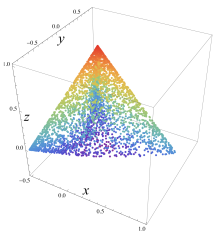
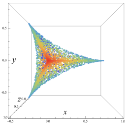
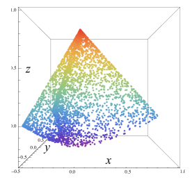
Figure 1: (Color online) Three views of the three-dimensional body, representing all possible values of the “conductance” matrix $M$ in the situation with the unbroken time-reversal symmetry.

The projection of this body onto the $(x,y)$ plane is shown in Fig.  2a. The limiting curve, bounding the possible values $(x,y)$, is called deltoid curve and is given parametrically by

$$x =(2\cos t+\cos 2t)/3,\quad y=(2\sin t-\sin 2t)/3,$$ (13)

with $t\in(0,2\pi)$.

Let us prove, that the shape in Fig.  2a is a deltoid. Introduce the notation $\tau=\cos\theta$, $u=\cos\xi$. Clearly, for fixed $\tau,u$ the boundary is reached at $\cos\psi=\pm 1$. In view of the symmetry ($\psi\to\pi-\psi$, $\theta\to\pi-\theta$), we may choose $\cos\psi=-1$ and seek the extrema of $M^{\prime}$ for both signs of $\tau$. We have

$$x =-\tfrac{1}{4}(1+\tau)(1+u^{2}+\tau(-3+u^{2})),$$ (14)

$$y =\tfrac{\sqrt{3}}{2}(-1+\tau^{2})u.$$

We find the extremum curve by i) fixing the direction $d(x/y)=0$ which gives the condition between $du$ and $d\tau$ and ii) expressing $du$ via $d\tau$ from this condition, we find the maximum of $x$, (simultaneously of $y$). It produces the parametric description of the limiting curve

$$x =\tfrac{1}{2}(3\tau^{2}-1),\quad y=\pm\tfrac{1}{2}(-1+\tau)\sqrt{3+6\tau-9\tau^{2}},$$ (15)

with the range of $\tau\in(-1/3,1)$, defined by positiveness of the square root in (15). This curve coincides with (13) after substitution $\tau=(1+2\cos t)/3$. Importantly, the above relation $x=\tfrac{1}{2}(3\tau^{2}-1)$ means that $z=0$ (i.e. $M_{11}=M_{22}$) for the limiting curve.

The cross section $y=0$ is shown in Fig.2b. The limiting curves are straight line $x+z=1$ (corresponding to zero conductance $G_{bb}$), and a parabola, given by

$$x =(3t-1)(t+1)/4,\quad z=(3t+1)(t-1)/4\;.$$ (16)

The lowest point $x=y=0$, $z=-1/3$ corresponds to maximum transparency of $Y$-junction, discussed below.

The projection onto the $(x,z)$ plane is shown in Fig.2c. This projection in fact corresponds to two cross-sections, delimited by parabola and straight line, and rotated by an angle $2\pi/3$ in three-dimensional space. The resulting contraction by a factor of $\sin(2\pi/3)=\sqrt{3}/2$ along the $x$-axis is taken into account, when drawing limiting curves here.

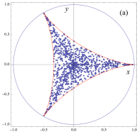
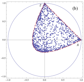
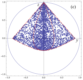
Figure 2: (Color online) (a) A top projection of the “tetrahedron”, showing the deltoid curve, denoted by a red line. The circumscribed circle is also shown. (b) The section $y=0$, corresponding to the symmetry between first and second wire; the bounding curve consist of a parabola and a straight line. (c) The projection onto the $(x,z)$ plane; one can see parabolic and straight lines, bounding the body, similarly to the cross section $y=0$, and shown by red lines.

Notice that there are only four points of “tetrahedron” which lie on the surface of the unit sphere in Fig. 1. They are $N=(0,0,1)$, $A_{3}=(1,0,0)$, $A_{1,2}=(-1/2,\pm\sqrt{3}/2,0)$ in coordinates $(x,y,z)$ and correspond to three detached wires, $N$, and (three times by) one detached wire, $A_{j}$, respectively. The related matrix $|S_{jk}|^{2}$ in (6) in cases $N,A_{1},A_{2},A_{3}$ has the form of permutation matrix, Eq. (20) below, with unity value for $p_{0},p_{1},p_{2},p_{3}$, respectively.

III.2 Magnetic flux and symmetry between two wires

In case of magnetic flux piercing the Y-junction and the additional symmetry between the wires 1 and 2, we have the relation $y=0$ in in Eq.  (10). At the formal level, however, this case is fully analogous to the one considered above. Indeed, the previous case corresponded to $\bar{\xi}=\xi$ and the present case reads $\bar{\xi}=\pi-\xi$. This difference amounts to a change $(x,y,z)\to(z,\eta,x)$, which means that the Fig. 1 and Fig.  2 having the same form in new axes.

The equations (14), (15) are now valid for $z,\eta$, and the limiting curve, bounding the values of conductance matrix, is again deltoid. Further, it happens at $x=0$, i.e. for the totally symmetric situation with respect to permutation of all three wires. Such particular case of total symmetry was considered earlier for interacting fermions in Nayak et al. (1999); Oshikawa et al. (2006).

Similarly, there are four points which lie on the surface of the unit sphere in coordinates $(z,\eta,x)$. They are the previous points $N,A_{3}$ and new ones $\chi_{\pm}=(-1/2,\pm\sqrt{3}/2,0)$. The latter points are the chiral fixed points corresponding to currents flowing from the wire $j$ to $j\mp 1$ and discussed in Oshikawa et al. (2006).

III.3 Geometrical interpretation

In this subsection we discuss the restrictions for the elements $M_{jk}$, which stem solely from the unitarity of S-matrix and do not involve particular properties of SU(3) group. We represent Eq. (17) in the form

$$M =\begin{pmatrix}\langle\tilde{\lambda}_{3}|\lambda_{3}\rangle,&\langle\tilde{\lambda}_{3}|\lambda_{8}\rangle\\ \langle\tilde{\lambda}_{8}|\lambda_{3}\rangle,&\langle\tilde{\lambda}_{8}|\lambda_{8}\rangle\end{pmatrix}\equiv\begin{pmatrix}a\cos\alpha,&b\cos\beta\\ a\sin\alpha,&b\sin\beta\end{pmatrix},$$ (17)

here the shorthand notation $\langle x|y\rangle=\tfrac{1}{2}Tr(x.y)$ was introduced.

It is seen, that the columns of $M$ are projections of $\lambda_{3}$ and $\lambda_{8}$ onto the hyperplane spanned by $\tilde{\lambda}_{3}$ and $\tilde{\lambda}_{8}$. We can think of the vectors $\vec{a}=\tilde{\lambda}_{3}\langle\tilde{\lambda}_{3}|\lambda_{3}\rangle+\tilde{\lambda}_{8}\langle\tilde{\lambda}_{8}|\lambda_{3}\rangle$ and $\vec{b}=\tilde{\lambda}_{3}\langle\tilde{\lambda}_{3}|\lambda_{8}\rangle+\tilde{\lambda}_{8}\langle\tilde{\lambda}_{8}|\lambda_{8}\rangle$. Each of the sets $\{\tilde{\lambda}_{j}\}$ and $\{\lambda_{j}\}$ with $j=0,\ldots 8$ forms the orthonormal basis for Hermitian matrices with the scalar product $\langle\cdot|\cdot\rangle$. Therefore we have $a^{2}=\sum_{j=3,8}|\langle\lambda_{3}|\tilde{\lambda}_{j}\rangle|^{2}\leq\sum_{j=1}^{8}|\langle\lambda_{3}|\tilde{\lambda}_{j}\rangle|^{2}=1$ and similarly $b^{2}\leq 1$. Notice that these inequalities follow from the unitarity of $S$, i.e. charge conservation.

Further, let us consider a unit vector $\vec{v}=\cos\gamma\,\lambda_{3}+\sin\gamma\,\lambda_{8}$ in the hyperplane spanned by $\lambda_{3}$ and $\lambda_{8}$. The projection of the circle $\gamma\in(0,2\pi)$ onto the plane $\{\tilde{\lambda}_{3},\tilde{\lambda}_{8}\}$ is given by $\vec{v}_{P}=\cos\gamma\,\vec{a}+\sin\gamma\,\vec{b}$ and should have the form of the ellipse. A simple calculation shows that the principal axes of this ellipse are given by

$$\cos^{2}\zeta_{\pm}=\tfrac{1}{2}({a^{2}+b^{2}})\pm\tfrac{1}{2}\sqrt{(a^{2}-b^{2})^{2}+4(\vec{a}.\vec{b})^{2}},$$ (18)

here $\vec{a}.\vec{b}=ab\cos(\alpha-\beta)$ Evidently, $\zeta_{-}$ is the dihedral angle between the hyperplanes $\{\tilde{\lambda}_{3},\tilde{\lambda}_{8}\}$ and $\{\lambda_{3},\lambda_{8}\}$. We also have an obvious geometrical inequality, $\cos^{2}\zeta_{+}\leq 1$, which can be written in the form

$$a^{2}+b^{2}\leq 1+a^{2}b^{2}\sin^{2}(\alpha-\beta)$$ (19)

and amounts to the statement that the eigenvalues of the non-negative matrix $M^{\dagger}.M=\begin{pmatrix}a^{2},&\vec{a}.\vec{b}\\ \vec{a}.\vec{b},&b^{2}\end{pmatrix},$ are less or equal to unity, $\|M^{\dagger}M\|\leq 1$.

III.4 Birkhoff-von Neumann theorem

Introducing $\bar{M}_{ij}=|S_{ij}|^{2}$ in Eq. (6), we write $G_{ij}=\delta_{ij}-\bar{M}_{ij}$. We have the property $\sum_{i}\bar{M}_{ij}=\sum_{j}\bar{M}_{ij}=1$, the matrices of this form are called doubly stochastic. For a vector space with elements $X_{i}$ we may form a linear combination of the form $\sum_{i}c_{i}X_{i}$. If each $c_{i}\geq 0$ and $\sum_{i}c_{i}=1$, then such combination is called convex combination.

The Birkhoff-von Neumann theorem states that an $n\times n$ matrix over $\Re$ is doubly stochastic if and only if it is a convex combination of permutation matrices.

A doubly stochastic matrix is called unistochastic if its elements can be represented as squared moduli of elements of unitary matrix. Any unistochastic matrix is contained in the set of doubly stochastic matrices, but not vice versa. In our case a general doubly stochastic matrix is a candidate for conductance matrix, but not all such matrices have a quantum-mechanical counterpart, $S-$matrix, i.e. they do not belong to unistochastic set. The analysis of $3\times 3$ unistochastic matrices, done in [Bengtsson et al., 2005; Zyczkowski et al., 2003], is relevant to our study. Particularly, it was shown, that the extreme points of unistochastic set are permutation matrices. The doubly stochastic property represents the classical Kirchhoff’s rule for the charge conservation, whose quantum-mechanical counterpart, the unitarity of $S-$matrix, necessarily involves the complex-valued quantities, except for extreme points and surfaces. A special role is played by two subsets of matrices of the form (cf. Eq.(16) in Agarwal et al. (2010))

$$\bar{M}_{1} =\begin{pmatrix}p_{0},&p_{4},&p_{5},\\ p_{5},&p_{0},&p_{4},\\ p_{4},&p_{5},&p_{0}\end{pmatrix},\quad\bar{M}_{2}=\begin{pmatrix}p_{1},&p_{3},&p_{2},\\ p_{3},&p_{2},&p_{1},\\ p_{2},&p_{1},&p_{3}\end{pmatrix}.$$ (20)

The above mentioned extreme cases correspond to $p_{i}=1$ for a given $i$, with all other $p_{i}=0$. These cases correspond to the above points $N$, $A_{1}$, $A_{2}$, $A_{3}$, $\chi_{+}$, $\chi_{-}$, for $i=0,\ldots 5$, respectively.

Explicitly, we have in general case of $M$, Eq. (10),

$$x =p_{3}-\tfrac{1}{2}(p_{1}+p_{2}),\quad y=\tfrac{\sqrt{3}}{2}(p_{1}-p_{2}),$$ (21)

$$z =p_{0}-\tfrac{1}{2}(p_{4}+p_{5}),\quad\eta=\tfrac{\sqrt{3}}{2}(p_{4}-p_{5}),$$

with $\sum_{i=0}^{5}p_{i}=1$.

The Birkhoff-von Neumann theorem does not imply a uniqueness of the convex combination. This becomes evident when we notice that $\bar{M}_{1}+\bar{M}_{2}=0$ for arbitrary $p_{0}$, if $p_{0}=p_{4}=p_{5}=-p_{1}=-p_{2}=-p_{3}$. For further illustration of this issue, consider the above additional condition of unbroken time-reversal symmetry $\eta=0$ which reduces the freedom in choice of parameters $p_{j}$, but not completely. The allowed values of $x,y,z$ for the doubly stochastic matrix $\bar{M}_{1}+\bar{M}_{2}$ of the above form fill the triangular bipyramid, which is the “classical” analog of the body shown in Fig.  1. This bipyramid is defined by its vertices $(x,y,z)$ at $(0,0,1)$, $(1,0,0)$, $(-1/2,\pm\sqrt{3}/2,0)$ and $(0,0,-1/2)$. The consideration of the case with magnetic flux, $y=0,\eta\neq 0$ is done similarly to above, due to obvious symmetry of Eq.  (21). We have the same bipyramid in coordinates $(z,\eta,x)$, as depicted in Fig. 3.

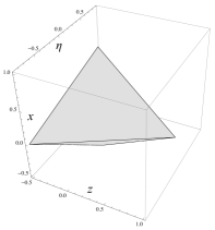
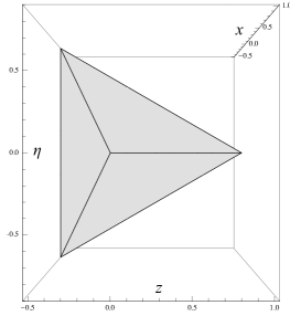
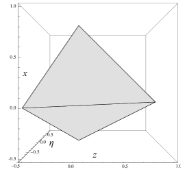
Figure 3: Three views of bipyramid, representing all possible values of classical “conductance” matrix $M$ in the symmetric situation ($y=0$ in Eq. (21)) with broken time-reversal symmetry.

Concluding this section, we make two observations. First, there are only six points, which lie on the surface of the unit four-dimensional sphere $(x,y,z,\eta)$. They are $N$, $A_{1,2,3}$, $\chi_{\pm}$ and this set is the same for doubly stochastic and unistochastic matrices. Second, the above inequality (19) can be cast into the form

$$\sqrt{x^{2}+y^{2}}+\sqrt{z^{2}+\eta^{2}}\leq 1.$$ (22)

This condition at $\eta=0$ represents two cones. Three straight lines, connecting $N$ and $A_{j}$ lie on the upper cone $z=1-\sqrt{x^{2}+y^{2}}$ and belong to the boundary of allowed values of conductance both for doubly stochastic and unistochastic sets. The lower cone, $z=-1+\sqrt{x^{2}+y^{2}}$, does not touch the above “tetrahedron” in both variants.

IV Discussion

IV.1 “Stability of the action”

Consider the energy, associated with the chiral fermionic densities in wires. For the ring of length $l$ the energy of the chiral current $\rho_{j}$ around the energy minimum is given by $\pi v_{F}l^{-1}(\rho_{j}-\rho_{j}^{(0)})^{2}$, see e.g. Aristov and Luther (2002); Aristov (2007) and references therein. Here $\rho_{j}^{(0)}$ is discrete variable (zero mode), measuring the number of particles moving at a given direction. Extending this formula to our situation, we have the energy of the incoming and outgoing d.c. currents per unit length

$$E_{in} =\pi v_{F}\sum_{j=1}^{3}\Big{(}l^{-1}\int_{-l}^{0}dx\,\langle\rho_{j,in}(x)\rangle\Big{)}^{2},$$ (23)

$$E_{out} =\pi v_{F}\sum_{j=1}^{3}\Big{(}l^{-1}\int_{0}^{l}dx\,\langle\rho_{j,out}(x)\rangle\Big{)}^{2}$$

with $l\to\infty$. This formula is written for the non-interacting fermions, and with some restrictions it can be used in the interacting case, as well. Such generalization is possible, e.g., when one considers the finite region of the interaction close to the origin, $|x|<L$, in Eq. (23). In this case the contribution of the interacting region $x\in(-L,L)$ in the semi-infinite leads to $E_{in,out}$ is negligible, and we can adopt the single-particle description of the outgoing states and the free-fermion relation between the applied voltage and the incoming current, $\langle\rho_{j,in}\rangle=\tfrac{e^{2}}{h}V_{j}$. The existence of the non-interacting leads beyond the finite region of interaction is important for the proper definition of $S$-matrix; it also leads to the absence of vertex corrections to conductance and the (correct) unity value of conductance of clean Luttinger liquid, as discussed at length in Aristov and Wölfle (2009). Here $\langle\rho_{j,in}\rangle$ stands for zero mode of the current, i.e. $\langle\rho_{j,in}(x)\rangle$ averaged over $x$ in (23). The linear response theory gives for the net current $I_{j}=\langle\rho_{j,in}\rangle-\langle\rho_{j,out}\rangle=\tfrac{e^{2}}{h}G_{jk}V_{k}=G_{jk}\langle\rho_{k,in}\rangle$. Therefore $\langle\rho_{j,out}\rangle=\bar{M}_{jk}\langle\rho_{k,in}\rangle$, with the above matrix $\bar{M}_{jk}=\delta_{jk}-G_{jk}=|S_{jk}|^{2}$. Notice that, by construction, $Tr(\bar{M})\geq 0$ for any $S$.

The energies (23) represent only a part of the energy of chiral fermions associated with the zero modes of the system. Indeed, from the general inequality $(\int fg)^{2}\leq(\int f^{2})(\int g^{2})$ we obtain $\pi v_{F}\Big{(}l^{-1}\int_{-l}^{0}dx\,\langle\rho_{j,in}(x)\rangle\Big{)}^{2}\leq\pi v_{F}l^{-1}\int_{-l}^{0}dx\,\langle\rho_{j,in}^{2}(x)\rangle\equiv E_{tot}$, where the last quantity is the total energy density in bosonization description. It is assumed, that the total energy of incoming fermions is given by the zero modes, $E_{in}=E_{tot}$.

Since the scattering is elastic, and a part of the energy $E_{in}$ after the scattering may become distributed among the excited particle-hole pairs (with non-zero momentum in appropriate description), one obtains the inequality $E_{in}\geq E_{out}$ which was called a stability condition in Oshikawa et al. (2006). This inequality means, that the eigenvalues of the non-negative matrix $\bar{M}^{\dagger}\bar{M}$, or equivalently $M^{\dagger}M$, are less or equal to unity.

We saw above, however, that the stability condition $\|M^{\dagger}M\|\leq 1$ follows automatically from the unitarity of $S$. The bosonization approach Bellazzini et al. (2007); Das and Rao (2008); Hou and Chamon (2008); Oshikawa et al. (2006) does not assume the unitarity of $S$-matrix (see below), but rather starts from the consideration of conductance matrix, $G$, or “current splitting” matrix, $\bar{M}$. As shown above, Eqs.  (17), (19), the restrictions for the parameters are

$$a^{2} \leq 1,\quad b^{2}\leq 1,$$ (24)

$$\cos^{2}(\alpha-\beta) \leq(a^{-2}-1)(b^{-2}-1)$$

The case considered in Ref. Oshikawa et al. (2006) reads in our notation as $a\cos\alpha=1-\tfrac{3}{2}G_{s}$, $a\sin\alpha=\tfrac{3}{2}\Delta$, $b=a$, $\beta=\alpha+\pi/2$. We see that the unitarity-related inequalities (24) reduce in this case to $(1-\tfrac{3}{2}G_{s})^{2}+(\tfrac{3}{2}\Delta)^{2}\leq 1$, which correspond to Eq. (11.13) in Oshikawa et al. (2006). At the same time, Figs.  2, 3 show that the bounding estimates (24), (22) are too weak.

IV.2 Abelian bosonization

Let us further comment on the nature of the inequality $E_{in}\geq E_{out}$ linking it to the bosonization approach. According to scattering states formalism described above and in Ref. Aristov and Wölfle, 2009, the components of outgoing density may include non-diagonal interference terms. For example, the appearance of $\lambda_{4}$ component in the outgoing current $\tilde{\rho}_{1}$ indicates the presence of combination $\psi^{\dagger}_{3}\psi_{1}+h.c.$. Contrary to the interpretation in Agarwal et al. (2010), the existence of such components of the density does not mean the power dissipation, as the scattering is elastic. The difference between the diagonal terms $\psi^{\dagger}_{j}\psi_{j}$ and off-diagonal terms $\psi^{\dagger}_{j}\psi_{i}$ ($i\neq j$) becomes more transparent, if we consider a non-equilibrium situation with voltage biases $V_{j}\neq 0$. In this case we should recall the existence of the rapidly oscillating exponents in the wave-function of the incoming fermion, $\psi_{j}(x)\sim\bar{\psi}_{j}(x)\exp ik_{Fj}x$, with Fermi momenta $k_{Fj}=k_{F}+V_{j}/v_{F}$; here we extracted the “smooth” part of the fermion operator $\bar{\psi}_{j}(x)$, see e.g. Gogolin et al. (1998). We see now that the diagonal terms $\psi^{\dagger}_{j}\psi_{j}$ in the outgoing current contain only smooth part of the density, whereas the off-diagonal part of the density contains “beats” in its profile, $\bar{\psi}^{\dagger}_{j}\bar{\psi}_{l}\exp i(V_{j}-V_{l})x/v_{F}$, cf. Ref.  Urban and Komnik (2008). Evidently, the off-diagonal terms vanish upon the averaging in (23), and this is exactly when the energy difference $E_{in}-E_{out}$ occurs. This difference is thus associated with the weight of the off-diagonal components of fermionic density, which may also include an analog of $2k_{F}$ Friedel oscillations.

The condition of exact equality $E_{in}=E_{out}$ indicates a possibility to fully express the outgoing currents in “smooth” components of incoming chiral densities. It means that, in the appropriate basis, the whole Hamiltonian is expressed entirely in smooth densities which is the essence of Abelian bosonization approach. Notice, that it is always possible to express the kinetic part of the action in terms of smooth densities in each of the semi-infinite wires. The difficulty in such a description arises at the moment of imposing a boundary conditions, which connect the smooth densities in different semi-wires. Oshikawa et al. (2006); Hou and Chamon (2008) Thus, for instance, a simpler case of the wire with a single impurity allowed a simple perturbative analysis only in two limiting cases of a clean wire and two detached semi-wires. Kane and Fisher (1992)

Evidently, the condition $E_{in}=E_{out}$ happens at $a=b=1$ and $\alpha=\beta\pm\pi/2$ in (17). We have two classes discussed in Agarwal et al. (2009, 2010); Bellazzini et al. (2009) namely

$$M_{1} =\begin{pmatrix}\cos\alpha,&\sin\alpha\\ -\sin\alpha,&\cos\alpha\end{pmatrix},$$ (25)

$$M_{2} =\begin{pmatrix}-\cos\alpha,&\sin\alpha\\ \sin\alpha,&\cos\alpha\end{pmatrix}.$$

(the form of $M_{1}$ in our notation has a direct correspondence with Eq. (10.17) in Oshikawa et al. (2006) ). In these cases $M$ is orthogonal, $M^{\dagger}M=1$, and one may promote the above equality for the averages to the operator form, $\rho_{j,out}=\bar{M}_{jk}\rho_{k,in}$. Then the commutation relations for the chiral fields, $[\rho_{j,in}(x),\rho_{k,in}(y)]=\tfrac{i}{2\pi}\delta_{jk}\delta^{\prime}(x-y)$, prescribed in bosonization, are fulfilled also for $\rho_{j,out}$.

In (Abelian) bosonization approach, the consistent perturbative analysis can be done only in a close vicinity of the RG fixed point, which is scale invariant or conformally invariant point in 1D. Bellazzini et al. (2007); Das and Rao (2008); Hou and Chamon (2008) The requirement for the above matrices (25) to represent the RG fixed point in bosonization leads to additional boundary conditions for three chiral densities at the Y-junction. These boundary conditions are expressed via a set of Neumann and Dirichlet boundary conditions for appropriate bosonic fields. An important observation, made in Ref. [Bellazzini et al., 2007], is that the trace of the matrix $\bar{M}$ at the fixed point is an integer number and equal to the number of Neumann conditions imposed. In simple words, $Tr(\bar{M})=1+Tr(M)=1+2z$, at the fixed point should be equal to the number of wires, detached from the $Y$ junction; it becomes rather obvious when we recall that $Tr(\bar{M})=|r_{1}|^{2}+|r_{2}|^{2}+|r_{3}|^{2}$. Evidently, the number of detached wires can be $0,1,3$, but not 2.

The fixed points discussed in bosonization approach include the above $N$ point, $M_{1}(\alpha=0)=\left(\begin{smallmatrix}1,&0\\ 0,&1\end{smallmatrix}\right),$ for three detached wires ; the $A_{3}$ point, $M_{2}(\alpha=0)=\left(\begin{smallmatrix}-1,&0\\ 0,&1\end{smallmatrix}\right),$ for the third wire detached, and also $M_{2}(\alpha=\pm 2\pi/3)=\left(\begin{smallmatrix}1/2,&\pm\sqrt{3}/2\\ \pm\sqrt{3}/2,&-1/2\end{smallmatrix}\right)$ for situations with the first and second wires detached, points $A_{1}$ and $A_{2}$. Two chiral fixed points $\chi_{\pm}$, present in the broken time-reversal case, are $M_{1}(\alpha=\pm 2\pi/3)=\left(\begin{smallmatrix}-1/2,&\pm\sqrt{3}/2\\ \mp\sqrt{3}/2,&-1/2\end{smallmatrix}\right)$; we have zero detached wires in this case.

However, formally there is seventh fixed point, first discussed in Nayak et al. (1999) and denoted as $D_{P}$ in Agarwal et al. (2010); Bellazzini et al. (2009); Das and Rao (2008); Oshikawa et al. (2006). It is given by $M_{1}(\alpha=\pi)=\left(\begin{smallmatrix}-1,&0\\ 0,&-1\end{smallmatrix}\right)$. From our Eq. (9) we have $G_{aa}=1$, $G_{bb}=4/3>1$, i.e. the value of one-terminal conductance $G_{bb}$ at the $D_{P}$ point is larger than the maximum value of unity for the non-interacting situation. This enhanced value of conductance was interpreted as the signature of Andreev reflection and multiparticle scattering at the Y-junction. Nayak et al. (1999); Oshikawa et al. (2006) We observe that for $D_{P}$ point one has $Tr(\bar{M})=-1$, and it contradicts the charge conservation law both in quantum mechanical and classical formulation, at least for free fermions. Indeed, we should have $Tr(\bar{M})\geq 0$ for any unitary $S$-matrix, and for any doubly stochastic matrix, representing Kirchhoff’s rule.

One might argue, that our analysis, performed for free fermions, is inapplicable to the case of strongly interacting regime, where the importance of $D_{P}$ point was emphasized. It was predicted in Nayak et al. (1999); Oshikawa et al. (2006) that the fixed point $D_{P}$ becomes stable at strong attraction between fermions, $g>3$, whereas it is unstable at weaker interaction, $g<3$ (cf. also Bellazzini et al. (2009)). The existence of $D_{P}$ point, however, was not ruled out for any values of interaction and, particularly, in the free fermion limit, $g\to 1$. The inspection of formulas (10.29)–(10.31) in Oshikawa et al. (2006) and Eq. (62) in Bellazzini et al. (2009) for the scaling dimension of leading perturbations confirms it. Therefore we have to conclude, that the discussed boundary for physical conductances was not so far detected by means of conventional bosonization. One possibility here, potentially favorable for the existence of $D_{P}$ point, is that this boundary changes with the Luttinger parameter $g$ and thus should be separately discussed for each value of $g$. Another possibility, supported by our analysis in Aristov et al. (2010); unpub , is that the boundary determined for free fermions remains the same for any interaction strength. Particularly, any physical RG fixed point belongs to this boundary, while the above Fig. 2b and the Fig. 5 in Aristov et al. (2010) depict the same parabola. From this latter viewpoint, the discussed $D_{P}$ point lies outside the physical domain and is not connected with the inside of the body in Fig.  1 by any RG flow. As was already mentioned in Sec. IV.1, we assume the infinite non-interacting leads beyond the finite region of interaction, which setup provides the proper definition of $S$-matrix and vanishing vertex corrections to conductance.

Based on the above observations I make a following stronger conjecture. The two classes (25) do not represent any physical realization of $Y$-junction, except for six points listed above and corresponding to permutation matrices in Eq. (20). These six points are the extreme points of the four-dimensional body, whose three-dimensional projections are shown in Fig.  1. All other physical realizations of the $Y$-junction lead to values $(x,y,z,\eta)$ lying strictly inside the four-dimensional unit sphere, Eqs. (22), (24), whose surface is needed as a starting point in bosonization. Thus the Abelian bosonization study of the $Y$-junction can be performed at six RG fixed points only, at the vertices of the body in Fig.  1. If the RG fixed point occurs at the boundary of this body instead, then it is unsuitable for conventional bosonization analysis. It should be stressed again, that this conjecture is based on the present free-fermion analysis and on the results of perturbative two-loop RG treatment valid for relatively weak interaction. Aristov et al. (2010) The case of strong interaction is to be discussed elsewhere. unpub

IV.3 Larger-$N$ junctions

The observations reported in this paper for the Y-junction, can be generalized for a larger number of semi-wires, $N>3$, attached to one spot. The $S$-matrix in this case will be given by a finite rotation matrix in $SU(N)$ group, and the squares of its entries form the unistochastic matrix $\bar{M}$. The set of all such $\bar{M}$ lies within a set of bistochastic matrices, whose extreme points are $N!$ permutation matrices, according to the Birkhoff-von Neumann theorem. These permutation matrices describe the physical situations when some of the wires are detached from the central spot, whereas the other semi-wires form either ideal wires (in case of pairwise partial permutations) or chiral groups, involving three or larger number of semi-wires. For example, for $N=4$ (see also Bengtsson et al. (2005); Zyczkowski et al. (2003)) we obtain $24$ matrices, which correspond to 4 detached wires (one point in phase space), 2 detached wires and one full wire (six points), one detached wire and a chiral group of three semi-wires (eight points), two full wires (three points), and a chiral group of four semi-wires (3!=6 points). These points lie on an appropriate unit hyper-sphere and thus are suitable as fixed points in Abelian bosonization. We note also that the particular case of fully symmetric $S$-matrix and fully symmetric interacting wires can be solved within TBA approach Egger et al. (2003) for any $N$, because the high symmetry effectively reduces this case to $N=2$. The latter approach allows to consider the RG fixed point, corresponding to the perfectly transmitting junction ($z=-1/3$ in our above case $N=3$).