Asymmetric spin-1/2 two-leg ladders

Abstract

We consider asymmetric spin-1/2 two-leg ladders with non-equal antiferromagnetic (AF) couplings $J_{\|}$ and $\kappa J_{\|}$ along legs ($\kappa\leq 1$) and ferromagnetic rung coupling, $J_{\perp}$. This model is characterized by a gap $\Delta$ in the spectrum of spin excitations. We show that in the large $J_{\perp}$ limit this gap is equivalent to the Haldane gap for the AF spin-1 chain, irrespective of the asymmetry of the ladder. The behavior of the gap at small rung coupling falls in two different universality classes. The first class, which is best understood from the case of the conventional symmetric ladder at $\kappa=1$, admits a linear scaling for the spin gap $\Delta\sim J_{\perp}$. The second class appears for a strong asymmetry of the coupling along legs, $\kappa J_{\|}\ll J_{\perp}\ll J_{\|}$ and is characterized by two energy scales: the exponentially small spin gap $\Delta\sim J_{\perp}\exp(-J_{\|}/J_{\perp})$, and the bandwidth of the low-lying excitations induced by a Suhl-Nakamura indirect exchange $\sim J_{\perp}^{2}/J_{\|}$. We report numerical results obtained by exact diagonalization, density matrix renormalization group and quantum Monte Carlo simulations for the spin gap and various spin correlation functions. Our data indicate that the behavior of the string order parameter, characterizing the hidden AF order in Haldane phase, is different in the limiting cases of weak and strong asymmetry. On the basis of the numerical data, we propose a low-energy theory of effective spin-1 variables, pertaining to large blocks on a decimated lattice.

I Introduction

Recent progress in nanotechnologies, molecular electronics and quantum computing reinvigorated the interest to low-dimensional systems. Special attention has focused during recent years on quantum dots, arrays of coupled quantum dots, Lee et al. (2002) quantum wires, spin chains or ladders. Another class of physical systems where low-dimensionality can be achieved is ultra-cold gases in optical lattices, Bloch et al. (2008); Giamarchi (2010) which form good prototype systems for investigation of many strongly-correlated effects, such as metal-insulator transition, low-dimensional superconductivity or formation of various density-wave states. The advantage of these systems is the high controllability of model parameters with external fields and preparation conditions.

Many of these systems display low-energy feature that fall outside the standard behavior predicted by Landau’s Fermi liquid or symmetry breaking theories. In particular, the existence of a non-local (string) order parameter is proven, both analytically Shelton et al. (1996) and numerically Schollwöck et al. (1996), to be a characteristic feature of several classes of one-dimensional (1D) and quasi-1D systems. Gogolin et al. (1998); Giamarchi (2003) Such non-local order parameters are topologically protected against any local perturbations. The nature of these order parameters and the connection to topological invariants Gogolin et al. (1998) is well understood Affleck (1989) for spin chains with $S\geq 1$. For instance, the Haldane conjecture Haldane (1983) proposed more than 20 years ago states that the properties of $SU(2)$ symmetric antiferromagnetic (AF) spin-$S$ Heisenberg chains differ for integer and half-integer spins. The excitations in the AF Heisenberg chains with half-integer spins are gapless Affleck and Lieb (1986) whereas in the integer spin case, a gap is present. The pure one-dimensional (1D) AF spin-$1/2$ Heisenberg chain can be mapped onto a Luttinger liquid which allows an exact bosonization treatment, resulting in a well understood gapless phase. Affleck and Lieb (1986) In contrast, for the AF spin-$1$ Heisenberg chain it is widely accepted that the excitations exhibit a gap, thanks to extensive numerical Nightingale and Blöte (1986); Takahashi (1989); White and Huse (1993); Deisz et al. (1993); Golinelli et al. (1994); Todo and Kato (2001) and experimental Honda et al. (1998); Zheludev et al. (2003) analysis.

The present understanding of systems of coupled identical $S=1/2$ chains (spin ladders) is based on its similarities to larger-spin chains. This similarity allows the one-to-one translation of Haldane’s conjecture, originally formulated for large-spins chain, onto spin-1/2 ladders with an odd or even number of identical legs. The usual assumption about the equivalence of the individual chains constituting the ladder, is referred below as a symmetric ladder situation. While the behavior of symmetric ladders has been thoroughly investigated, both theoretically and experimentally Dagotto and Rice (1996); Gogolin et al. (1998), the case of spin ladders with inequivalent legs (asymmetric ladders) is less understood. The behaviour of the spin gap, in particular for the case of a single chain coupled to nearly free spins (“dangling spins”) was recently discussed in Kiselev et al. (2005a, b); Essler et al. (2007); Brünger et al. (2008), but no firm conclusions about the gap scaling in the weak coupling regime were made there.

In this work, we consider the Spiral Staircase Heisenberg ladder (SSHL), consisting of of two unequal antiferromagnetically coupled spin-$1/2$ chains with a ferromagnetic (FM) rung coupling $J_{\bot}$. Geometrically, this model may be understood as a continuous twist deformation of an isotropic 2-leg ladder with interleg coupling $J_{\|}$ along leg $1$ by an angle $\theta$ (see Fig. 1). As a result of the deformation, the coupling between neighboring sites along leg 2 is rescaled to the form $J_{\|}\cos^{2}\left(\theta/2\right)$ leading to the Hamiltonian (1) below.

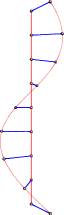
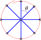
Figure 1: (Color online) (a) Sketch of the Spiral Staircase Heisenberg Ladder. (b) View of the system from the top. For $\theta=0$ the model corresponds to the standard antiferromagnetically coupled spin-$1/2$ Heisenberg ladder with FM rung coupling. The case $\theta=\pi$ corresponds to the 1D $SU(2)$ symmetric single-pole ladder model.

As is known from the seminal bosonization work of Shelton, Nersesyan and Tsvelik, Shelton et al. (1996) the FM coupling of AF spin chains induces a Haldane gap proportional to $J_{\perp}$ for weak interleg couplings. However, when the spin velocity on one of the legs vanishes the bosonization method fails as seen from the fact that a simple formulation of the continuum limit, on which the bosonization approach relies, is inhibited. Alternative approaches, such as using other analytical or numerical methods, are then demanded. Beside the theoretical interest, an experimental motivation comes from the fact that the single-pole ladder model at $\theta=\pi$ can been used for modeling a stable organic biradical crystal PNNNO. Hosokoshi et al. (1999)

In our previous work (Ref. Brünger et al., 2008), we used the quantum Monte Carlo simulations for investigation of asymmetric ladders. We demonstrated a non-zero value of string order parameter for the whole family of such ladders, which confirmed that the system is in a Haldane phase. We also presented numerical evidence for the smaller energy scale, $J_{\perp}^{2}/J_{\|}$, associated with Suhl-Nakamura interaction (see below). Numerical results for the spin gap were also judged compatible as vanishing as $J_{\perp}^{2}/J_{\|}$, even though a faster decay could not be ruled out. These results were consistent with the flow equation calculations of Essler and coworkers Essler et al. (2007).

In the present paper we show, that the spin gap changes its behavior at small $J_{\perp}\ll J_{\|}$ from $\Delta\sim J_{\perp}$ in the symmetrical ladder case to $\Delta\sim J_{\perp}\exp(-J_{\|}/J_{\perp})$ in the single-pole ladder case. Alternatively, we may think about rungs with a fixed exchange coupling $J_{\perp}$, while the leg exchange increases gradually. We observe that the small-$J_{\|}$ behavior $\Delta\sim J_{\|}$ is the same for all asymmetric ladders, but that important differences appear in the limit $J_{\|}\to\infty$. The symmetrical ladder displays a saturation of the spin gap, $\Delta\sim J_{\perp}$, while the gap in the single-pole ladder reaches a maximum at $J_{\|}\sim J_{\perp}$ and exhibits exponential suppression beyond that scale, according to the above formula.

The plan of the paper is as follows. We introduce the model and important definitions in Section II, where we also provide simple qualitative considerations. Particularly, we explain here the importance of Suhl-Nakamura (SN) indirect exchange between dangling spins in the single-pole situation.

We propose analytical approaches to our model in Section III. In Section III.1 we develop a theory, incorporating spin-wave analysis, SN interaction and Kadanoff’s decimation procedure, which satisfactorily describes the whole body of numerical data presented below. We stress that several quantities are extracted from the numerical data and plotted specifically for comparison with the predictions of this effective theory. The unusual slow saturation of the spin gap value at large $J_{\perp}$ is discussed in Section III.2.

In Section IV we describe the results of our extensive numerical investigations of the problem. Section IV.1 discusses exact diagonalization (ED) results. The appearance of a SN energy scale $J_{\bot}^{2}/J_{\|}$ is shown here. Given the long-range character of the SN interaction which require large systems to be appreciated, we resort to large scale quantum Monte Carlo (QMC) simulations in the next subsection. With this approach, we investigate the form of the spin correlation functions in Section IV.2, compute the spin gap in Section IV.3 as well as the string order parameter in Section IV.4, characteristic of the Haldane phase. The most challenging case of the single-pole ladder gives rise to the largest uncertainties for the spin gap, and we focus on this system with the use of the DMRG method, as described in Section IV.5. The DMRG results do not give a principal advantage over QMC findings, but they provide a strong independent verification of the observed form of the spin gap, namely an exponential suppression at small $J_{\perp}$.

In Appendix A, we analyze the qualitative changes in the spectra of symmetric and single-pole ladders within a Jordan-Wigner mean-field calculation. Technicalities of spin-wave theory for long-range interaction are given in Appendix B. We finally present our conclusions in Section V.

II problem setup and qualitative considerations

We study the low-energy physics of the SSHL system, characterized by the following Hamiltonian:

$${\mathcal{H}} = J_{\|}\sum_{i}\left({\mathbf{S}}_{1,i}\cdot{\mathbf{S}}_{1,i+1}+\cos^{2}\left(\tfrac{\theta}{2}\right){\mathbf{S}}_{2,i}\cdot{\mathbf{S}}_{2,i+1}\right)$$ (1)

$$- J_{\perp}\sum_{i}{\mathbf{S}}_{1,i}\cdot{\mathbf{S}}_{2,i}\,\,.$$

Here, ${\mathbf{S}}_{\alpha,i}$ is a spin-$1/2$ operator acting on leg $\alpha$ and lattice site $i$ and $J_{\|}>0$ sets the energy scale. The single-pole ladder model Kiselev et al. (2005a); Aristov et al. (2007); Brünger et al. (2008) corresponds to $\theta=\pi$.

It is convenient to reformulate the model Eq.(1) in terms of new variables,

$${\mathbf{S}}_{i}={\mathbf{S}}_{1,i}+{\mathbf{S}}_{2,i}\,\,,\quad{\mathbf{R}}_{i}={\mathbf{S}}_{1,i}-{\mathbf{S}}_{2,i}\,\,,$$ (2)

defined on the rung. The Hamiltonian then reads

$${\mathcal{H}} = \frac{J_{\|}}{4}\sum_{i}\left(1+\cos^{2}\left(\tfrac{\theta}{2}\right)\right)\left({\mathbf{S}}_{i}\cdot{\mathbf{S}}_{i+1}+{\mathbf{R}}_{i}\cdot{\mathbf{R}}_{i+1}\right)$$ (3)

$$+ \frac{J_{\|}}{4}\sum_{i}\sin^{2}\left(\tfrac{\theta}{2}\right)\left({\mathbf{S}}_{i}\cdot{\mathbf{R}}_{i+1}+{\mathbf{R}}_{i}\cdot{\mathbf{S}}_{i+1}\right)$$

$$- \frac{J_{\bot}}{4}\sum_{i}\left({\mathbf{S}}^{2}_{i}-{\mathbf{R}}^{2}_{i}\right)\,\,.$$

The set of operators ${\mathbf{S}}_{i}$ and ${\mathbf{R}}_{i}$ fully defines the $o_{4}$ algebra. Kiselev et al. (2005b, a)

Let us define the retarded spin response function in the ladder situation

$$\chi_{jl}(q,\omega) =-i\int_{0}^{\infty}dt\sum_{n}e^{i\omega t-iqn}\langle[{S}^{z}_{j,1}(t),{S}^{z}_{l,1+n}]\rangle,$$ (4)

$$=\int d\omega^{\prime}\frac{S_{jl}(q,\omega^{\prime})\,}{\omega-\omega^{\prime}+\mathrm{i}0}$$

with $j,l=1,2$. At zero temperature the dynamic structure factor (spectral weight), given by $S_{jl}({q},\omega)=-\pi^{-1}{\rm Im}\,\chi_{jl}(q,\omega)$ is represented as

$$S_{jl}({q},\omega) =\sum_{n}\langle 0|{S}^{z}_{l}(q)|n\rangle\langle n|{S}^{z}_{j}(-q)|{0}\rangle\delta(E_{n}-E_{0}-\omega)$$ (5)

where $|{0}\rangle$ stands for the ground state with the energy $E_{0}$, the sum runs over all eigenstates $|n\rangle$ of the Hamiltonian with energies $E_{n}$ and ${S}^{z}_{l}(q)$ is a Fourier transform of ${S}^{z}_{ln}$. We also define the symmetrized combinations,

$$S({q},\omega) =S_{11}({q},\omega)+S_{22}({q},\omega)+S_{12}({q},\omega)+S_{21}({q},\omega),$$ (6)

$$R({q},\omega) =S_{11}({q},\omega)+S_{22}({q},\omega)-S_{12}({q},\omega)-S_{21}({q},\omega),$$

which are response functions for operators $S^{z}$ and $R^{z}$ in (2), respectively.

Below we also use imaginary time correlation functions

$$\langle{S}^{z}_{q}(\tau){S}^{z}_{-q}(0)\rangle =\int d\omega\,\frac{e^{-\tau\omega}}{1-e^{-\beta\omega}}S(q,\omega)$$ (7)

$$\langle{R}^{z}_{q}(\tau){R}^{z}_{-q}(0)\rangle =\int d\omega\,\frac{e^{-\tau\omega}}{1-e^{-\beta\omega}}R(q,\omega)$$

with $\beta=1/T$.

Let us now qualitatively discuss the situation. In the strong coupling region, $J_{\bot}/J_{\|}\rightarrow\infty$, and for all possible twist angles $\theta$ triplets on the rungs become more and more favorable such that the Hamiltonian of Eq. (3) reduces to a pure spin-1 effective Hamiltonian:

$${\mathcal{H}}_{\mathrm{eff}} = J_{\mathrm{eff}}\sum_{i}{\mathbf{S}}_{i}\cdot{\mathbf{S}}_{i+1}$$ (8)

$$J_{\mathrm{eff}} = \tfrac{J_{\|}}{4}\left(1+\cos^{2}(\theta/2)\right)\,\,.$$

In units of effective coupling $J_{\mathrm{eff}}$ (and thus irrespective of the twist angle) the spin gap of our model scales to the Haldane gap $\Delta_{H}/J_{\mathrm{eff}}=0.41048(6)$. Todo and Kato (2001)

In the weak coupling region the situation is more delicate and depends on the twist $\theta$. Let us discuss here the limiting cases.

For the symmetric ladder, $\theta=0$, the gap opens as $\Delta\sim J_{\perp}$, as obtained by bosonization and also qualitatively reproduced in the simplified mean-field picture below. For the fully asymmetric single-pole ladder $\theta=\pi$ the mean-field calculation predicts a sub-linear behavior of the gap $\Delta\sim J_{\perp}^{2}/J_{\|}$. The bosonization treatment becomes problematic in this case, as we cannot apply the continuum approach to the chain of dangling spins attached to the main leg. The assumption of the finite Fermi (sound) velocity in the subsystem breaks down and $J_{\perp}$ cannot be used as a perturbation in the implicitly assumed hierarchy of scales $J_{\perp}\ll J_{\|}\cos^{2}(\theta/2)<J_{\|}$.

Instead, we should start with the picture of a degenerate band of dangling spins, whose degeneracy is lifted by indirect exchange between these spins through the main leg. This phenomenon is known as a Suhl-Nakamura interaction Suhl (1957); Nakamura (1958); Aristov et al. (1994) for the case of a dilute system of extra spins in a magnetic host. It has a direct analogy with the RKKY interaction where itinerant electrons mediate a long range spin-spin interactions between localized spins (see Ref. Aristov, 1997 and references therein). In second order perturbation theory the SN interaction reads:

$$J_{SN}\propto J^{2}_{\perp}\chi({q},\omega=0)\,\,,$$ (9)

where $\chi({q},\omega=0)$ is the spin susceptibility of the spin-$1/2$ Heisenberg chain. We thus arrive at a similar energy $J_{\perp}^{2}/J_{\|}$ but now it stands for the SN-induced bandwidth, not for the spin gap.

It is important to remark that both the mean-field treatment and the SN energy scale estimate provide us only with an upper bound for the gap value, $J_{\perp}^{2}/J_{\|}$. However this is likely a strong overestimation as quantum fluctuations, which are important in 1D, are not accounted for. In Sec.  III we present analytic arguments in favor of a gap vanishing faster than with a power law. In Sec.  IV we show, that the whole body of numerical data supports this scenario.

III Analytic approaches and interpretation

In most cases, it is instructive to map the system of spins onto a system of 1D spinless fermions. We show in Appendix A, that such Jordan-Wigner transformation and a subsequent mean-field theory analysis predict qualitative changes in the behavior of the gap with $\theta$. Particularly, Eq.  (41) there indicates that the prefactor in the linear law, $\Delta\sim J_{\perp}$, diminishes with decreasing $\cos\tfrac{\theta}{2}$, and that in the extreme case of single-pole ladder ($\cos\tfrac{\theta}{2}\to 0$), the gap vanishes faster than $|J_{\perp}|$. These observations are qualitatively confirmed by our numerical simulations. At the same time, the attempt to compare the mean-field results for the fermionic theory with the gap extracted from QMC data shows that the mean-field theory overestimates the gap by an order of magnitude.

In view of this fact, we perform a different type of analysis in the next subsections.

III.1 Decimated blocks and effective spins

Below we propose a scenario, which assumes different behavior of spin dynamics at high and low energies, as separated by the scale $J_{\perp}$. This scenario is explicitly formulated for the single-pole ladder, which represents the most intriguing and difficult case, as seen in the numerics. The extension of this scenario to $\theta\neq\pi$ is also briefly discussed at the end of this subsection. The proposed theory allows to semi-quantitatively explain all features observed in the large-scale QMC and DMRG studies.

For the high energies in consideration $\epsilon>J_{\perp}$, the dangling spins should be considered as freely attached to the main chain. These energies correspond to short times, $t<J_{\perp}^{-1}$, and distances, $x<J_{\|}/J_{\perp}$. Alternatively, one may think in terms of a higher temperature $T>J_{\perp}$, which smears all fine features of the spectrum and leads to exponential decay of correlations beyond the temperature correlation length $\sim J_{\|}/T$. The inverse length scale along the leg, $\xi^{-1}$, associated with the crossover to the low-energy dynamics is defined by the relation $J_{\perp}\sim\xi^{-1}J_{\|}$, showing that soft spinon excitations in the HAF spin-1/2 chain, with momenta $q\lesssim\xi^{-1}$ are strongly intertwined with triplet-singlet transitions on the rungs.

At these shorter time scales the classification in terms of singlet and triplet on the rung is not very appropriate. It means that the dangling spins are viewed as almost decoupled from the main chain: the situation is best described in terms of dangling spins coupled to each other by the Suhl-Nakamura interaction. The long-range character of SN interaction leads to an almost flat dispersion of the magnon excitations in the subsystem of dangling spins, the estimated SN energy scale not exceeding the crossover energy $J_{\perp}$.

At smaller energies, $\epsilon<J_{\perp}$, a picture of already formed triplets on the rungs is more appropriate. The discussion of the dynamics reduces to the rotations of the effective spins $S=1$. Further, these rung triplets are interlaced by the leg interaction into large effective spin blocks of size $\xi$. Despite a possibly large spatial size of the block, the AF character of the main leg interaction selects the smallest possible total spin state of this block. Discarding the non-magnetic singlet, we focus on the block triplet state, i.e., when $\xi$ spins $S=1$ are combined into a new effective spin $S=1$ of the block. As a result, we have a model with nearest-neighbors interaction between large blocks. Such a model should display a Haldane gap, whose value can be determined from usual arguments.

Let us start with the shorter distances and higher energies. In this case the SN interaction between dangling spins $S_{2,i}$ and $S_{2,i+x}$ has the form $V(x)S_{2,i}S_{2,i+x}$ with

$$V(x)=J_{\perp}^{2}\int\frac{dq}{2\pi}\chi(q,\omega=0)e^{iqx}\sim J_{\perp}^{2}/J_{\|}(-1)^{x}\ln(\xi/x)$$ (10)

with $\chi(q,\omega)$ is the response function for the HAF $S=1/2$ model. Gogolin et al. (1998) For our purposes it suffices to approximate $\chi(q,\omega=0)$ by $J_{\|}^{-1}|\cos(q/2)|^{-1}$. The $1/q$ singularity near $q=\pi$ shows that $V(x)$ is sign-reversal and logarithmically decaying with distance, $V(x)\sim(-1)^{x}\ln(\xi/x)$. The scale $\xi$ in the argument of the logarithm,appears here as a parameter which will be further determined by a self-consistency criterion. Technically it is assumed that the allowed energies, $\omega_{q}$, of the spin-wave continuum are restricted from below, $\omega_{q}\gtrsim J_{\|}/\xi$.

A chain of dangling spins, coupled by long-range SN interactions (10), behaves differently from the standard HAF model with nearest-neighbor interaction. A simple spin-wave analysis is then indispensable here. Such an analysis cannot give a correct form of correlation functions, but delivers a qualitative information about the spectrum. Affleck and Oshikawa (1999); Aristov and Kiselev (2004)

Using the formulas listed in Appendix B we conclude that the spin-wave spectrum in the system of dangling spins is given by the expression $\omega_{k}=\sqrt{g_{k}g_{k+\pi}}$, with $g_{k}=V(\pi)-V(\pi+k)$. Approximating the range function $V(\pi+k)\simeq(J_{\perp}^{2}/J_{\|})(\sin^{2}(k/2)+\xi^{-2})^{-1/2}$ we have

$$\omega_{k+\pi}\simeq (J_{\perp}^{2}/J_{\|})\xi\sqrt{1-(1+\xi^{2}\sin^{2}(k/2))^{-1/2}}$$ (11)

$$\simeq (J_{\perp}^{2}/J_{\|})\xi,\quad|k|\gg\xi^{-1}$$

$$\simeq (J_{\perp}^{2}/J_{\|})\xi^{2}|k|,\quad|k|\ll\xi^{-1}$$

Next we make the natural assumption that the top of the SN-induced band coincides (at least by the order of magnitude) with the logarithmic low energy cutoff introduced above, leading to $(J_{\perp}^{2}/J_{\|})\xi\sim J_{\|}/\xi$ or

$$\xi\sim J_{\|}/J_{\perp}$$ (12)

Remarkably, this estimate shows that the low-energy spin-wave dispersion (11) is characterized by the same velocity $\omega_{k+\pi}\sim J_{\|}|k|$ as the higher-energy excitations in the main leg. This is despite the fact that, strictly speaking, the low energies $\epsilon\ll J_{\perp}$ should be considered with a different approach as proposed below. Notice that the described spectrum resembles a simple picture of hybridization between the linear spectrum and initially degenerate band at non-zero energy $\sim J_{\perp}$, with the crossing level repulsion phenomenon.

At small energies $\epsilon\ll J_{\perp}$, we expect that the picture of spinons (in the main leg) scattering on the dangling spins, becomes inadequate. The dynamics of spins on the rung is characterized in terms of soft triplet dynamics, while the transitions to singlet state with the (now) large energy $J_{\perp}$ are discarded. On the same ground, we discard spin-wave continuum excitations with energies $\epsilon\gtrsim J_{\perp}\sim J/\xi$, i.e., the description now has changed from the individual sites along the leg to entire blocks of length $\xi$. We may thus think in terms of the effective spin $S=1$ on the rung, and these individual spins $S=1$ are antiferromagnetically coupled to each other in the large block.

Furthermore, we can characterize the whole block $\xi$ of spins 1 by its lowest non-trivial multiplet, a spin 1 again. However now it is an object defined at a much larger spatial scale. The trivial low-energy multiplet in such $\xi$-block is a spin-singlet state, which obviously drops out from the soft spin dynamics.

The typical energy spacing between the resulting spin-triplet of the $\xi$-block and the higher multiplets is estimated again as $J_{\|}/\xi\sim J_{\perp}$. We expect that this lowest triplet state is non-degenerate, i.e. other triplets are higher in energy. Below we refer to this lowest triplet state as $\xi$-triplet.

We note in passing that the estimate $\xi\sim J_{\|}/J_{\perp}$ follows also from the argument presented in Ref. Essler et al., 2007. It was suggested there that the spinons, propagating along the main leg by distance $m$ and characterized by a typical energy $J_{\|}$, break the pre-formed rung triplets resulting in an energy cost $\sim mJ_{\perp}$. The resulting confining potential should, in principle, restrict the motion of spinons to distances $\sim J_{\|}/J_{\perp}$.

Our way of constructing $\xi$-triplet resembles Kadanoff’s decimation procedure in the description of critical phenomena. Huang (1987) The new lattice of large blocks contains spins 1, which are denoted below by $S_{\xi,n}$ (here $n$ numbers a position in a new lattice) and are coupled to each other by a nearest-neighbor interaction. In fact, only the edge spins of each $\xi$ block are responsible for this interaction. Adopting the notation that the weight of these edge spins in the $\xi$-triplet is $w_{1}\ll 1$ at $\xi\gg 1$ (see below), we write explicitly for odd $\xi$

$$S_{1,j}^{\alpha}=w_{1}S_{\xi,n}^{\alpha}(-1)^{j+n}$$ (13)

where $n=\lfloor j/\xi\rfloor$ and $\lfloor\ldots\rfloor$ stands for the floor function. Similarly, $S_{2,j}^{\alpha}=w_{2}S_{\xi,n}^{\alpha}(-1)^{j+n}$. The phase $(-1)^{j}$ accounts for the AF character of the contributing spins in the $\xi$-block and the additional phase shift $(-1)^{n}$ is introduced to restore the translational invariance in the blocks picture.

The definition of the above weight $w_{j}$ is as follows. Assume that the lowest multiplet in the $\xi$-block is a triplet $|T,m\rangle$, spanned by the spin-1 operators $S_{\xi,n}^{\alpha}$. Then, up to a sign, the edge operators of the block act as

$$\langle T,m^{\prime}|S_{1,j}^{\alpha}|T,m\rangle=w_{1}\langle T,m^{\prime}|S_{\xi,n}^{\alpha}|T,m\rangle,$$ (14)

and similarly for the weight $w_{2}$ of $S_{2,j}^{\alpha}$. The block Hamiltonian on the decimated lattice reads

$$\sum_{n}J_{\|}S_{1,n\xi}S_{1,n\xi+1}\to\sum_{n}w_{1}^{2}J_{\|}S_{\xi,n}S_{\xi,n+1}$$ (15)

with $n=1,\ldots L/\xi$. This model should exhibit a Haldane gap, but the value of this gap is strongly diminished.

Employing a standard albeit simplified approach used in the original Haldane paper, we apply the linearized spin-wave theory outlined in Appendix B and obtain the magnon dispersion, $\omega_{k}=4w_{1}^{2}J_{\|}\sin(k)$, where $k$ is the wave vector on the decimated lattice $k=2\pi n(\xi/L)$ with $n=1,2,\ldots$. It implies that the velocity of the lowest-lying excitations with respect to the real lattice is given by $\tilde{v}=4w_{1}^{2}\xi J_{\|}$. With the plausible assumption that this low-energy estimate coincides with the high-energy one, we obtain $\tilde{v}\sim J_{\|}$ and hence $w_{1}^{2}\sim\xi^{-1}$. Notice that it corresponds to a bandwidth $4w_{1}^{2}J_{\|}\sim J_{\perp}$, in accordance with Eq. (11).

We require that the zero-point magnon fluctuations cancel the local magnetization in the usual formula $S_{1,j}^{z}=1/2-S_{1,j}^{-}S_{1,j}^{+}$, i.e., we write $\langle S_{1,j}^{-}S_{1,j}^{+}\rangle=1/2$. For the relevant low-lying modes, we have $S_{1,j}^{-}=w_{1}\sqrt{2}a_{n}^{\dagger}$, where $a_{n}^{\dagger}$ is magnon creation operator in the $n$th $\xi$-triplet. We then obtain the relation

$$1/2\simeq 2w_{1}^{2}\int_{q_{0}}^{\pi/2}\frac{dk}{\pi}\left(\frac{1}{\sin k}-1\right)$$

where we introduced the cutoff wave-vector $q_{0}$, related to the Haldane gap $\Delta=4w_{1}^{2}J_{\|}\sin q_{0}$. This leads to the estimate $q_{0}\sim\exp(-\pi/4w_{1}^{2})$ and

$$\Delta\sim w_{1}^{2}J_{\|}\exp\left(-\frac{\pi}{4w_{1}^{2}}\right)$$ (16)

Let us discuss the decay of correlations at the distances $r\gg\xi$ ; we take $r/\xi=x$ integer for simplicity. We have

$$\langle S_{1,j}S_{1,j+r}\rangle \simeq (-1)^{r+x}w_{1}^{2}\langle S_{\xi,n}S_{\xi,n+x}\rangle$$ (17)

$$= (-1)^{r}w_{1}^{2}\int_{-\pi}^{\pi}\frac{dk}{4\pi}\frac{1-\cos k}{\sqrt{q_{0}^{2}+\sin^{2}k}}e^{i(\pi+k)x}$$

$$\simeq (-1)^{r}\frac{w_{1}^{2}}{\pi}K_{0}(rq_{0}/\xi)$$

The above assumption that $w_{1}^{2}\sim\xi^{-1}$ leads to the following final formulas

$$\Delta \sim J_{\perp}\exp\left(-\frac{J_{\|}}{J_{\perp}}c_{2}\right)$$ (18)

$$\langle S_{1,j}S_{1,j+r}\rangle \sim(-1)^{r}\frac{J_{\perp}}{\pi J_{\|}}K_{0}(r\Delta/J_{\|})$$

with $c_{2}\sim 1$. Our scenario also suggests that the long-range behavior of correlations (18) takes place for both main leg and dangling spins at distances $r\gtrsim\xi\sim J_{\|}/J_{\perp}$.

Comparing the above formulas (18) to our numerical findings below, see Fig.  6 and Fig. 7, we verify that, indeed, $w_{j}^{2}\propto J_{\perp}$.

Finally, let us briefly comment on the situation where there is a weak exchange along the second leg, $\theta\simeq\pi$ and $J_{2}=J_{\|}\cos^{2}\tfrac{\theta}{2}\ll J_{\|}$. Repeating the steps of the analysis leading to Eq. (11), we observe that the SN induced band appears on the background of usual exchange. Roughly, one can write $V(k)\sim-J_{2}\cos k+J^{2}_{\perp}/J_{\|}|\cos(k/2)|^{-1}$ and the bandwidth is estimated as $J_{2}+\xi J^{2}_{\perp}/J_{\|}$. This scale should not exceed the low-energy cutoff for the otherwise long-range SN interaction, $J_{\|}/\xi$, which leads to the corrected estimate, $\xi^{-1}\gtrsim\max[J_{\perp}/J_{\|},\cos^{2}\tfrac{\theta}{2}]$. The above scenario remains valid, as long as $\xi^{-1}\ll 1$, which imposes restrictions on $\theta$. We see in Fig. 8a, that the gap at $\theta=8\pi/9$ ($\cos^{2}\tfrac{\theta}{2}\simeq 0.03$) behaves qualitatively similar to the one at $\theta=\pi$, whereas the behavior of the gap at $\theta=7\pi/9$ ($\cos^{2}\tfrac{\theta}{2}\simeq 0.12$) is apparently different and closer to the one of the symmetric ladder, $\theta=0$. For our semi-quantitative level of consideration these conclusions appear consistent and satisfactory. It was implied in Ref. Brünger et al. (2008) that the scaling of the gap with $J_{\perp}$ changes at a critical $\theta_{c}\sim\pi$. The above consideration suggests that there is no critical $\theta$ but rather a smooth crossover between two regimes, cf. also the estimate $\theta\simeq 0.54\pi$ in the next subsection for the crossover in strong rung coupling behavior.

III.2 Strong rung coupling limit

Let us consider the limit of strong rung coupling, $|J_{\perp}|\gg J_{\|}$. In the zeroth order of the small parameter $J_{\|}/|J_{\perp}|$, we have the effective Hamiltonian, (8). The perturbation is given by the operators $R^{\alpha}_{i}$ in (3), which connect the spin-1 rung sector, spanned by operators $S^{\alpha}_{i}$, to the high-energy singlet rung state. The perturbing part is given by

$$\hat{\mathcal{H}}_{\mathrm{int}} =\sum_{i\alpha}\left(J_{\textsf{RQ}}R^{\alpha}_{i}Q^{\alpha}_{i}+J_{\textsf{RR}}R^{\alpha}_{i}R^{\alpha}_{i+1}\right)$$ (19)

$$Q_{i}^{\alpha} =(S^{\alpha}_{i-1}+S^{\alpha}_{i+1})$$

$$J_{\textsf{RQ}} =\tfrac{1}{4}{J_{\|}}{}(1-\cos^{2}(\tfrac{\theta}{2})),$$

and $J_{\textsf{RR}}=\frac{J_{\|}}{4}(1+\cos^{2}(\theta/2)=J_{\mathrm{eff}}$. The leading correction to the effective Hamiltonian (8) is obtained in second order of perturbation in $\hat{\mathcal{H}}_{\mathrm{int}}$, by considering the virtual transitions to singlet states separated by the energy $|J_{\perp}|$. This derivation is similar to the one of the $t$-$J$ model from the large-$U$ Hubbard model. We have:

$$\hat{\mathcal{H}}_{\mathrm{eff}}^{(1)}= \hat{\mathcal{H}}_{\mathrm{eff}}^{(1A)}+\hat{\mathcal{H}}_{\mathrm{eff}}^{(1B)}$$ (20)

$$\hat{\mathcal{H}}_{\mathrm{eff}}^{(1A)}= -\frac{J_{\textsf{RQ}}^{2}}{|J_{\perp}|}\sum_{i\alpha\beta}R_{i}^{\alpha}R_{i}^{\beta}Q_{i}^{\alpha}Q_{i}^{\beta}$$

$$\hat{\mathcal{H}}_{\mathrm{eff}}^{(1B)}= -\frac{J_{\textsf{RR}}^{2}}{2|J_{\perp}|}\sum_{i\alpha\beta}R_{i}^{\alpha}R_{i}^{\beta}R_{i+1}^{\alpha}R_{i+1}^{\beta}$$

Using the identity

$$R_{j}^{\alpha}R_{j}^{\beta}+S_{j}^{\alpha}S_{j}^{\beta}=\delta_{\alpha\beta}+i\epsilon_{\alpha\beta\gamma}S_{j}^{\gamma}$$ (21)

one can eventually arrive to

$$\hat{\mathcal{H}}_{\mathrm{eff}}^{(1A)}= -\frac{J_{\textsf{RQ}}^{2}}{|J_{\perp}|}\sum_{i}[{\bf Q}_{i}{\bf Q}_{i}-{\bf S}_{i}{\bf Q}_{i}-({\bf S}_{i}{\bf Q}_{i})^{2}]$$ (22)

$$= 2\frac{J_{\textsf{RQ}}^{2}}{|J_{\perp}|}\sum_{i}\left[{\bf S}_{i}{\bf S}_{i+1}+({\bf S}_{i}{\bf S}_{i+1})^{2}\right.$$

$$\left.-{\bf S}_{i-1}{\bf S}_{i+1}+({\bf S}_{i}{\bf S}_{i-1})({\bf S}_{i}{\bf S}_{i+1})\right]$$

$$\hat{\mathcal{H}}_{\mathrm{eff}}^{(1B)}= -\frac{J_{\textsf{RR}}^{2}}{2|J_{\perp}|}\sum_{i}({\bf S}_{i}{\bf S}_{i+1})^{2}$$

The effective Hamiltonian (22) is rather complicated, containing quartic combinations of spins, and we propose here its qualitative analysis. The main term, Eq.  (8), results in antiferromagnetic correlations of the spins $S_{i}$ at adjacent sites, whereas the next-to-nearest neighboring spins are aligned ferromagnetically. We thus expect ${\bf Q}_{i}$ to be in the state $Q=2$, and ${\bf Q}_{i}{\bf Q}_{i}=Q(Q+1)=6$. Next, let ${\bf Q}_{i}$ and ${\bf S}_{i}$ be added into a multiplet of total spin $p$, so that ${\bf S}_{i}{\bf Q}_{i}=\tfrac{1}{2}(({\bf S}_{i}+{\bf Q}_{i})^{2}-{\bf S}_{i}^{2}-{\bf Q}_{i}^{2})=\tfrac{1}{2}p(p+1)-4$. One can check, that $[{\bf Q}_{i}{\bf Q}_{i}-{\bf S}_{i}{\bf Q}_{i}-({\bf S}_{i}{\bf Q}_{i})^{2}]=0,6,0$ for states with $p=1,2,3$, respectively. It means that the mostly AF correlated state with $p=1$ obtains a higher energy due to $\hat{\mathcal{H}}_{\mathrm{eff}}^{(1A)}$, while the less antiferromagnetically aligned state $p=2$ leads to an energy gain $-6{J_{\textsf{RQ}}^{2}}/{|J_{\perp}|}$. Alternatively, we may use the second line in the representation of $\hat{\mathcal{H}}_{\mathrm{eff}}^{(1A)}$ in (22) and estimate it as $\simeq 2\left[x+2x^{2}-1\right]{J_{\textsf{RQ}}^{2}}/{|J_{\perp}|}$. Here ${\bf S}_{i}{\bf S}_{i+1}\equiv x=-2,-1,1$ for the total spin of the pair, ${\bf S}_{i}+{\bf S}_{i+1}$, equalling $0,1,2$, respectively; we also approximate ${\bf S}_{i-1}{\bf S}_{i+1}\simeq 1$. Combining it with $\hat{\mathcal{H}}_{\mathrm{eff}}^{(1B)}$, we have the estimated energy per unit cell

$$\delta E \simeq \frac{2J_{\mathrm{eff}}^{2}}{|J_{\perp}|}\left[Y(x+2x^{2})-\frac{x^{2}}{4}\right]$$ (23)

$$Y = \left(\frac{1-\cos^{2}(\theta/2)}{1+\cos^{2}(\theta/2)}\right)^{2}$$

In a simplified picture, we can compare the energy difference, $\Delta E_{ts}$, between the bond triplet state, $x=-1$, and the bond singlet state, $x=-2$. From (23) it follows that this energy difference per unit cell is

$$\Delta E_{ts}=J_{\mathrm{eff}}+\frac{2J_{\mathrm{eff}}^{2}}{|J_{\perp}|}\left(-5Y+\tfrac{3}{4}\right)$$ (24)

For symmetric ladder, $\theta=0$ and $Y=0$, the correction (23) favors the bond singlet and $\Delta E_{ts}$ is always positive. For the single-pole ladder, $\theta=\pi$ and $Y=1$, the expression (24) shows that the corrections $\sim J_{\mathrm{eff}}^{2}/{|J_{\perp}|}$ are important even for $J_{\perp}\sim 10J_{\mathrm{eff}}$, due to a large numerical prefactor. The sign of the correction in (24) changes at $Y=3/20$ or $\theta\simeq 0.54\pi$, and indeed we observe a slower saturation of the gap at $J_{\perp}\gg J_{\|}$ for $\theta>\pi/2$.

Roughly, we can regard $\Delta E_{ts}$ as a new value of $J_{\mathrm{eff}}$ in Eq. (22), and it implies that the gap at $\theta>\pi/2$ should follow the law $\Delta\simeq 0.41J_{\mathrm{eff}}(1-c(\theta)J_{\mathrm{eff}}/{|J_{\perp}|})$ with $c(\theta)\sim 1$. At large value of $c(\theta)$, the intermediate region $1\lesssim J_{\perp}/J_{\|}\lesssim c(\theta)$ becomes rather extended. The detailed description of $\Delta(J_{\perp})$ at intermediate $J_{\perp}$ is beyond the scope of this study.

IV Numerical analysis

IV.1 Exact Diagonalization

In this section we analyze the SSHL model by means of exact diagonalization (ED) methods using the Lanczos algorithm. Lanczos (1950); Dagotto (1994) Even though ED methods are limited to small systems, they provide considerable insight. We start our analysis with a study of the spin excitations $S_{jl}({q},\omega)$, Eq. (5)

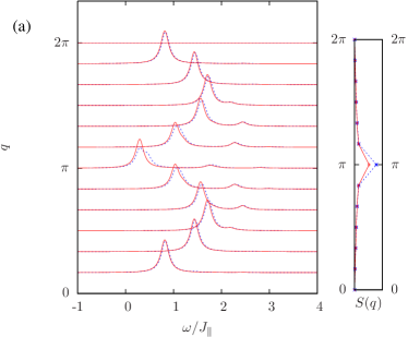
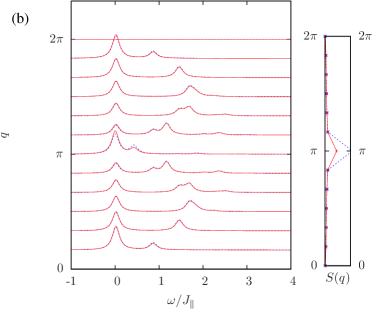
Figure 2: (Color online) Dynamical spin susceptibility in the weak coupling limit at $J_{\bot}/J_{\|}=0.1$: (a) ladder system ($\theta=0$); (b) single-pole ladder system $(\theta=\pi$). In both cases, results are obtained on $2\times 12$ lattices with ED techniques. We choose a broadening $s=0.1J_{\|}$. The red (solid) lines represent the bonding spectrum, $S(q,\omega)$, the blue (dashed) lines corresponds to the anti-bonding spectrum, $R(q,\omega)$. The spectral functions in the left panels are normalized to the structure factors $S(q,t=0),R(q,t=0)$, respectively; the latter are shown in the right panels.

Fig. 2 presents the spin excitation spectrum for the isotropic ladder $(\theta=0)$ and the single-pole ladder model ($\theta=\pi$) in the weak coupling region. Precisely, it shows the dynamical spin structure factor (depending on the momentum $q$ along the ladder), separately for the bonding ($S(q,\omega)$) and anti-bonding ($R(q,\omega)$) configuration. For the ladder, the dynamical spin structure factor for both bonding and anti-bonding cases displays features of the two spinons continuum of a single spin-$1/2$ chain des Cloizeaux and Pearson (1962).

Below we show, that such a continuum is qualitatively well reproduced by a mean-field theory, and corresponds to the particle-hole continuum stemming from the effective fermionic Hamiltonian. The continuum for bonding combination, $S(q,\omega)$, is characterized by a slightly lower energy due to the weak ferromagnetic coupling between the chains.

As apparent from Fig 2b, a narrow band emerges for the single-pole ladder model. We define its width, $W$, as the differences in energy between the low energy maxima at $q=\pi$ and $q=\pi/2$ in the spin excitation spectrum for $\theta=\pi$. Associating this band with the SN splitting of dangling spins, we expect the width, $W$, to scale as $J^{2}_{\perp}/J_{\|}$ in the weak coupling region. This is indeed confirmed for small system size in Fig. 3 where the ED data is found to fit well to a $W\propto J^{2}_{\perp}$ form.

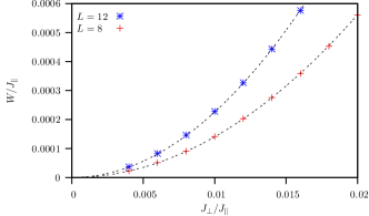
Figure 3: (Color online) ED results for the width $W$ in the single-pole ladder model ($\theta=\pi$). The effective SN interaction yields a bandwidth proportional to $J^{2}_{\perp}/J_{\|}$.

For reasons that will be clarified below, we also investigated the zero temperature spectral functions $S_{11}(q,\omega)$ and $S_{22}(q,\omega)$, Eq.  (5), with the emphasis on the weight, or residue, of the lowest excitation energy. This weight is a measure of the overlap between $\hat{S}^{z}_{l}(q)|0\rangle$ and the first low lying excitation as modeled with the effective Hamiltonian of Eq. (8). Fig. 4 plots this quantity, normalized by $\int_{0}^{\infty}{\rm d}\omega S_{ll}(q,\omega)$, that is:

$$Z_{l}(q)=\frac{|\langle 1|\hat{S}^{z}_{l}(q)|0\rangle|^{2}}{\langle S^{z}_{l}(-q)S^{z}_{l}(q)\rangle},$$ (25)

where the state $|1\rangle$ corresponds to the first magnetic excitation at wave number $q$. As apparent from the ED results for the single-pole ladder model (see Fig. 4), $Z_{2}(q=\pi)$ corresponding to the second leg is almost independent of $J_{\perp}$. Similar results are found for other momenta. It means that nearly all the spectral weight for spins in the second leg belongs to the well -defined lowest-lying excitation. This should be contrasted with the situation of spins the first leg, where only a fraction of the spectral weight belongs to this model, the rest participating the spin-wave continuum. Clearly, the continuum fraction in $S_{11}(q,\omega)$ should increase as $J_{\perp}$ is decreased up to the decoupled situation $J_{\perp}=0$, where one expects $Z_{2}(q=\pi)=0$.

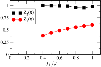
Figure 4: (Color online) Normalized residue as a function of $J_{\perp}/J_{\|}$ for the ferromagnetic single-pole ladder. The calculations were carried out with ED on an $2\times 8$ lattice.

We have also computed the spin gap $\Delta$ as a function of the interleg coupling $J_{\perp}$ for different values of $\theta$. Unfortunately, the finite size scaling becomes difficult in the weak coupling limit for all $\theta$ (data not shown) and an extrapolation to the thermodynamic limit is not feasible. We can only confirm the differences in the scaling behavior of the spin gap between the the single-pole model and the ladder model, where it is widely accepted that the gap opens linearly with the coupling between chains  Shelton et al. (1996); Larochelle and Greven (2004).

Concluding this subsection, we notice that the advantage of the ED method is its high accuracy, but the method is limited to relatively small system sizes. For the single pole ladder, when the gap becomes small and comparable to interlevel spacing $\sim J_{\|}/L$, the accuracy of the calculation becomes irrelevant.

IV.2 Quantum Monte Carlo, spin correlations

To extend our analysis to larger system sizes, we also used quantum Monte Carlo (QMC) methods, performing simulations at finite inverse temperature $\beta=1/T$. We applied two variants of the loop algorithm. For the spin-spin correlation function and for the string order parameter, discussed below, we used a discrete time algorithm. Evertz (2003) From the spin-spin correlation function we can then extract the spectral function via stochastic analytical continuation schemes. Sandvik (1998); Beach et al. (2004) In the next subsection, we also use a continuous time loop algorithm to directly compute the spin gap.

We start our QMC analysis with a discussion of the dynamical spin-spin correlations, which can be computed on much larger sizes than with ED. However, the energy resolution is limited and hence we can only use this approach at larger couplings than the ones reached with ED.

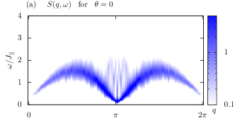
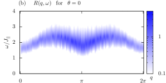
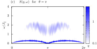
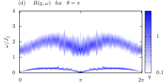
Figure 5: (Color online) QMC results of the bonding and antibonding dynamical spin susceptibility for the ladder ($\theta=0$) (two top panels) and single-pole ladder ($\theta=\pi$) (two bottom panels) systems at $J_{\bot}/J_{\|}=1.0$. $\beta J_{\|}=200$ was taken in the simulations.

The QMC results of the dynamical spin susceptibility for $\theta=0$ (ladder) and $\theta=\pi$ (single-pole ladder) with $2\times 100$ sites at $J_{\bot}/J_{\|}=1.0$ ($\beta J_{\|}=200$) are shown in Fig. 5 (these results were partly shown in Fig. 4 of Ref. Brünger et al. (2008)). At $\theta=0$, inversion symmetry ${\mathbf{S}}_{1,i}\leftrightarrow{\mathbf{S}}_{2,i}$ is present, such that the bonding and antibonding combinations do not mix. Since ${\mathbf{S}}_{i}$ is even under inversion symmetry (with respect to the transverse direction), $S(q,\omega)$ picks up the dynamics of the triplet excitations across the rungs. For ferromagnetic rung couplings $J_{\bot}>0$, the low energy spin dynamics of the model is apparent in $S(q,\omega)$ which in the strong coupling limit maps onto the spin structure factor of the Haldane chain. In contrast, ${\mathbf{R}}_{i}$ is odd under inversion symmetry and picks up the singlet excitations across the rungs. As apparent from Fig. 5b those excitations are located at a higher energy scale set by $J_{\bot}$ in the strong coupling limit. For the single-pole ladder model, $\theta=\pi$, a mixing of the bonding and anti-bonding sectors occurs. As apparent in Fig. 5c,d both $R(q,\omega)$ and $S(q,\omega)$ show high and low energy features. The low energy, narrow, dispersion curve in Fig. 5c is a consequence of the SN interaction and reflects the slow dynamics of triplets formed across the rungs.

In spite of the limited energy resolution of the QMC method, we can extract the value of the spin gap, by studying the spin correlation functions at long distances. Such analysis also provides an insight of the intermediate energy scales. We show the behavior of the correlations $\langle{S}^{z}_{1,i}{S}^{z}_{1,j}\rangle$ and $\langle{S}^{z}_{2,i}{S}^{z}_{2,j}\rangle$ as function of $|i-j|$ in Fig.  6 for a particular value $J_{\perp}=0.5J_{\|}$ ; the distance is measured in lattice spacings. We notice that beyond a certain length scale both correlation functions behave similarly, differing only in overall factor. We hence plot in Fig.  6 the function $\langle{S}^{z}_{1,i}{S}^{z}_{1,j}\rangle$ as is, while $\langle{S}^{z}_{2,i}{S}^{z}_{2,j}\rangle$ is multiplied by a factor discussed below; after this “normalization” both curves are indistinguishable at large distances $d\gtrsim 10$ (these results were partly shown in Fig. 3 of Ref. Brünger et al. (2008)). This indicates that the lowest-energy dynamics of dangling spins ${S}^{z}_{2,i}$ and of the main leg ${S}^{z}_{1,i}$ is the same slow dynamics of rung triplets, wherein these spins enter with different weight.

At largest distances an exponential decrease of correlations is observed, corresponding to a gap in the spectral weight of $S_{jj}(q,\omega)$. In the previous section we developed a theory which accounts in a semi-quantitative way the whole body of numerical findings. According to this theory, the long distance behavior of the spin-spin correlations is given by

$$|\langle{S}^{z}_{j,r}{S}^{z}_{j,0}\rangle|=\frac{w^{2}_{j}}{\pi}K_{0}\left(\frac{\Delta r}{v}\right).$$ (26)

with $K_{0}$ the modified Bessel function, $v\sim J_{\|}$ velocity of spin excitations, $w_{j}$ (with $j=1,2$) is the weight of the spin ${S}^{z}_{j,r}$ in the effective spin-1 variable of the single-pole ladder. As explained above, we expect $w_{j}\sim J_{\perp}/J_{\|}$ while $\Delta\sim J_{\perp}\exp(-J_{\|}/J_{\perp})$.

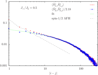
Figure 6: (Color online) Equal time spin-spin correlation function at $J_{\perp}/J_{\|}=0.5$ for the single-pole ladder along both chains. Simulations were done at $\beta J_{\|}=5000$ on a $2\times 800$ lattice.

In Fig. 6 we fit the long-ranged equal time spin-spin correlation function at $J_{\perp}/J_{\|}=0.5$ to this form. Several comments are in order.

a) Normalizing the spin-spin correlations of the dangling spin by a factor $2.18=w^{2}_{2}/w^{2}_{1}$ provides a perfect agreement between the long range correlations on both legs. Note that the numerical factor $2.18$ is close to $Z_{2}(q=\pi)/Z_{1}(q=\pi)\simeq 2.25$ as obtained from the data of Fig. 4. Hence the low energy dynamics of the spins on both legs are locked in together. This observation confirms the picture that the low lying spin mode observed in Fig. 5c indeed corresponds to the dynamics of triplets across the rungs.
b) One can read off a length scale at which the functional form of both correlation functions differs. This length scale marks the crossover from high to low energy beyond which an effective low energy theory can be applied.
c) In our previous paper Brünger et al. (2008) we also pointed out the existence of the intermediate asymptotic, $|i-j|^{-1/3}$, in case $J_{\perp}=0.3J_{\|}$. The existence of such power-law decay is interesting on its own, but the detailed description of this regime is beyond the scope of this study. This is the case when the gap becomes comparable to the energy spacing due to the finite size of the system, and it causes difficulties in other complementary numerical techniques, see e.g. DMRG results below.
d) For comparison we have plotted the spin-spin correlations of the spin-1/2 chain Affleck (1998); Essler et al. (2007) which, on a length scale set by the correlation length, decay much faster than the correlations of the single-pole ladder. This very slow decay should be seen as a direct consequence of the long ranged nature of the SN interaction.
e) The fit to the form of Eq. (26) is next to perfect thereby providing an excellent description of the low energy physics. The ratio of the gap to the velocity as well as the weight of the spins in effective spin-1 variable are plotted in Fig. 7. In particular, assuming a linear dependence of the weight (see below), we obtain $w^{2}_{2}=0.13J_{\perp}/J_{\|}$ and $w^{2}_{1}=0.060J_{\perp}/J_{\|}$. The gap values are fitted by an exponential law, $\Delta\sim J_{\perp}\exp(-J_{\|}/J_{\perp})$, as discussed in Sec.  III.1. In the next subsection, we will see that this exponential form provides an excellent fit to the spin gap directly measured in QMC. The parameters of the fit shown by a dashed line in Fig. 7 are explained in the last paragraph of the next subsection.

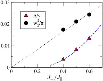
Figure 7: (Color online) Scales in the correlation function (26) on the second leg as a function of $J_{\perp}/J_{\|}$. The dotted line is a fit to a linear law and the dashed curve is a fit with $v=0.28J_{\|}$. The form of $\Delta$ is discussed at the end of Sec.  IV.3.

IV.3 Quantum Monte Carlo, spin gap

For the spin gap calculation the continuous-time loop algorithm of ALPS Alet et al. (2005) was used. Here, we can calculate the correlation length in imaginary time $\xi_{\tau}({q})$ for a given wave vector ${q}$ via a second moment estimator Cooper et al. (1982); Todo and Kato (2001):

$$\xi_{\tau}({q})=\frac{\beta}{2\pi}\left(\frac{\chi({q},\omega=0)}{\chi({q},\omega=2\pi/\beta)}-1\right)^{1/2}$$ (27)

with $\chi({q},\omega)=\int^{\beta}_{0}d\tau e^{i\omega\tau}\chi({q},\tau)$ the Fourier-transform of the imaginary time dynamical structure factor (7).

The inverse of $\xi_{\tau}({q})$ converges in the limit $L,\beta\rightarrow\infty$ to $\Delta({q})=E_{1}({{q}})-E_{0}$, if $\Delta({q})\neq 0$. Here $E_{1}({{q}})$ is the minimum of the dispersion at wave vector ${q}$ and $E_{0}$ the ground-state energy: the spin gap is simply obtained as $\Delta=\min_{{q}}\Delta({q})$. If the system is gapless at ${q}$, $\xi_{\tau}({q})^{-1}$ is an upper bound of the finite-size gap at ${q}$ for any finite $L$ and $\beta$. The full dispersion curve can therefore be calculated in principle with this method. In practice however, the simulations suffer from large statistical errors in $\chi({q},\omega)$ when ${q}$ is different from the wave vector of the lowest lying excitation. The situation can be ameliorated by using improved estimators Baker and Kawashima (1995) for the imaginary time dynamical structure factor, which is simply related to the loop sizes in the algorithm. The wave vector picked by the loops in the algorithm corresponds to the one given by the sign of the coupling constants Evertz (2003), which is in our case ${q}=(\pi,0)$ (for ferromagnetic $J_{\bot}>0$ and antiferromagnetic $J_{\|}<0$). The improved estimators have a smaller variance than conventional ones, and we therefore obtain good statistics for $\xi_{\tau}(\pi,0)$ and the spin gap $\Delta=\Delta(\pi,0)$ when it is finite.

Now we turn our attention to the spin gap as a function of the coupling $J_{\perp}$ and twist angle $\theta$ (see Fig. 8a) (these results were partly shown in Fig. 2 of Ref. Brünger et al. (2008)).

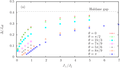
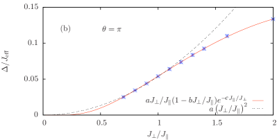
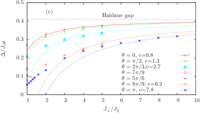
Figure 8: (Color online) (a) Size and temperature converged values of the spin gap $\Delta$ as a function of the coupling $J_{\perp}/J_{\|}$ for various twist angles. The gap is rescaled by $J_{\mathrm{eff}}=\tfrac{J_{\|}}{4}\left(1+\cos^{2}(\theta/2)\right)$ such that in the large-$J_{\perp}$-limit it converges asymptotically toward the Haldane gap of a AF spin-$1$ chain $\Delta_{H}/J_{\mathrm{eff}}\simeq 0.41$. (b) Spin gap for the single-pole ladder model, $\theta=\pi$. Lines denote quadratic and exponential fits for the spin gap (see text). (c) Spin-gap for SSHL at larger $J_{\perp}$ for different $\theta$s, see detailed discussion in Sec.  III.2.

In the strong coupling limit $J_{\perp}/J_{\|}\to\infty$ the model maps onto the AF spin-$1$ Heisenberg chain, Eq. (8) and we expect the Haldane gap $\Delta_{H}\simeq 0.41J_{\mathrm{eff}}$. This behavior is clearly apparent in Fig. 8a. However, as $\theta$ grows from $\theta=0$ to $\theta=\pi$ the approach to the Haldane limit becomes slower. Whereas the scaling for $\theta=0$ and $\theta=\pi/2$ are nearly similar, the scaling behavior for the single-pole ladder ($\theta=\pi$) differs, as can be seen in Fig.  8c. In Section III.2 we argued that at largest $J_{\perp}$ the gap should follow the law $\Delta\simeq 0.41J_{\mathrm{eff}}(1-c(\theta)J_{\mathrm{eff}}/{|J_{\perp}|})$. Now we confirm this picture by fitting the numerical data with this form at the largest $J_{\perp}$, as shown in Fig. 8c. We see that $c(\theta)$ definitely grows as a function of $\theta$ and reaches a large value $c(\theta)\simeq 8$ for the extreme case of the single-pole ladder, $\theta=\pi$. In the intermediate region, $1\lesssim J_{\perp}/J_{\|}\lesssim c(\theta)$, we cannot expect a good fit of the gap, as clearly visible in Fig. 8c.

For the ladder system ($\theta=0$) our data stand in agreement with the independent QMC calculations of Ref. Larochelle and Greven, 2004; the spin gap opens linearly with respect to the coupling $J_{\perp}$ up to logarithmic corrections. It is beyond the scope of this work to pin down the exact form of the logarithmic corrections, and we refer the reader to Ref. Larochelle and Greven, 2004 for further discussions. This behavior is stable up to to large twist angles, and it is only in the very close vicinity of $\theta=\pi$ that a different behavior is observed.

As discussed in the previous section, the spin gap at $\theta=\pi$ is expected to decrease exponentially with decreasing values of $J_{\perp}$, as $\propto J_{\perp}\exp(-J_{\|}/J_{\perp})$. In order to fit the QMC data of Fig. 8b in a wider region, $J_{\perp}\lesssim J_{\|}$, we also allow for a correction in the prefactor in this law, namely we assume the dependence $\Delta=aJ_{\perp}(1-bJ_{\perp}/J_{\|})\exp(-cJ_{\|}/J_{\perp})$. Fitting the data of Fig. 8b to this form gives $a=0.077,b=0.32,c=1.34$. These parameters can now be used to fit the data for the gap, $\Delta/v$, as extracted from the spatial decay of correlations in Fig.  7. The only adjustable parameter there is $v/J_{\|}$, and we obtain a good agreement in Fig. 7 for $v=0.28J_{\|}$. The effective model of the previous section leads to an expression $v=4w^{2}_{1}\xi J_{\|}$. Comparing these values, we determine the crossover scale $\xi=1.2J_{\|}/J_{\perp}$, which separates the long-distance behavior from the short-distance one. For the particular value $J_{\perp}=0.5J_{\|}$, we obtain $\xi\sim 3$, and this scale is clearly visible in the merging of curves for the spatial dependence of correlations in the first and second legs, as shown in Fig. 6. We further show in Fig. 8b the result of a quadratic fit to the gap $\Delta\sim(J_{\perp}/J_{\|})^{2}$. While such a fit is reasonable for low $J_{\perp}$ as remarked in Ref.  Brünger et al., 2008, the above exponential form appears to provide a better fit in a larger $J_{\perp}$ window.

IV.4 String Order Parameter

To pin down the nature of the ground state, and in particular for the single-pole ladder, we compute the string order parameter characterizing the Haldane phase. In the strong coupling region the system maps onto an effective spin-$1$ chain, for all twist angles $\theta$ and the ground state can viewed in terms a valence bond solid (VBS) Affleck et al. (1987); Affleck and Marston (1988); Schollwöck et al. (1996). In the VBS state the spins on a rung form triplets in such a way that neglecting triplets with z-component of spin $m=0$ reveals a Néel order. This hidden AF order, is characteristic of the Haldane phase and, as shown by Nijs and Rommelse den Nijs and Rommelse (1989), is revealed by the non-local string order parameter

$$\mathcal{O}_{s}=\Big{\langle}{S}^{z}_{n_{0}}\exp\left[i\pi\sum^{n_{0}+L/2-1}_{j=n_{0}}{S}^{z}_{j}\right]{S}^{z}_{n_{0}+L/2}\Big{\rangle}$$ (28)

where ${S}^{z}_{i}={S}^{z}_{1,i}+{S}^{z}_{2,i}$, $n_{0}$ stands for an arbitrary rung and $L$ denotes the system length. $\mathcal{O}_{s}$ is also sensitive to a true AF order. To distinguish between a hidden AF order and a true Néel order another order parameter has to be introduced den Nijs and Rommelse (1989)

$$\mathcal{O}_{H}=\Big{\langle}\exp\left[i\pi\sum^{n_{0}+L/2}_{j=n_{0}}{S}^{z}_{j}\right]\Big{\rangle}$$ (29)

which is zero in the Haldane phase (hidden AF order) and finite in the Néel phase. Starting from the strong coupling region where the system is clearly in the Haldane phase, $\mathcal{O}_{s}\neq 0$ and $\mathcal{O}_{H}=0$, we analyze the evolution of the string order parameter as a function of the coupling $J_{\perp}$ and the twist angle $\theta$. For $\theta=0$ the order parameter $\mathcal{O}_{s}$ stays finite and $\mathcal{O}_{H}$ is zero for all couplings. Hence the ladder system remains in the Haldane phase, independent of $J_{\perp}$.

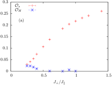
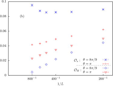
Figure 9: (Color online) (a) String order parameters $\mathcal{O}_{s}$ and $\mathcal{O}_{H}$ as a function of interleg coupling $J_{\perp}$ for $\theta=\pi$. In the parameter range $J_{\perp}/J_{\|}<0.5$ finite size effects are still present. (b) Finite size scaling of the order parameters for $\theta=8\pi/9$ ($J_{\perp}/J_{\|}=0.2$) and $\theta=\pi$ ($J_{\perp}/J_{\|}=0.3$). The simulations are carried out up to $\beta J_{\|}=7000$ and $2\times 800$ spins.

The situation for the single-pole ladder is much more delicate (see Fig. 9a, these results were shown in Fig. 5 of Ref. Brünger et al. (2008)). For $J_{\perp}/J_{\|}<0.4$ the string order parameter $\mathcal{O}_{H}$ appears to be non-zero, thus indicating Néel order. In the previous section we have shown, that at weak couplings and for $\theta=\pi$ the SN interaction generates a very slow decay of the spin correlations. For instance, the correlation length $\xi$ for $J_{\perp}/J_{\|}=0.3$ is larger than the system size and the very slow decay of the spin-spin correlation functions at distances smaller than $\xi$ mimics AF order. However, when increasing system size, one expects $\mathcal{O}_{H}$ to vanish and $\mathcal{O}_{s}$ to converge to a finite value. This expectation is supported by a finite size scaling of the string order parameters, as shown in Fig. 9b for $\theta=8\pi/9$ and $\theta=\pi$. The crossover between the AF order for small systems and the disordered phase is rather obvious for $\theta=8\pi/9$ ($\cos^{2}\tfrac{\theta}{2}\simeq 0.03$) at $J_{\perp}/J_{\|}=0.2$. For small lattice sizes the system seems to be in the AF ordered phase as indicated by the fact that both string order parameters are finite. However, for increasing lattice sizes the order $\mathcal{O}_{s}$ remains nearly constant, whereas the order parameter $\mathcal{O}_{H}$ decreases and finally vanishes. At this point the order parameter $\mathcal{O}_{s}$ increases again. For the single-pole ladder ($\theta=\pi$) at $J_{\perp}/J_{\|}=0.3$ we do not observe the disappearance of $\mathcal{O}_{H}$, which shows that finite size effects are strong in this case even for a system as large as $L=800$.

IV.5 DMRG analysis

In this section we present our analysis of the Hamiltonian, Eq. (1), with the use of the Density Matrix Renormalization Group (DMRG) White (1992) for the single-pole ladder, i.e.  $\theta=\pi$. Overall, our results presented in Fig. 10 clearly support a non-analytic exponential scaling of the gap in $J_{\perp}$ as suggested by the analytical considerations in this paper.

For the calculation of the spin gap the specific choice of the boundary condition (BC) is crucial. While DMRG prefers open BCs for numerical stability and accuracy, they must be dealt with carefully in order to separate boundary effects from bulk effects. Periodic boundary conditions can be applied within DMRG, Verstraete et al. (2004); Pippan et al. (2010) yet with somewhat limited accuracy and efficiency. In this paper we therefore adhere to the conventional DMRG with open BC. In order to still deal with a Hamiltonian with periodic BC, a long bond connecting the ends of the chain can be introduced for short system sizes. Alternatively for somewhat longer system sizes, the chain with periodic boundary can be reshaped into a double chain with ends connected to form a loop. We adopted the latter approach since it is stable in finding the ground state of the system. Nevertheless it is enormously costly numerically, and keeping up to 5120 states for chain lengths up to $L=256$ rungs total, the DMRG results still showed significant uncertainties in the ground state energy for small $J_{\perp}/J_{\|}$ insufficient to accurately resolve the exponentially small gap (see Fig. 10, panel a).

When compared to the other calculations (see, e.g., panel (d) below), the gap for periodic BC is consistently overestimated for small $J_{\perp}/J_{\|}$. This comes from the fact that the ground state is typically well-represented (smaller block entropy due to gap), while the excited state at larger $S_{z}^{\mathrm{tot}}$ has a larger block entropy as it is a part of the continuum. Due to the limited number of states kept, the excited state is less accurately represented which leads to an overestimated gap. This effect is more pronounced for large system sizes as can be clearly also seen from Fig. 10a.

At the same time the numerical data for the gap for large $J_{\perp}/J_{\|}$ are reliable, allowing for an extrapolation towards the known value of the Haldane gap with less than 1% relative error as shown in panel (a). The fitting-range used was $J_{\|}/J_{\perp}\leq 0.55$ as indicated by the vertical dotted guide in the panel. With a fit of the form $\Delta(J_{\perp})\sim e^{-\mathrm{const}\,J_{\|}/J_{\perp}}$ this shows that the Haldane gap is reached rather slowly when increasing $J_{\perp}$.

With periodic BC being of limited accuracy as explained above, we adopted the plain open BC also on the level of the Hamiltonian for the rest of the DMRG calculations. Hence we deal with a single ladder, in contrast to the connected double ladder above. Keeping up to 2560 states leads to clearly converged numerical data for all $J_{\perp}/J_{\|}$ analyzed. Note nevertheless, that the block entropy rises rapidly for $J_{\perp}/J_{\|}<0.5$ due to the near degeneracy of the dangling spins on the single-pole ladder in the limit $J_{\perp}/J_{\|}\rightarrow 0$.

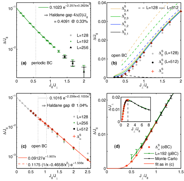
Figure 10: (Color online) DMRG analysis of the single-pole ladder ($\theta=\pi$) – Panel (a) shows the spin gap between the ground states of the $S_{z}=0$ and $S_{z}=1$ spin sectors for several system sizes using periodic BCs (double chain, see text). The error bars indicate the convergence with respect to the number of states $D$ kept (with an extrapolation in $1/D\rightarrow 0$ with $D\leq 5120$). The convergence to the Haldane gap for $J_{\perp}\gg J_{\|}$ is reproduced within 1% relative error, within the fitting-range at small $J_{\|}/J_{\perp}$ indicated by the vertical dotted line. Panel (b) shows spin gap data using open BCs for the ground states of several spin sectors $S_{z}\in\{0,1,2,3,4\}$. Keeping up to 2560 states, all energies are converged with negligible uncertainties. The consecutive energy differences (spin gap) $\Delta^{S}_{S_{z},S_{z}+1}$ between the ground states of the spin sectors $S_{z}$ and $S_{z}+1$ are plotted vs. $J_{\perp}/J_{\|}$ for $L=128$ (dashed) and $L=512$ (solid), respectively. The vertical order (top to bottom) of the entries in the legend matches the order of the lines appearing in the panel (top to bottom). The extrapolated spin gap $\Delta^{S}_{0}$ (grey and black dots for $L=128$ and $L=512$, respectively), as well as $\Delta^{S}_{\infty}$ (red crosses), as obtained from a finite size scaling of $\Delta^{S}_{1,2}$ for systems of length $L\in\{128,256,512\}$, are shown. Panel (c) shows $\Delta^{S}_{0}$ from panel (b) for $L\in\{128,512\}$ and also for $L=256$ together with $\Delta^{S}_{\infty}$ (all for open BC) on a semilog plot again with inverted x-axis similar to panel (a). The extrapolated value of the gap for small $J_{\|}/J_{\perp}$ for open BC compares well with the exact Haldane gap within 1% relative error already for the smaller system size $L=128$ (fit range up to first vertical dotted guide). Fits to the data for large $J_{\|}/J_{\perp}$ are shown in red solid and dashed curves. The fit range chosen is again indicated by the two vertical dotted guides, here for $J_{\|}/J_{\perp}>1$. Panel (d) summarizes the data obtained with periodic (green solid) and open (red asterisk) boundary conditions DMRG calculations, as compared with QMC data (black solid). The red solid line is a fit for large $J_{\|}/J_{\perp}$ similar to the one in panel (c). Error-bars indicate the respective uncertainty in energy. Inset shows that $\Delta/J_{\perp}$ reaches the maximum at $J_{\perp}\simeq 2J_{\|}$.

From the numerical analysis for systems with open BC, one observes spin 1/2 edge excitations visible in terms of an alternating finite $\langle S_{z,i}\rangle$ along the sites $i$ which decay exponentially with the distance from the ends of the chain. Kennedy (1990) As the total spin $S_{z}^{\mathrm{tot}}$ is a conserved quantum number, the individual symmetry sectors can be analyzed separately, with the overall ground state lying within $S_{z}^{\mathrm{tot}}=0$. However, as it turns out, the $S_{z}^{\mathrm{tot}}=0$ sector has clear $S_{z}=\pm\frac{1}{2}$ edge excitations with opposite signs being consistent with $S_{z}^{\mathrm{tot}}=0$. The situation is similar in the $S_{z}^{\mathrm{tot}}=1$ sector, but this time yet with equal signs of alternation, consistently adding up to $S_{z}^{\mathrm{tot}}=1$. Therefore $S_{z}^{\mathrm{tot}}=0$ and $S_{z}^{\mathrm{tot}}=1$ are degenerate in the thermodynamic limit yielding a four-fold degenerate ground-state due to the presence of the open boundary Kennedy (1990). Only starting with $S_{z}^{\mathrm{tot}}=2$ a true bulk excitation is generated. Almeida et al. (2007). In order to extract the spin gap, we therefore prefer to monitor the splitting in energy with respect to $S_{z}^{\mathrm{tot}}\geq 2$. To this end the energy differences $\Delta^{S}_{S_{z},S_{z}+1}$ between the ground states of the consecutive spin sectors $S_{z}$ and $S_{z}+1$ are calculated and plotted in Fig. 10b. From the above argument, $\Delta^{S}_{0,1}$ clearly vanishes in the thermodynamic limit as the overlap between the spin 1/2 excitations confined to the boundaries decays exponentially with system size. Therefore only $\Delta^{S}_{S_{z},S_{z}+1}$ for $S_{z}>0$ resembles the gap with a finite-size effect added with each increment of $S_{z}$. Note in Fig. 10b that all curves for $S_{z}>0$ start falling onto the same line as $L$ increases. This indicates, consistently with the notion of a spin gap, that for large enough system sizes each increment of $S_{z}^{\mathrm{tot}}$ by 1 costs an energy equal to the gap value. Note, however, that the lowest energy states for the $S_{z}>1$ sectors may already lie within a continuum of states.

The strategy then to extract the spin gap is two-fold: (i) extrapolation of $\Delta^{S}_{S_{z},S_{z}+1}$ for $S_{z}>0$ for constant system size $L$, using a quadratic fit towards $S_{z}=0$ to eliminate finite-size effects with increasing $S_{z}$,

$$\Delta^{S}_{0}\equiv\lim_{S_{z}\rightarrow 0}\Delta^{S}_{S_{z},S_{z}+1},\quad(L=\mathrm{const}),$$ (30)

(grey and black dots in Fig. 10b), and (ii) actual finite-size scaling on $\Delta^{S}_{1,2}$, i.e. the lowest $S_{z}$ that yields a finite spin gap $\Delta^{S}_{S_{z},S_{z}+1}$ in the thermodynamic limit,

$$\Delta^{S}_{\infty}\equiv\lim_{1/L\rightarrow 0}\Delta^{S}_{1,2}$$ (31)

(red crosses Fig. 10b). As can be seen in the same panel, both strategies nicely agree with each other for $L=512$, indicating that the data are well converged and consistent. It also shows that Eq. (30) is a valid way of extracting the spin gap for systems that are large enough.

In order to analyze the data at small $J_{\perp}/J_{\|}$, the data for $\Delta^{S}_{0}$ and $\Delta^{S}_{\infty}$ are (re)plotted in Fig. 10c with inverted x-axis on a semilog-y plot, as we expect a non-analytic behavior of the form $\Delta\sim e^{-\mathrm{const}\,J_{\|}/J_{\perp}}$ (and as motivated by previous studies on spin ladders too White and Affleck (1996)). As a consistency check for open BCs, the gap $\Delta^{S}_{0}$ for $L=128$ is again extrapolated towards $J_{\|}/J_{\perp}\rightarrow 0$ to retrieve the Haldane gap with reasonable accuracy of 1%.

For large $J_{\|}/J_{\perp}>1$, the gap $\Delta^{S}_{\infty}$ in the thermodynamic limit (red crosses in Fig. 10c) can be fitted nicely using exponential forms of either type

$$\Delta(J^{\prime}) = a_{0}e^{-{c_{1}}/{J^{\prime}}}\text{, and}$$ (32a)

$$\Delta(J^{\prime}) = \left(a_{1}J^{\prime}-a_{2}(J^{\prime})^{2}\right)e^{-{c_{2}}/{J^{\prime}}}$$ (32b)

with $J^{\prime}\equiv{J_{\perp}}/{J_{\|}}$, and $a_{i}$ and $c_{i}$ being fitting parameters (see Fig. 10c where $x\equiv 1/J^{\prime}$). Note that the $(J^{\prime})^{2}$ term in Eq. (32b) is important to obtain a clear agreement with the numerical data.The data are equally well fitted by both forms in the region $J_{\|}/J_{\perp}>1$, with deviations of the fit in Eq. (32b) (dashed line in Fig. 10c) visible only outside the fitted region, at $J_{\|}<J_{\perp}$. Note also that despite the fact that the fitting-range chosen to be $J_{\|}/J_{\perp}\in\ [1.05,2.25]$ (as indicated by the vertical dotted guides in Fig. 10c), both fits extrapolate well up the last data point at 2.5.

Finally, the DMRG results for the gap are summarized and directly compared to the QMC simulations in Fig. 10d, as a function of $J_{\perp}/J_{\|}$. The gap $\Delta^{S}_{\infty}$ in the thermodynamic limit (red asterisks) clearly lies within the error bars of the other less accurate data sets, while its own error bars are negligible. The results obtained this way are then reliable down to smaller $J_{\perp}/J_{\|}$. The exponential fit reproduced from Fig. 10c (solid red line) in panel (d), finally, illustrates the extremely fast decay of the gap towards small $J_{\perp}$. Yet as clearly supported by Fig. 10c, the spin gap remains finite in this region. The inset in Fig. 10d illustrates that, when scaled to $J_{\perp}$, the gap in the single-pole ladder has a maximum at $J_{\perp}\simeq 2J_{\|}$ and decreases exponentially at smaller $J_{\perp}$. This is to be contrasted with the symmetrical ladder where $\Delta/J_{\perp}$ saturates to a constant at $J_{\perp}\to 0$.

V Conclusions

In conclusion, we investigated asymmetric spin ladders, with different values of exchange interaction of spins $S=1/2$ along the two legs as parametrized by $\theta$. For ferromagnetic rung coupling $J_{\perp}$ the spectrum of excitations is characterized by a Haldane gap, as expected for the effective spin-1 rung variables which are coupled antiferromagnetically along the chains. We confirm this by the numerical analysis of the spin gap, spin correlation functions and of the corresponding string order parameter.

The most intriguing behavior is observed near the single-pole situation, i.e. in the absence of exchange along the second leg. Our extensive numerical analysis shows that the spin gap decreases with $J_{\perp}$ exponentially fast, $\Delta\sim J_{\perp}\exp(-J_{\|}/J_{\perp})$, unlike the conventional symmetric ladder behavior, $\Delta\sim J_{\perp}$. In order to explain the whole body of numerical data, we develop a theory, which takes into account the indirect Suhl-Nakamura interaction between spins and the formation of large effective blocks of spins. In a certain sense, the formula for the gap as obtained from this approach combines the “quantum” prefactor $J_{\perp}$ and the semi-classical exponent $\exp(-J_{\|}/J_{\perp})$ arising from the large-block picture.

In summary, we have a strong evidence that a spin gap opens for any $J_{\perp}$ but it may be exponentially suppressed nearly single-pole situation. This smallness leads to difficulties in the actual observation of this gap, both due to the finite resolution of the tool employed (numerical or experimental) and to the finite-size effects associated with a large correlation length.

The case of a negligible gap was reported in Ref. Brünger et al., 2008 for $J_{\perp}=0.3J_{\|}$. We did not discuss this situation in the present paper, since at these parameters the correlation length is larger than the system size and the true string order parameter is not formed, cf. Fig. 9. In such case the observed power-law decrease of correlation functions should be viewed as an intermediate asymptote, and the origin of the particular value of the decay exponent reported in Brünger et al. (2008) is not clear.

Appendix A Jordan-Wigner Mean-Field Approach

The definition of the Jordan-Wigner transformation for the ladder topology relies on the choice of a path labeling different sites. With the choice shown in Fig. 11a it reads:

$${S}^{z}_{1,i} = {n}_{1,i}-\tfrac{1}{2}\quad{S}^{z}_{2,i}={n}_{2,i}-\tfrac{1}{2}$$

$${S}^{+}_{1,i} = {c}^{\dagger}_{1,i}\exp\big{(}-\mathrm{i}\pi\sum^{i-1}_{l=1}({n}_{1,l}+{n}_{2,l})\big{)}$$

$${S}^{+}_{2,i} = {c}^{\dagger}_{2,i}\exp\big{(}-\mathrm{i}\pi(\sum^{i}_{l=1}{n}_{1,l}+\sum^{i-1}_{l=1}{n}_{2,l}\big{)})$$ (33)

where ${n}_{\alpha,i}={c}^{\dagger}_{\alpha,i}{c}_{\alpha,i}$ is the density operator at site $i$ with leg index $\alpha=1,2$. ${c}^{\dagger}_{\alpha,i}$ and ${c}_{\alpha,i}$ are spinless fermionic creation and annihilation operators which satisfy the anticommutation rules $\left\{{c}_{\alpha,i},{c}^{\dagger}_{\beta,j}\right\}=\delta_{ij}\delta_{\alpha\beta}.$

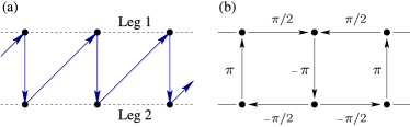
Figure 11: (Color online) (a) Zigzag path used for the Jordan-Wigner transformation, Eq.  (33), (b) gauge transformation, leading to Eq. (35).

Before proceeding to the details of the mean-field calculations below, let us summarize the results obtained within this approach. The ground state of the asymmetric ladder is characterized by spinless fermions circulating around a plaquette thereby allowing for a $\pi$-flux phase as solution of the mean-field equations. This leads to a spin gap $\Delta\propto|J_{\perp}|\cos(\theta/2)$ for $|J_{\perp}|\lesssim J_{\|}\cos(\theta/2)$. Such regime is unavailable for the single-pole system at $\theta=\pi$ in which case we obtain an (indirect) spin gap $\Delta\propto J_{\bot}^{2}/J_{\|}$. The mean-field also predicts a smooth crossover between these two regimes.

Our analysis is rather standard and similar to Ref. Azzouz et al., 1994. After application of the Jordan-Wigner transformation, the Heisenberg Hamiltonian of Eq. (1) can be written as:

$${\mathcal{H}} = -\frac{J_{\|}}{2}\sum^{L}_{i=1}\left((\hat{A}^{(1)}_{i})^{2}-\hat{A}^{(1)}_{i}e^{\mathrm{i}\pi\hat{n}_{i,2}}\right)$$

$$-\frac{J_{\|}}{2}\cos^{2}\left(\tfrac{\theta}{2}\right)\sum^{L}_{i=1}\left((\hat{A}^{(2)}_{i})^{2}-\hat{A}^{(2)}_{i}e^{\mathrm{i}\pi\hat{n}_{i+1,1}}\right),$$

$$+\frac{J_{\bot}}{2}\sum^{L}_{i=1}(\hat{B}_{i}^{2}-\hat{B}_{i})$$

Here, we have defined

$$\hat{A}^{(\alpha)}_{i}={c}^{\dagger}_{\alpha,i}{c}_{\alpha,i+1}+h.c.\,\,,\quad\hat{B}_{i}={c}^{\dagger}_{1,i}{c}_{2,i}+h.c.$$ (34)

We restrict ourselves below to a phase with zero magnetization, $\langle{S}^{z}_{\alpha,i}\rangle=0$, which corresponds to $\langle{n}_{\alpha,i}\rangle=\frac{1}{2}$. To proceed further we will replace ${n}_{\alpha,i}$ by its mean value. Although this simplification cannot be rigorously justified Aristov (1998) and more elaborate treatments are possible in a Jordan-Wigner approach Nunner and Kopp (2004), we show below that it qualitatively reproduces the results available by more sophisticated methods.

The replacement $e^{\mathrm{i}\pi\hat{n}_{\alpha,i+1}}\to i$ defines a spiral $U(1)$ phase shift for fermions on each leg. The relative phase between these spirals demarcate two qualitatively different situations. In one case the phase flux $\Phi$ through each plaquette is zero and in another case it is equal to $\pi$. Using the gauge transformation, we can reduce the $\Phi$-flux phase effective Hamiltonian to the form

$$\mathcal{H}_{\Phi}= -\frac{J_{\|}}{2}\sum_{l}\left((\hat{A}^{(1)}_{l})^{2}+\hat{A}^{(1)}_{l}\right)$$ (35)

$$-\frac{J_{\|}}{2}\cos^{2}\left(\tfrac{\theta}{2}\right)\sum_{l}\left((\hat{A}^{(2)}_{l})^{2}+\hat{A}^{(2)}_{l}\right),$$

$$+\frac{J_{\bot}}{2}\sum_{l}(\hat{B}_{l}^{2}+e^{i\Phi l}\hat{B}_{l})$$

with a checkerboard character of coupling in the $J_{\bot}$ channel happening in the $\pi$-flux case, $\Phi=\pi$. On the other hand, the $0$-flux case is characterized by a uniform $J_{\bot}$ coupling, $e^{i\Phi l}\to 1$ in Eq. (35) .

We then use the mean-field decoupling,

$$\langle\hat{A}^{(j)}_{l}\rangle=A^{(j)},\quad\langle\hat{B}_{l}\rangle=e^{i\Phi l}B$$

for the quadratic part of the Hamiltonian (35), where the special property $\hat{B}_{l}^{3}=\hat{B}_{l}$, $(\hat{A}^{(j)}_{l})^{3}=\hat{A}^{(j)}_{l}$ should be taken into account. The remaining Hamiltonian is quadratic in fermions and its spectrum is easily found. It can be shown that the $\pi$-flux phase provides a lower ground state energy, and hence we focus on this phase from now on. From the consistency equations below it can be shown that $A^{(1)}=A^{(2)}=A$, and we can use this observation to simplify our subsequent formulas.

The spectrum has two bands,

$$\varepsilon^{(\pm)}_{q} = \tfrac{1}{2}J_{\|}(1+A)\sin^{2}(\tfrac{\theta}{2})\cos q\pm\tfrac{1}{2}E_{q},$$ (36)

$$E_{q} = \sqrt{(J_{\|}(1+A)(1+\cos^{2}(\tfrac{\theta}{2}))\cos q)^{2}+J^{2}_{\perp}(1+B)^{2}},$$

and this dispersion should be combined with the consistency conditions

$$A = \frac{1}{L}\sum_{{q}}\frac{J_{\|}(1+A)(1+\cos^{2}(\tfrac{\theta}{2}))\cos^{2}q}{E_{q}},$$ (37)

$$B = \frac{1}{L}\sum_{{q}}\frac{J_{\bot}(1+B)}{2E_{q}},$$ (38)

where the thermodynamic limit $\frac{1}{L}\sum_{{q}}\to\int dq/2\pi$ is assumed.

In the limit $J_{\perp}\to 0$ we have $A\simeq 2/\pi$ and

$$B\simeq\frac{(J_{\perp}/J_{\|})\ln(J_{\|}/J_{\perp}c_{1})}{(1+\pi/2)(1+\cos^{2}(\tfrac{\theta}{2}))}.$$

with $c_{1}\sim 1$.

At half-filling, corresponding to a vanishing total magnetization in the spin language, a direct gap is given by $\varepsilon^{(+)}_{q}-\varepsilon^{(-)}_{q}=E_{q}$ at $q=\pi/2$ or

$$\Delta_{0}= \left|J_{\bot}\left(1+B\right)\right|,$$ (39)

$$\simeq \left|J_{\bot}\right|\left(1+O((J_{\perp}/J_{\|})\ln(J_{\|}/J_{\perp}))\right)$$

Hence, this simple mean-field approach is consistent (including logarithmic corrections) with bosonization Shelton et al. (1996) and quantum Monte Carlo simulations Larochelle and Greven (2004) for which a spin gap of the form Eq. (39) is found in the weak coupling limit.

The indirect gap, which is the minimum excitation energy in the spin system at zero temperature, is defined as $\Delta=\min_{q}\varepsilon^{(+)}_{q}-\max_{k}\varepsilon^{(-)}_{k}=2\min_{q}\varepsilon^{(+)}_{q}$. The qualitative form of the spectrum (36) at $\theta\simeq\pi$ is depicted in Fig. 2 of Ref.  Kiselev et al., 2005b. For small $J_{\bot}$, a flat band is apparent reflecting the macroscopic degeneracy of the model at $\theta=\pi$ and $J_{\bot}=0$. This leads to a dense spectrum of particle-hole excitations at low energies. A straightforward calculation shows that

$$\Delta=\Delta_{0}\frac{2\cos\tfrac{\theta}{2}}{1+\cos^{2}\tfrac{\theta}{2}}$$ (40)

at $\cos\tfrac{\theta}{2}\sim 1$ and small enough $J_{\perp}$. When $\cos\tfrac{\theta}{2}\to 0$, the domain of linear dependence of $\Delta$ on $J_{\perp}$ disappears and we have the quadratic law. Expressing energies in units of $\epsilon_{0}=J_{\|}(1+A)(1+\cos^{2}\tfrac{\theta}{2})$, we obtain for small $J_{\perp}/\epsilon_{0},\cos\tfrac{\theta}{2}\ll 1$ :

$$\Delta \simeq 2J_{\perp}\cos\tfrac{\theta}{2},\quad J_{\perp}<2\epsilon_{0}\cos\tfrac{\theta}{2}$$ (41)

$$\simeq J_{\perp}^{2}/(2\epsilon_{0})+2\epsilon_{0}\cos^{2}\tfrac{\theta}{2},\quad J_{\perp}>2\epsilon_{0}\cos\tfrac{\theta}{2}.$$

A linear regime for the indirect gap occurs for incommensurate $q$ in the above expression $\min_{q}\varepsilon^{(+)}_{q}$, whereas the quadratic regime in (41) corresponds to the difference $\varepsilon^{(+)}_{q=\pi}-\max_{k}\varepsilon^{(-)}_{k=0}$, i.e. commensurate wave-vector $\pi$ of the particle-hole excitation.

Appendix B magnons for long-range interaction

We use the Dyson-Maleyev representation of spin operators. In a predominantly AF situation, we write

$$S^{z}_{l}= (s-a_{l}^{\dagger}a_{l})(-1)^{l}$$ (42)

$$S^{x}_{l}= \sqrt{s/2}(a_{l}^{\dagger}+a_{l}-a^{\dagger}_{l}a_{l}^{2}/(2s))$$

$$S^{y}_{l}= i\sqrt{s/2}(a_{l}^{\dagger}-a_{l}+a^{\dagger}_{l}a_{l}^{2}/(2s))(-1)^{l}$$

For spins in different sublattices we have

$${\bf S}_{1}{\bf S}_{2} = -s^{2}-s+s(a^{\dagger}_{1}+a_{2})(a^{\dagger}_{2}+a_{1})+\ldots$$

and for spins in the same sublattice :

$${\bf S}_{1}{\bf S}_{3} = s^{2}-s(a^{\dagger}_{1}-a^{\dagger}_{3})(a_{1}-a_{3})+\ldots$$

Adopting the FM interaction $\tilde{V}(r)$ within one sublattice and AFM interaction $V(r)$ between sublattices, we come to the linearized Hamiltonian :

$$H=s\sum_{k}(2a^{\dagger}_{k}a_{k}[V(0)+\tilde{V}(0)-\tilde{V}(k)]+V(k)[a^{\dagger}_{k}a^{\dagger}_{-k}+h.c.])$$ (43)

Notice that we have $V(k+\pi)=-V(k)$ and $\tilde{V}(k+\pi)=\tilde{V}(k)$. To stress the similarity to acoustic phonons, the last equation can also be rewritten as

$$H=s\sum_{k}(g_{k+\pi}P_{k}P_{-k}+g_{k}Q_{k}Q_{-k})$$ (44)

where

$$P_{k}= (a^{\dagger}_{k}+a_{-k})/\sqrt{2}$$ (45)

$$Q_{k}= i(a^{\dagger}_{k}-a_{-k})/\sqrt{2}$$

$$g_{k}= [V(0)-V(k)+\tilde{V}(0)-\tilde{V}(k)]$$

so that canonical commutation relations hold, $[P_{k},Q_{q}]=i\delta(k+q)$. For $k\simeq 0$ we have $g_{k}\propto k^{2}$, $g_{k+\pi}\simeq 2V(0)$ the spectrum $\omega(k)=2s\sqrt{g_{k}g_{k+\pi}}\sim k$ is linear for small $k$. The analogy with acoustic phonons is incomplete, because in the second magnetic Brillouin zone (close to the point $k\simeq\pi$) the role of $P_{k}$ and $Q_{k}$ is reversed with respect to the form of their correlation functions.

For the dynamical susceptibility, $\chi^{xx}$, the representation in terms of $a$ is the same for both sublattices and we have $S^{x}_{k}=\sqrt{s}P_{k}$. The equations of motion read

$$\partial_{t}P_{k}= 2sg_{k}Q_{k}$$ (46)

$$\partial_{t}Q_{k}= -2sg_{k+\pi}P_{k}$$

and hence

$$\chi^{xx}(k,\omega)=s\frac{2sg_{k}}{\omega(k)^{2}-\omega^{2}}$$ (47)

For the nearest neighbor interaction $J$ this formula simplifies to:

$$S\frac{2SJ(1-\cos q)}{\Omega_{m}^{2}+(2SJ\sin q)^{2}}.$$ (48)

References

- Lee et al. (2002) S.-W. Lee, C. Mao, C. E. Flynn, and A. M. Belcher, Science 296, 892 (2002).
- Bloch et al. (2008) I. Bloch, J. Dalibard, and W. Zwerger, Rev. Mod. Phys. 80, 885 (2008).
- Giamarchi (2010) T. Giamarchi, in Understanding Quantum Phase Transitions, edited by L. D. Carr (CRC Press / Taylor & Francis, 2010), arXiv:1007.1029v1.
- Shelton et al. (1996) D. G. Shelton, A. A. Nersesyan, and A. M. Tsvelik, Phys. Rev. B 53, 8521 (1996).
- Schollwöck et al. (1996) U. Schollwöck, T. Jolicœur, and T. Garel, Phys. Rev. B 53, 3304 (1996).
- Gogolin et al. (1998) A. O. Gogolin, A. A. Nersesyan, and A. M. Tsvelik, Bosonization and Strongly Correlated Systems (Cambridge University Press, Cambridge, 1998).
- Giamarchi (2003) T. Giamarchi, Quantum Physics in One Dimension (Clarendon Press, Oxford, 2003).
- Affleck (1989) I. Affleck, Journal of Physics: Condensed Matter 1, 3047 (1989).
- Haldane (1983) F. D. M. Haldane, Phys. Rev. Lett. 50, 1153 (1983).
- Affleck and Lieb (1986) I. Affleck and E. H. Lieb, Lett. Math. Phys. 12, 57 (1986).
- Nightingale and Blöte (1986) M. P. Nightingale and H. W. J. Blöte, Phys. Rev. B 33, 659 (1986).
- Takahashi (1989) M. Takahashi, Phys. Rev. Lett. 62, 2313 (1989).
- White and Huse (1993) S. R. White and D. A. Huse, Phys. Rev. B 48, 3844 (1993).
- Deisz et al. (1993) J. Deisz, M. Jarrell, and D. L. Cox, Phys. Rev. B 48, 10227 (1993).
- Golinelli et al. (1994) O. Golinelli, T. Jolicoeur, and R. Lacaze, Phys. Rev. B 50, 3037 (1994).
- Todo and Kato (2001) S. Todo and K. Kato, Phys. Rev. Lett. 87, 047203 (2001).
- Honda et al. (1998) Z. Honda, H. Asakawa, and K. Katsumata, Phys. Rev. Lett. 81, 2566 (1998).
- Zheludev et al. (2003) A. Zheludev, Z. Honda, C. L. Broholm, K. Katsumata, S. M. Shapiro, A. Kolezhuk, S. Park, and Y. Qiu, Phys. Rev. B 68, 134438 (2003).
- Dagotto and Rice (1996) E. Dagotto and T. M. Rice, Science 271, 618 (1996).
- Kiselev et al. (2005a) M. N. Kiselev, D. N. Aristov, and K. Kikoin, Phys. Rev. B 71, 092404 (2005a).
- Kiselev et al. (2005b) M. N. Kiselev, D. N. Aristov, and K. Kikoin, Physica B 359-361, 1406 (2005b).
- Essler et al. (2007) F. H. L. Essler, T. Kuzmenko, and I. A. Zaliznyak, Phys. Rev. B 76, 115108 (2007).
- Brünger et al. (2008) C. Brünger, F. Assaad, S. Capponi, F. Alet, D. Aristov, and M. Kiselev, Phys. Rev. Lett. 100, 017202 (2008).
- Hosokoshi et al. (1999) Y. Hosokoshi, Y. Nakazawa, K. Inoue, K. Takizawa, H. Nakano, M. Takahashi, and T. Goto, Phys. Rev. B 60, 12924 (1999).
- Aristov et al. (2007) D. N. Aristov, M. N. Kiselev, and K. Kikoin, Phys. Rev. B 75, 224405 (2007).
- Suhl (1957) H. Suhl, Phys. Rev. 109, 606 (1957).
- Nakamura (1958) T. Nakamura, Progr. Theor. Phys. 20, 542 (1958).
- Aristov et al. (1994) D. N. Aristov, S. V. Maleyev, M. Guillaume, A. Furrer, and C. J. Carlile, Z. Phys. B 95, 291 (1994).
- Aristov (1997) D. N. Aristov, Phys. Rev. B 55, 8064 (1997).
- Affleck and Oshikawa (1999) I. Affleck and M. Oshikawa, Phys. Rev. B 60, 1038 (1999).
- Aristov and Kiselev (2004) D. N. Aristov and M. N. Kiselev, Phys. Rev. B 70, 224402 (2004).
- Huang (1987) K. Huang, Statistical mechanics (Wiley, New York, 1987).
- Lanczos (1950) C. Lanczos, J. Research Nat. Bureau Standards 45, 255 (1950).
- Dagotto (1994) E. Dagotto, Rev. Mod. .Phys. 66, 763 (1994).
- des Cloizeaux and Pearson (1962) J. des Cloizeaux and J. J. Pearson, Phys. Rev. 128, 2131 (1962).
- Larochelle and Greven (2004) S. Larochelle and M. Greven, Phys. Rev. B. 69, 092408 (2004).
- Evertz (2003) H. G. Evertz, Adv. in Phys. 52, 1 (2003).
- Sandvik (1998) A. Sandvik, Phys. Rev. B 57, 10287 (1998).
- Beach et al. (2004) K. S. D. Beach, P. A. Lee, and P. Monthoux, Phys. Rev. Lett. 92, 026401 (2004).
- Affleck (1998) I. Affleck, J. Phys. A: Math. Gen. 31, 4573 (1998).
- Alet et al. (2005) F. Alet, P. Dayal, A. Grzesik, A. Honecker, M. Körner, A. Läuchli, S. R. Manmana, I. P. McCulloch, F. Michel, R. M. Noack, et al., Jpn. J. Appl. Phys. 74, 30 (2005).
- Cooper et al. (1982) F. Cooper, B. Freedman, and D. Preston, Nucl. Phys. B 210, 210 (1982).
- Baker and Kawashima (1995) G. A. Baker and N. Kawashima, Phys. Rev. Lett. 75, 994 (1995).
- Affleck et al. (1987) I. Affleck, T. Kennedy, E. H. Lieb, and H. Tasaki, Phys. Rev. Letters 59, 799 (1987).
- Affleck and Marston (1988) I. Affleck and J. B. Marston, Phys. Rev. B 37, 3774 (1988).
- den Nijs and Rommelse (1989) M. den Nijs and K. Rommelse, Phys. Rev. B. 40, 4709 (1989).
- White (1992) S. R. White, Phys. Rev. Lett. 69, 2863 (1992).
- Verstraete et al. (2004) F. Verstraete, D. Porras, and J. I. Cirac, Phys. Rev. Lett. 93, 227205 (2004).
- Pippan et al. (2010) P. Pippan, S. R. White, and H. G. Evertz, Phys. Rev. B 81, 081103 (2010).
- Kennedy (1990) T. Kennedy, Journal of Physics: Condensed Matter 2, 5737 (1990).
- Almeida et al. (2007) J. Almeida, M. A. Martin-Delgado, and G. Sierra, Phys. Rev. B 76, 184428 (2007).
- White and Affleck (1996) S. R. White and I. Affleck, Phys. Rev. B 54, 9862 (1996).
- Azzouz et al. (1994) M. Azzouz, L. Chen, and S. Moukouri, Phys. Rev. B 50, 6233 (1994).
- Aristov (1998) D. N. Aristov, Phys. Rev. B 57, 12825 (1998).
- Nunner and Kopp (2004) T. S. Nunner and T. Kopp, Phys. Rev. B. 69, 104419 (2004).