Calculation of aggregate loss distributions

Abstract

Estimation of the operational risk capital under the Loss Distribution Approach requires evaluation of aggregate (compound) loss distributions which is one of the classic problems in risk theory. Closed-form solutions are not available for the distributions typically used in operational risk. However with modern computer processing power, these distributions can be calculated virtually exactly using numerical methods. This paper reviews numerical algorithms that can be successfully used to calculate the aggregate loss distributions. In particular Monte Carlo, Panjer recursion and Fourier transformation methods are presented and compared. Also, several closed-form approximations based on moment matching and asymptotic result for heavy-tailed distributions are reviewed.

Keywords: aggregate loss distribution, compound distribution, Monte Carlo, Panjer recursion, Fast Fourier Transform, loss distribution approach, operational risk.

This is a preprint of an article published in
The Journal of Operational Risk 5(2), pp. 3-40, 2010.
www.journalofoperationalrisk.com

1 Introduction and Model

Estimation of the operational risk capital under the Loss Distribution Approach (LDA) requires calculation of the distribution for the aggregate (compound) loss

$$Z=X_{1}+\cdots+X_{N},$$ (1)

where the frequency $N$ is a discrete random variable and $X_{1},\ldots,X_{N}$ are positive random severities. For a recent review of LDA, see Chernobai et al (2007) and Shevchenko (2010). This is one of the classical problems in risk theory. Closed-form solutions are not available for the distributions typically used in operational risk. However with modern computer processing power, these distributions can be calculated virtually exactly using numerical algorithms. The easiest to implement is the Monte Carlo method. However, because it is typically slow, Panjer recursion and Fourier inversion techniques are widely used. Both have a long history, but their applications to computing very high quantiles of the compound distribution functions with high frequencies and heavy tails are only recent developments and various pitfalls exist.

This paper presents review and tutorial on the methods used to calculate the distribution of the aggregate loss (1) over a chosen time period. The following model assumptions and notation are used:

• Only one risk cell and one time period are considered. Typically, the calculation of the aggregate loss over a one-year time period is required in operational risk.

• $N$ is the number of events over the time period (frequency) modelled as a discrete random variable with probability mass function $p_{k}=\Pr[N=k]$, $k=0,1,\ldots\;$. There is a finite probability of no loss occurring over the considered time period if $N=0$ is allowed, i.e. $\Pr[Z=0]=\Pr[N=0]$.

• $X_{i}$, $i\geq 1$ are positive severities of the events (loss amounts) modelled as independent and identically distributed random variables from a continuous distribution function $F(x)$ with $x\geq 0$ and $F(0)=0$. The corresponding density function is denoted as $f(x)$.

• $N$ and $X_{i}$ are independent for all $i$, i.e. the frequencies and severities are independent.

• The distribution and density functions of the aggregate loss $Z$ are denoted as $H(z)$ and $h(z)$ respectively.

• All model parameters (parameters of the frequency and severity distributions) are assumed to be known. In real application, the model parameters are unknown and estimated using past data. The impact of uncertainty in parameter estimates on the annual loss distribution can be significant for low-frequency/high-severity operational risks due to limited historical data (see Shevchenko (2008)); this topic is beyond the purpose of this paper.

In general, there are two types of analytic solutions for calculating the compound distribution $H(z)$. These are based on convolutions and method of characteristic functions described in Section 2. The moments of the compound loss can be derived in closed-form via the moments of frequency and severity; these are presented in Section 2 as well. Section 3 gives the analytic expressions for the Value-at-Risk and expected shortfall risk measures. Typically, the analytic solutions do not have closed-form and numerical methods such as Monte Carlo (MC), Panjer recursion, Fast Fourier Transform (FFT) or direct integration are required; these are described in Sections 4, 5, 6 and 7 respectively. Comparison of these methods is discussed in Section 8. Finally, Section 9 reviews several closed-form approximations. The distributions used throughout the paper are formally defined in Appendix.

2 Analytic Solutions

Analytic calculation of the compound distribution can be accomplished using methods of convolutions and characteristic functions. This section presents these methods and derives the moments of the compound distribution.

2.1 Solution via Convolutions

It is well-known that the density and distribution functions of the sum of two independent continuous random variables $Y_{1}\sim F_{1}(\cdot)$ and $Y_{2}\sim F_{2}(\cdot)$, with the densities $f_{1}(\cdot)$ and $f_{2}(\cdot)$ respectively, can be calculated via convolution as

$$f_{Y_{1}+Y_{2}}(y)=(f_{1}\ast f_{2})(y)=\int f_{2}(y-y_{1})f_{1}(y_{1})dy_{1}$$ (2)

and

$$F_{Y_{1}+Y_{2}}(y)=(F_{1}\ast F_{2})(y)=\int F_{2}(y-y_{1})f_{1}(y_{1})dy_{1}$$ (3)

respectively. Hereafter, notation $f_{1}\ast f_{2}$ denotes convolution of $f_{1}$ and $f_{2}$ functions as defined above; notation $Y\sim F(y)$ means a random variable $Y$ has a distribution function $F(y)$. Thus the distribution of the aggregate loss (1) can be calculated via convolutions as

$$H(z) = \Pr[Z\leq z]=\sum_{k=0}^{\infty}\Pr[Z\leq z|N=k]\Pr[N=k]$$ (4)

$$= \sum_{k=0}^{\infty}p_{k}F^{(k)\ast}(z).$$

Here, $F^{(k)\ast}(z)=\Pr[X_{1}+\cdots+X_{k}\leq z]$ is the $k$-th convolution of $F(\cdot)$ calculated recursively as

$$F^{(k)\ast}(z)=\int_{0}^{z}F^{(k-1)\ast}(z-x)f(x)dx$$

with

$$F^{(0)\ast}(z)=\left\{\begin{array}[]{cc}1,&z\geq 0,\\ 0,&z<0.\end{array}\right.$$

Note that the integration limits are $0$ and $z$ because the considered severities are nonnegative. Though the obtained formula is analytic, its direct calculation is difficult because, in general, the convolution powers are not available in closed-form. Panjer recursion and FFT, discussed in Sections 5 and 6, are very efficient numerical methods to calculate these convolutions.

2.2 Solution via Characteristic Functions

The method of characteristic functions for computing probability distributions is a powerful tool in mathematical finance; it is explained in many textbooks on probability theory. In particular, it is used for calculating aggregate loss distributions in the insurance, operational risk and credit risk. Typically, compound distributions cannot be found in closed-form but can be conveniently expressed through the inverse transform of the characteristic functions. The characteristic function of the severity density $f(x)$ is formally defined as

$$\varphi(t)=\int\limits_{-\infty}^{\infty}{f(x)e^{itx}dx},$$ (5)

where $i=\sqrt{-1}$ is a unit imaginary number. Also, the probability generating function of a frequency distribution with probability mass function $p_{k}=\Pr[N=k]$ is

$$\psi(s)=\sum\limits_{k=0}^{\infty}{s^{k}p_{k}}.$$ (6)

Then, the characteristic function of the compound loss $Z$ in model (1), denoted by $\chi(t)$, can be expressed through the probability generating function of the frequency distribution and characteristic function of the severity distribution as

$$\chi(t)=\sum\limits_{k=0}^{\infty}{\left(\varphi(t)\right)^{k}p_{k}}=\psi(\varphi(t)).$$ (7)

For example:

• If frequency $N$ is distributed from $Poisson(\lambda)$, then

  $$\chi(t)=\sum\limits_{k=0}^{\infty}{\left(\varphi(t)\right)^{k}\frac{e^{-\lambda}\lambda^{k}}{k!}}=\exp(\lambda\varphi(t)-\lambda);$$ (8)

• If $N$ is from negative binomial distribution $NegBin(m,p)$, then

  $$\chi(t) = \sum\limits_{k=0}^{\infty}\left(\varphi(t)\right)^{k}\left({{\begin{array}[]{c}{k+m-1}\\ k\\ \end{array}}}\right)(1-p)^{k}p^{m}$$ (11)

  $$= \left({\frac{p}{1-(1-p)\varphi(t)}}\right)^{m}.$$ (12)

Given characteristic function, the density of the aggregate loss $Z$ can be calculated via the inverse Fourier transform as

$$h(z)=\frac{1}{2\pi}\int\limits_{-\infty}^{\infty}{\chi(t)\exp(-itz)dt},\quad z\geq 0.$$ (13)

In the case of nonnegative severities, the density and distribution functions of the compound loss can be calculated using the following lemma (for a proof, see e.g. Luo and Shevchenko (2009, Appendix A)).

Lemma 2.1.

For a nonnegative random variable $Z$ with a characteristic function $\chi(t)$, the density $h(z)$ and distribution $H(z)$ functions, $z\geq 0$, are

$$h(z)=\frac{2}{\pi}\int\limits_{0}^{\infty}{\mathrm{Re}[\chi(t)]\cos(tz)dt},\quad z\geq 0;$$ (14)

$$H(z)=\frac{2}{\pi}\int\limits_{0}^{\infty}{\mathrm{Re}[\chi(t)]\frac{\sin(tz)}{t}dt},\quad z\geq 0.$$ (15)

Changing variable $x=t\times z$, the formula (15) can be rewritten as

$$H(z)=\frac{2}{\pi}\int\limits_{0}^{\infty}{\mathrm{Re}[\chi(x/z)]\frac{\sin(x)}{x}dx},$$

which is often a useful representation to study limiting properties. In particular, in the limit $z\to 0$, it gives

$$H(z\to 0)=\frac{2}{\pi}\mathrm{Re}[\chi(\infty)]\int\limits_{0}^{\infty}{\frac{\sin(x)}{x}dx=\mathrm{Re}[\chi(\infty)]}.$$

This leads to a correct limit $H(0)=\Pr[N=0]$, because the severity characteristic function $\varphi(\infty)\to 0$. For example, $H(0)=\exp(-\lambda)$ in the case of $N\sim Poisson(\lambda)$, and $H(0)=p^{m}$ for $N\sim NegBin(m,p)$.

FFT and direct integration methods to calculate the above Fourier transforms are discussed in details in Sections 6 and 7 respectively.

2.3 Compound Distribution Moments

In general, the compound distribution cannot be found in closed-form. However, its moments can be expressed through the moments of the frequency and severity. It is convenient to calculate the moments via characteristic function. In particular, one can calculate the moments as

$$\mathrm{E}[Z^{k}]=(-i)^{k}\left.\frac{d^{k}\chi(t)}{dt^{k}}\right|_{t=0},\quad k=1,2,\ldots\;.$$ (16)

Similarly, the central moments can be found as

$$\mu_{k} = \mathrm{E}[(Z-\mathrm{E}[Z])^{k}]$$

$$= (-i)^{k}\left.\frac{d^{k}\chi(t)\exp(-it\mathrm{E}[Z])}{dt^{k}}\right|_{t=0},\quad k=1,2,\ldots\;.$$ (17)

Here, for compound distribution, $\chi(t)$ is given by (7). Then, one can derive the explicit expressions for all moments of compound distribution via the moments of frequency and severity noting that $\varphi(0)=1$ and using relations

$$\left.\frac{d^{k}\psi(s)}{ds^{k}}\right|_{s=1} = \mathrm{E}[N(N-1)\cdots(N-k+1)],$$ (18)

$$(-i)^{k}\left.\frac{d^{k}\varphi(t)}{dt^{k}}\right|_{t=0} = \mathrm{E}[X^{k}_{1}],$$ (19)

that follow from the definitions of the probability generating and characteristic functions (6) and (5) respectively, though the expression is lengthy for high moments. Sometimes, it is easier to work with the so-called cumulants (or semi-invariants)

$$\kappa_{k}=(-i)^{k}\left.\frac{d^{k}\ln\chi(t)}{dt^{k}}\right|_{t=0},$$ (20)

which are closely related to the moments. The moments can be calculated via the cumulants and vice versa. In application, only the first four moments are most often used with the following relations:

$$\mu_{2}=\kappa_{2}\equiv\mathrm{Var}[Z];\quad\mu_{3}=\kappa_{3};\quad\mu_{4}=\kappa_{4}+3\kappa_{2}^{2}.$$ (21)

Also, popular distribution characteristics are $\mathrm{skewness}={\mu_{3}}/{(\mu_{2})^{3/2}}$ and $\mathrm{kurtosis}=-3+{\mu_{4}}/{(\mu_{2})^{2}}$.

The above formulas relating characteristic function and moments can be found in many textbooks on risk theory such as McNeil et al (2005, Section 10.2.2). The explicit expressions for the first four moments are given by the following proposition.

Proposition 2.2 (Moments of compound distribution).

The first four moments of the compound random variable $Z=X_{1}+\cdots+X_{N}$, where $X_{1},\ldots,X_{N}$ are independent and identically distributed, and independent of $N$, are given by

$$\mathrm{E}[Z] = \mathrm{E}[N]\mathrm{E}[X_{1}],$$

$$\mathrm{Var}[Z] = \mathrm{E}[N]\mathrm{Var}[X_{1}]+\mathrm{Var}[N](\mathrm{E}[X_{1}])^{2},$$

$$\mathrm{E}[(Z-\mathrm{E}[Z])^{3}] = \mathrm{E}[N]\mathrm{E}[(X_{1}-\mathrm{E}[X_{1}])^{3}]+3\mathrm{Var}[N]\mathrm{Var}[X_{1}]\mathrm{E}[X_{1}]$$

$$+\mathrm{E}[(N-\mathrm{E}[N])^{3}](\mathrm{E}[X_{1}])^{3},$$

$$\mathrm{E}[(Z-\mathrm{E}[Z])^{4}] = \mathrm{E}[N]\mathrm{E}[(X_{1}-\mathrm{E}[X_{1}])^{4}]+4\mathrm{Var}[N]\mathrm{E}[(X_{1}-\mathrm{E}[X_{1}])^{3}]\mathrm{E}[X_{1}]$$

$$+3(\mathrm{Var}[N]+\mathrm{E}[N](\mathrm{E}[N]-1))(\mathrm{Var}[X_{1}])^{2}$$

$$+6(\mathrm{E}[(N-\mathrm{E}[N])^{3}]+\mathrm{E}[N]\mathrm{Var}[N])(\mathrm{E}[X_{1}])^{2}\mathrm{Var}[X_{1}]$$

$$+\mathrm{E}[(N-\mathrm{E}[N])^{4}](\mathrm{E}[X_{1}])^{4}.$$

Here, it is assumed that the required moments of severity and frequency exist.

Proof 1.

This follows from the expression for characteristic function of the compound distribution (7) and formulas (18,19). The calculus is simple but lengthy.

Example 2.3.

If frequencies are Poisson distributed, $N\sim Poisson(\lambda)$, then

$$\mathrm{E}[N]=\mathrm{Var}[N]=\mathrm{E}[(N-\mathrm{E}[N])^{3}]=\lambda,$$

$$\mathrm{E}[(N-\mathrm{E}[N])^{4}]=\lambda(1+3\lambda),$$

and compound loss moments calculated using Proposition 2.2 are

$$\mathrm{E}[Z]=\lambda\mathrm{E}[X_{1}],\quad\mathrm{Var}[Z]=\lambda\mathrm{E}[X^{2}_{1}],\quad\mathrm{E}[(Z-\mathrm{E}[Z])^{3}]=\lambda\mathrm{E}[X^{3}_{1}],$$

$$\mathrm{E}[(Z-\mathrm{E}[Z])^{4}]=\lambda\mathrm{E}[X^{4}_{1}]+3\lambda^{2}(\mathrm{E}[X^{2}_{1}])^{2}.$$ (22)

Moreover, if the severities are lognormally distributed, $X_{1}\sim\mathcal{LN}(\mu,\sigma)$, then

$$\mathrm{E}[X^{k}_{1}]=\exp(k\mu+k^{2}\sigma^{2}/2).$$ (23)

It is illustrative to see that in the case of compound Poisson, the moments can easily be derived using the following proposition.

Proposition 2.4 (Cumulants of compound Poisson).

The cumulants of the compound random variable $Z=X_{1}+\cdots+X_{N}$, where $X_{1},\ldots,X_{N}$ are independent and identically distributed, and independent of $N$, are given by

$$\kappa_{k}=\lambda\mathrm{E}[X^{k}_{1}],\quad k=1,2,\ldots$$

Proof 2.

Using the definition of cumulants (20) and the characteristic function for compound Poisson (8), calculate

$$\kappa_{k}=(-i)^{k}\left.\frac{d^{k}\ln\chi(t)}{dt^{k}}\right|_{t=0}=\lambda(-i)^{k}\left.\frac{d^{k}\varphi(t)}{dt^{k}}\right|_{t=0}=\lambda\mathrm{E}[X^{k}_{i}],\quad k=1,2,\ldots$$

3 Value-at-Risk and Expected Shortfall

Having calculated the compound loss distribution, the risk measures such as Value-at-Risk (VaR) and expected shortfall should be evaluated. Analytically, VaR of the compound loss is calculated as the inverse of the compound distribution

$$\mathrm{VaR}_{\alpha}[Z]=H^{-1}(\alpha)=\inf\{{z\in\mathbb{R}}:\Pr[Z>z]\leq 1-\alpha\}$$ (24)

and the expected shortfall of the compound loss above the quantile $q_{\alpha}=\mathrm{VaR}_{\alpha}[Z]$, assuming that $q_{\alpha}>0$, is

$$\mathrm{ES}_{\alpha}[Z] = \mathrm{E}[Z|Z\geq q_{\alpha}]=\frac{1}{1-H(q_{\alpha})}\int\limits_{q_{\alpha}}^{\infty}{zh(z)dz}$$ (25)

$$= \frac{\mathrm{E}[Z]}{1-H(q_{\alpha})}-\frac{1}{1-H(q_{\alpha})}\int\limits_{0}^{q_{\alpha}}{zh(z)dz},$$

where $\mathrm{E}[Z]=\mathrm{E}[N]\mathrm{E}[X_{1}]$ is the mean of compound loss $Z$. Note that $\mathrm{ES}_{\alpha}[Z]$ is defined for a given quantile $q_{\alpha}$, that is, the quantile $H^{-1}(\alpha)$ has to be computed first. It is easy to show (see formulas (40-43) in Luo and Shevchenko (2009)) that in the case of nonnegative severities, the above integral can be calculated via characteristic function as

$$\mathrm{ES}_{\alpha}[Z] = \frac{1}{1-H(q_{\alpha})}$$ (26)

$$\;\;\times \left[\mathrm{E}[Z]-H(q_{\alpha})q_{\alpha}+\frac{2q_{\alpha}}{\pi}\int\limits_{0}^{\infty}\mathrm{Re}\left[\chi(x/q_{\alpha})\right]\frac{1-\cos x}{x^{2}}dx\right].$$

Remarks 3.1.

• Strictly speaking, in the above formulas (25) and (26), we assumed that the quantile is positive, $q_{\alpha}>0$, i.e. $\alpha>\Pr[Z=0]$ and we do not have complications due to discontinuity at zero. The case of $q_{\alpha}=0$ is not really important to operational risk practice, but can easily be treated if required.

• In the above formulas (25) and (26), $H(q_{\alpha})$ can be replaced by $\alpha$. We kept $H(q_{\alpha})$, so that the formulas can easily be modified if expected exceedance $\mathrm{E}[Z|Z\geq L]$ should be calculated. In this case, $q_{\alpha}$ should be replaced by $L$ in these formulas.

4 Monte Carlo Method

The easiest numerical method to calculate the compound loss distribution is Monte Carlo (MC) with the following logical steps.

Algorithm 4.1 (Monte Carlo for compound loss distribution).

1. For $k=1,...,K$

   1. Simulate the number of events $N$ from the frequency distribution;

   2. Simulate independent severities $X_{1},\ldots,X_{N}$ from the severity distribution;

   3. Calculate $Z_{k}=\sum\nolimits_{i=1}^{N}{X_{i}}$.

2. Next $k$ (i.e. do an increment $k=k+1$ and return to step 1).

All random numbers simulated in the above are independent.

Obtained $Z_{1},\ldots,Z_{K}$ are samples from a compound distribution $H(\cdot)$. Distribution characteristics can be estimated using the simulated samples in the usual way described in many textbooks. Here, we just mention the quantile and expected shortfall which are of primary importance for operational risk.

4.1 Quantile Estimate

Denote samples $Z_{1},\ldots,Z_{K}$ sorted into the ascending order as $\widetilde{Z}_{1}\leq\ldots\leq\widetilde{Z}_{K}$, then a standard estimator of the quantile $q_{\alpha}=H^{-1}(\alpha)$ is

$$\widehat{Q}_{\alpha}=\widetilde{Z}_{\lfloor{K\alpha}\rfloor+1}.$$ (27)

Here, $\left\lfloor.\right\rfloor$ denotes rounding downward. Then, for a given realisation of the sample $\bm{Z}=\bm{z}$, the quantile estimate is $\widehat{q}_{\alpha}=\widetilde{z}_{\lfloor{K\alpha}\rfloor+1}$. It is important to estimate numerical error (due to the finite number of simulations $K)$ in the quantile estimator. Formally, it can be assessed using the following asymptotic result

$$\frac{h(q_{\alpha})\sqrt{K}}{\sqrt{\alpha(1-\alpha)}}(\widehat{Q}_{\alpha}-q_{\alpha})\to\mathcal{N}(0,1),\quad\mathrm{as}\quad K\to\infty;$$ (28)

see e.g. Stuart and Ord (1994, pp.356-358) and Glasserman (2004, p.490). This means that the quantile estimator $\widehat{Q}_{\alpha}$ converges to the true value ${q}_{\alpha}$ as the sample size $K$ increases and asymptotically $\widehat{Q}_{\alpha}$ is normally distributed with the mean ${q}_{\alpha}$ and standard deviation

$$\mathrm{stdev}[\widehat{Q}_{\alpha}]=\frac{\sqrt{\alpha(1-\alpha)}}{h(q_{\alpha})\sqrt{K}}.$$ (29)

However, the density $h(q_{\alpha})$ is not known and the use of the above formula is difficult. In practice, the error of the quantile estimator is calculated using a non-parametric statistic by forming a conservative confidence interval $[\widetilde{Z}^{(r)},\widetilde{Z}^{(s)}]$ to contain the true quantile value $q_{\alpha}$ with the probability at least $\gamma$:

$$\Pr[\widetilde{Z}_{r}\leq q_{\alpha}\leq\widetilde{Z}_{s}]\geq\gamma,\quad 1\leq r<s\leq K.$$ (30)

Indices $r$ and $s$ can be found by utilising the fact that the true quantile $q_{\alpha}$ is located between $\widetilde{Z}_{M}$ and $\widetilde{Z}_{M+1}$ for some $M$. The number of losses $M$ not exceeding the quantile $q_{\alpha}$ has a binomial distribution, $Bin(K,\alpha)$, because it is the number of successes from $K$ independent and identical attempts with success probability $\alpha$. Thus the probability that the interval $[\widetilde{Z}_{r},\widetilde{Z}_{s}]$ contains the true quantile is simply

$$\Pr[r\leq M\leq s-1]=\sum_{i=r}^{s-1}\left(\begin{array}[]{c}K\\ i\end{array}\right)\alpha^{i}(1-\alpha)^{K-i}.$$ (31)

One typically tries to choose $r$ and $s$ that are symmetric around and closest to the index $\left\lfloor{K\alpha}\right\rfloor+1$, and such that the probability (31) is not less than the desired confidence level $\gamma$. The mean and variance of the binomial distribution are $K\alpha$ and $K\alpha(1-\alpha)$ respectively. For large $K$, approximating the binomial by the normal distribution with these mean and variance leads to a simple approximation for the conservative confidence interval bounds:

$$r = \left\lfloor l\right\rfloor,\quad l=K\alpha-F_{N}^{-1}((1+\gamma)/2)\sqrt{K\alpha(1-\alpha)},$$

$$s = \left\lceil u\right\rceil,\quad u=K\alpha+F_{N}^{-1}((1+\gamma)/2)\sqrt{K\alpha(1-\alpha)},$$ (32)

where $\left\lceil.\right\rceil$ denotes rounding upwards and $F_{N}^{-1}(\cdot)$ is the inverse of the standard normal distribution $\mathcal{N}(0,1)$. The above formula works very well for $K\alpha(1-\alpha)\geq 50$ approximately.

Remarks 4.2.

• A large number of simulations, typically $K\geq 10^{5}$, should be used to achieve a good numerical accuracy for the 0.999 quantile. However, a priori, the number of simulations required to achieve a specific accuracy is not known. One of the approaches is to continue simulations until a desired numerical accuracy is achieved.

• If the number of simulations to get acceptable accuracy is very large (e.g. $K>10^{7}$) then you might not be able to store the whole array of samples $Z_{1},\ldots,Z_{K}$ when implementing the algorithm, due to computer memory limitations. However, if you need to calculate just the high quantiles then you need to save only $\left\lfloor{K\alpha}\right\rfloor+1$ largest samples to estimate the quantile (27). This can be done by using the sorting on the fly algorithms, where you keep a specified number of largest samples as you generate the new samples; see Press et al (2002, Section 8.5). Moments (mean, variance, etc) can also be easily calculated on the fly without saving all samples into the computer memory.

• To use (4.1) for estimation of the quantile numerical error, it is important that MC samples $Z_{1},\ldots,Z_{K}$ are independent and identically distributed. If the samples are correlated, then (4.1) can significantly underestimate the error. In this case, one can use batch sampling or effective sample size methods; see e.g. Kass et al (1998).

Example 4.3.

Assume that $K=5\times 10^{4}$ independent samples were drawn from $\mathcal{LN}(0,2)$. Suppose that we would like to construct a conservative confidence interval to contain the 0.999 quantile with probability at least $\gamma=0.95$. Then, sort the samples in ascending order and using (4.1) calculate $F_{N}^{-1}((1+\gamma)/2)\approx 1.96$, $r=49936$ and $s=49964$ and $\lfloor K\alpha\rfloor+1=49951$.

4.2 Expected Shortfall Estimate

Given independent samples $Z_{1},\ldots,Z_{K}$ from the same distribution and the estimator $\widehat{Q}_{\alpha}$ of $\mathrm{VaR}_{\alpha}[Z]$, a typical estimator for expected shortfall $\omega_{\alpha}=\mathrm{E}[Z|Z\geq\mathrm{VaR}_{\alpha}[Z]]$ is

$$\widehat{\Omega}_{\alpha}=\frac{\sum_{k=1}^{K}Z_{k}{\bf{1}}_{\{Z_{k}\geq\widehat{Q}_{\alpha}\}}}{\sum_{k=1}^{K}{\bf{1}}_{\{Z_{k}\geq\widehat{Q}_{\alpha}\}}}=\frac{\sum_{k=1}^{K}Z_{k}{\bf{1}}_{\{Z_{k}\geq\widehat{Q}_{\alpha}\}}}{K-\lfloor{K\alpha}\rfloor}.$$ (33)

Here, ${\bf{1}}_{\{\cdot\}}$ is a standard indicator symbol defined as $1$ if condition in $\{\cdot\}$ is true and $0$ otherwise. Formula (33) gives an expected shortfall estimate $\widehat{\omega}_{\alpha}$ for a given sample realisation, $\bm{Z}=\bm{z}$. From the strong law of large numbers applied to the numerator and denominator and the convergence of the quantile estimator (28), it is clear that

$$\widehat{\Omega}_{\alpha}\to\omega_{\alpha}$$ (34)

with probability 1, as the sample size increases. If we assume that the quantile $q_{\alpha}$ is known, then in the limit $K\to\infty$, the central limit theorem gives

$$\frac{\sqrt{K}}{\sigma}(\widehat{\Omega}_{\alpha}-\omega_{\alpha})\to\mathcal{N}(0,1),$$ (35)

where $\sigma$, for a given realisation $\bm{Z}=\bm{z}$, can be estimated as

$$\widehat{\sigma}^{2}=K\frac{\sum_{k=1}^{K}(z_{k}-\widehat{\omega}_{\alpha})^{2}{\bf{1}}_{z_{k}\geq{q}_{\alpha}}}{\left(\sum_{k=1}^{K}{\bf{1}}_{z_{k}\geq{q}_{\alpha}}\right)^{2}}.$$

Then, the standard deviation of $\widehat{\Omega}_{\alpha}$ is estimated by $\widehat{\sigma}/\sqrt{K}$; see Glasserman (2005). However, it will underestimate the error in expected shortfall estimate because the quantile $q_{\alpha}$ is not known and estimated itself by $\widehat{q}_{\alpha}$. Approximation for asymptotic standard deviation of expected shortfall estimate can be found in Yamai and Yoshiba (2002, Appendix 1). In general, the standard deviation of the MC estimates can always be evaluated by simulating $K$ samples many times. For heavy-tailed distributions and high quantiles, it is typically observed that the error in quantile estimate is much smaller than the error in expected shortfall estimate.

Remarks 4.4.

Expected shortfall does not exist for distributions with infinite mean. Such distributions were reported in the analysis of operational risk losses; see Moscadelli (2004).

5 Panjer Recursion

It appears that, for some class of frequency distributions, the compound distribution calculation via the convolution (4) can be reduced to a simple recursion introduced by Panjer (1981) and referred to as Panjer recursion. A good introduction of this method in the context of operational risk can be found in Panjer (2006, Sections 5 and 6). Also, a detailed treatment of Panjer recursion and its extensions is given in a recently published book Sundt and Vernic (2009). Below we summarise the method and discuss implementation issues.

Firstly, Panjer recursion is designed for discrete severities. Thus, to apply the method for operational risk, where severities are typically continuous, the continuous severity should be replaced with the discrete one. For example, one can round all amounts to the nearest multiple of monetary unit $\delta$, e.g. to the nearest USD 1000. Define

$$f_{k}=\Pr[X_{1}=k\delta],\quad p_{k}=\Pr[N=k],\quad h_{k}=\Pr[Z=k\delta],$$ (36)

with $f_{0}=0$ and $k=0,1,\ldots$ . Then, the discrete version of (4) is

$$h_{n} = \sum_{k=1}^{n}p_{k}f^{(k)\ast}_{n},\quad n\geq 1,$$

$$h_{0} = \Pr[Z=0]=\Pr[N=0]=p_{0},$$ (37)

where $f^{(k)\ast}_{n}=\sum_{i=0}^{n}f^{(k-1)\ast}_{n-i}f_{i}$ with $f^{(0)\ast}_{0}=1$ and $f^{(0)\ast}_{n}=0$ if $n\geq 1$.

Remarks 5.1.

• Note that the condition $f_{0}=\Pr[X_{1}=0]=0$ implies that $f^{(k)\ast}_{n}=0$ for $k>n$ and thus the above summation is up to $n$ only.

• If $f_{0}>0$, then $f^{(k)\ast}_{n}>0$ for all $n$ and $k$; and the upper limit in summation (5) should be replaced by infinity.

• The number of operations to calculate $h_{0},h_{1},\ldots,h_{n}$ using (5) explicitly is of the order of $n^{3}$.

If the maximum value for which the compound distribution should be calculated is large, the number of computations become prohibitive due to $O(n^{3})$ operations. Fortunately, if the frequency $N$ belongs to the so-called Panjer classes, (5) is reduced to a simple recursion introduced by Panjer (1981) and referred to as Panjer recursion.

Theorem 5.2 (Panjer recursion).

If the frequency probability mass function $p_{n}$, $n=0,1,\ldots$ satisfies

$$p_{n}=\left(a+\frac{b}{n}\right)p_{n-1},\quad\mbox{for}\quad n\geq 1\quad\mbox{and }a,b\in\mathbb{R},$$ (38)

then it is said to be in Panjer class $(a,b,0)$ and the compound distribution (5) satisfies the recursion

$$h_{n} = \frac{1}{1-af_{0}}\sum_{j=1}^{n}\left(a+\frac{bj}{n}\right)f_{j}h_{n-j},\quad n\geq 1,$$

$$h_{0} = \sum\limits_{k=0}^{\infty}{(f_{0})^{k}p_{k}}.$$ (39)

The initial condition in (5.2) is simply a probability generating function of $N$ at $f_{0}$, i.e. $h_{0}=\psi(f_{0})$, see (6). If $f_{0}=0$, then it simplifies to $h_{0}=p_{0}$. It was shown in Sundt and Jewell (1981), that (38) is satisfied for the Poisson, negative binomial and binomial distributions. The parameters $(a,b)$ and starting values $h_{0}$ are listed in Table 1.

Remarks 5.3.

• If severity is restricted by a value of the largest possible loss $m$, then the upper limit in the recursion (5.2) should be replaced by $\min(m,n)$.

• The Panjer recursion requires $O(n^{2})$ operations to calculate $h_{0},\ldots,h_{n}$ in comparison with asymptotic $O(n^{3})$ of explicit convolution.

• Strong stability of Panjer recursion was established for the Poisson and negative binomial cases; see Panjer and Wang (1993). The accumulated rounding error of the recursion increases linearly in $n$ with a slope not exceeding one. Serious numerical problems may occur for the case of binomial distribution. Typically, instabilities in the recursion appear for significantly underdispersed frequencies of severities with a large negative skewness which are not typical in operational risk.

• In the case of severities from a phase-type distribution (distribution with a rational probability generating function), the recursion (5.2) is reduced to $O(n)$ operations; see Hipp (2003). Typically, the severity distributions are not phase-type distributions and approximation is required. This is useful for modelling small losses but not suitable for heavy-tailed distributions because the phase-type distributions are light tailed; see Bladt (2005) for a review.

The Panjer recursion can be implemented as follows:

Algorithm 5.4 (Panjer recursion).

1. Initialization: calculate $f_{0}$ and $h_{0}$, see Table 1, and set $H_{0}=h_{0}$.

2. For $n=1,2,\ldots$

   1. Calculate $f_{n}$. If severity distribution is continuous, then $f_{n}$ can be found as described in Section 5.1;

   2. Calculate $h_{n}=\frac{1}{1-af_{0}}\sum_{j=1}^{n}\left(a+\frac{bj}{n}\right)f_{j}h_{n-j}$;

   3. Calculate $H_{n}=H_{n-1}+h_{n}$;

   4. Interrupt the procedure if $H_{n}$ is larger than the required quantile level $\alpha$, e.g. $\alpha=0.999$. Then the estimate of the quantile $q_{\alpha}$ is $n\times\delta$.

3. Next $n$ (i.e. do an increment $n=n+1$ and return to step 2).

5.1 Discretisation

Typically, severity distributions are continuous and thus discretisation is required. To concentrate severity, whose continuous distribution is $F(x)$, on $\{0,\delta,2\delta,\ldots\}$, one can choose $\delta>0$ and use the central difference approximation

$$f_{0} = F(\delta/2),$$

$$f_{n} = F(n\delta+\delta/2)-F(n\delta-\delta/2),\quad n=1,2,\ldots\;.$$ (40)

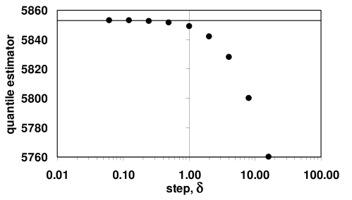
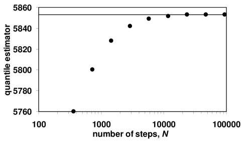
Figure 1: Panjer recursion estimate, $\widehat{q}_{0.999}$, of the 0.999 quantile for the $Poisson(100)-\mathcal{LN}(0,2)$ compound distribution vs the step size $\delta$ (top figure) and vs the number of steps $N=\widehat{q}_{0.999}/\delta$ (bottom figure).

Then the compound discrete density $h_{n}$ is calculated using Panjer recursion and compound distribution is calculated as $H_{n}=\sum_{i=0}^{n}h_{i}$. As an example, Table 2 gives results of calculation of the $Poisson(100)-\mathcal{LN}(0,2)$ compound distribution up to the 0.999 quantile in the case of step $\delta=\text{USD 1}$. Of course the accuracy of the result depends on the step size as shown by the results for the 0.999 quantile vs $\delta$, see Table 3 and Figure 1. It is, however, important to note that the error of the result is due to discretisation only and there is no truncation error (i.e. the severity is not truncated by some large value).

Discretisation can also be done via the forward and backward differences:

$$f_{n}^{U}=F(n\delta+\delta)-F(n\delta);\quad f_{n}^{L}=F(n\delta)-F(n\delta-\delta).$$ (41)

These allow for calculation of the upper and lower bounds for the compound distribution:

$$H_{n}^{U}=\sum_{i=0}^{n}h_{i}^{U};\quad H_{n}^{L}=\sum_{i=0}^{n}h_{i}^{L}.$$ (42)

For example, see Table 4 presenting results for $Poisson(100)-\mathcal{LN}(0,2)$ compound distribution calculated using central, forward and backward differences with step $\delta=\text{USD}1$. The use of the forward difference $f_{n}^{U}$ gives the upper bound for the compound distribution and the use of $f_{n}^{L}$ gives the lower bound. Thus the lower and upper bounds for a quantile are obtained with $f_{n}^{U}$ and $f_{n}^{L}$ respectively. In the case of Table 4 example, the quantile bound interval is [USD 5811, USD 5914] with the estimate from the central difference USD 5849.

5.2 Computational Issues

Underflow in computations of (5.2) will occur for large frequencies during the initialization of the recursion. This can easily be seen for the case of $Poisson(\lambda)$ and $f_{0}=0$ when $h_{0}=\exp(-\lambda)$, that is, the underflow will occur for $\lambda\gtrsim 700$ on a 32bit computer with double precision calculations. Re-scaling $h_{0}$ by large factor $\gamma$ to calculate the recursion (and de-scaling the result) does not really help because overflow will occur for $\gamma h(n)$. The following identity helps to overcome this problem in the case of Poisson frequency:

$$H^{(m)\ast}(z;\lambda/m)=H(z;\lambda).$$ (43)

That is, calculate the compound distribution $H(z;\lambda/m)$ for some large $m$ to avoid underflow. Then preform $m$ convolutions for the obtained distribution directly or via FFT; see Panjer and Willmot (1986). Similar identity is available for negative binomial, $NegBin(r,p)$:

$$H^{(m)\ast}(z;r/m)=H(z;r).$$ (44)

In the case of binomial, $Bin(M,p)$:

$$H^{(m)\ast}(z;m_{1})\ast H(z;m_{2})=H(z;M),$$ (45)

where $m_{1}=\lfloor M/m\rfloor$ and $m_{2}=M-m_{1}m$.

For efficiency, one can choose $m=2^{k}$ so that instead of $m$ convolutions of $H(\cdot)$ only $k$ convolutions are required $H^{(2)\ast},H^{(4)\ast},\ldots,H^{(2^{k})\ast}$, where each term is the convolution of the previous one with itself.

5.3 Panjer Extensions

The Panjer recursion formula (5.2) can be extended to a class of frequency distributions $(a,b,1)$.

Definition 5.5 (Panjer class $(a,b,1)$).

The distribution is said to be in $(a,b,1)$ Panjer class if it satisfies

$$p_{n}=\left(a+\frac{b}{n}\right)p_{n-1},\quad\mbox{for}\quad n\geq 2\quad\mbox{and}\quad a,b\in\mathbb{R}.$$ (46)

Theorem 5.6 (Extended Panjer recursion).

For the frequency distributions in a class $(a,b,1)$:

$$h_{n} = \frac{(p_{1}-(a+b)p_{0})f_{n}+\sum_{j=1}^{n}\left(a+bj/n\right)f_{j}h_{n-j}}{1-af_{0}},\quad n\geq 1,$$

$$h_{0} = \sum\limits_{k=0}^{\infty}{(f_{0})^{k}p_{k}}.$$ (47)

The distributions of $(a,b,0)$ class are special cases of $(a,b,1)$ class. There are two types of frequency distributions in $(a,b,1)$ class:

• zero-truncated distributions, where $p_{0}=0$: i.e. zero truncated Poisson, zero truncated binomial and zero-truncated negative binomial.

• zero-modified distributions, where $p_{0}>0$: the distributions of $(a,b,0)$ with modified probability of zero. It can be viewed as a mixture of $(a,b,0)$ distribution and degenerate distribution concentrated at zero.

Finally, we would like to mention a generalization of Panjer recursion for the $(a,b,l)$ class

$$p_{n}=\left(a+\frac{b}{n}\right)p_{n-1},\quad\mbox{for}\quad n\geq l+1.$$ (48)

For initial values $p_{0}=\cdots=p_{l-1}=0$, and in the case of $f_{0}=0$, it leads to the recursion

$$h_{n}=p_{l}f^{(l)\ast}_{n}+\sum_{j=1}^{n}\left(a+bj/n\right)f_{j}h_{n-j},\quad n\geq l.\\$$

The distribution in this class is, for example, $l-1$ truncated Poisson. For an overview of high order Panjer recursions, see Hess et al (2002). Other types of recursions

$$p_{n}=\sum_{j=1}^{k}(a_{j}+b_{j}/n)p_{n-1},\quad n\geq 1,$$ (49)

are discussed in Sundt (1992). Application of the standard Panjer recursion in the case of the generalised frequency distributions such as the extended negative binomial, can lead to numerical instabilities. Generalization of the Panjer recursion that leads to numerically stable algorithms for these cases is presented in Gerhold et al (2009). Discussion on multivariate version of Panjer recursion can be found in Sundt (1999) and bivariate cases are discussed in Vernic (1999) and Hesselager (1996).

5.4 Panjer Recursion for Continuous Severity

The Panjer recursion is developed for the case of discrete severities. The analog of Panjer recursion for the case of continuous severities is given by the following integral equation.

Theorem 5.7 (Panjer recursion for continuous severities).

For frequency distributions in $(a,b,1)$ class and continuous severity distributions on positive real line:

$$h(z)=p_{1}f(z)+\int_{0}^{x}(a+by/z)f(y)h(z-y)dy.$$ (50)

The proof is presented in Panjer and Willmot (1992, Theorem 6.14.1 and 6.16.1). Note that the above integral equation holds for $(a,b,0)$ class because it is a special case of $(a,b,1)$. The integral equation (50) is a Volterra integral equation of the second type. There are different methods to solve it described in Panjer and Willmot (1992). A method of solving this equation using hybrid MCMC (minimum variance importance sampling via reversible jump MCMC) is presented in Peters et al (2007) .

6 Fast Fourier Transform

The FFT is another efficient method to calculate compound distributions via the inversion of the characteristic function. The method has been known for many decades and originates from the signal processing field. The existence of the algorithm became generally known in the mid-1960s, but it was independently discovered by many researchers much earlier. One of the early books on FFT is Brigham (1974). A detailed explanation of the method in application to aggregate loss distribution can be found in Robertson (1992). In our experience, operational risk practitioners in banking regard the method as difficult and rarely use it in practice. In fact, it is a very simple algorithm to implement, although to make it really efficient, especially for heavy-tailed distribution, some improvements are required. Below we describe the essential steps and theory required for successful implementation of the FFT for operational risk.

As with Panjer recursion case, FFT works with discrete severity and based on the discrete Fourier transformation defined as follows.

Definition 6.1 (Discrete Fourier transformation).

For a sequence $f_{0},f_{1},\ldots,f_{M-1}$, the discrete Fourier transformation (DFT) is defined as

$$\phi_{k}=\sum_{m=0}^{M-1}f_{m}\exp\left(\frac{2\pi i}{M}mk\right),\quad k=0,1,\ldots,M-1$$ (51)

and the original sequence $f_{k}$ can be recovered from $\phi_{k}$ by the inverse transformation

$$f_{k}=\frac{1}{M}\sum_{m=0}^{M-1}\phi_{m}\exp\left(-\frac{2\pi i}{M}mk\right),\quad k=0,1,\ldots,M-1.$$ (52)

Here, $M$ is some truncation point. It is easy to see that to calculate $M$ points of $\phi_{m}$, the number of operations is of the order of $M^{2}$, i.e. $O(M^{2})$. If $M$ is a power of 2, then DFT can be efficiently calculated via FFT algorithms with the number of computations $O(M\log_{2}M)$. This is due to the property that DFT of length $M$ can be represented as the sum of DFT over even points $\phi_{k}^{e}$ and DFT over odd points $\phi_{k}^{e}$:

$$\phi_{k} = \phi_{k}^{e}+\exp\left(\frac{2\pi i}{M}k\right)\phi_{k}^{o};$$

$$\phi_{k}^{e} = \sum_{m=0}^{M/2-1}f_{2m}\exp\left(\frac{2\pi i}{M}mk\right);$$

$$\phi_{k}^{o} = \sum_{m=0}^{M/2-1}f_{2m+1}\exp\left(\frac{2\pi i}{M}mk\right).$$

Subsequently, each of these two DFTs can be calculated as a sum of two DFTs of length $M/4$. For example, $\phi_{k}^{e}$ is calculated as a sum of $\phi_{k}^{ee}$ and $\phi_{k}^{eo}$. This procedure is continued until the transforms of the length 1. The latter is simply identity operation. Thus every obtained pattern of odd and even DFTs will be $f_{m}$ for some $m$:

$$\phi_{k}^{eo\cdots ooe}=f_{m}.$$

The bit reversal procedure can be used to find $m$ that corresponds to a specific pattern. That is, set $e=0$ and $o=1$, then the reverse pattern of $e$’s and $o$’s is the value of $m$ in binary. Thus the logical steps of FFT are as follows.

Algorithm 6.2 (Simple FFT).

1. Sort the data in a bit-reversed order. The obtained points are simply one-point transforms.

2. Combine the neighbor points into non-overlapping pairs to get two-point transforms. Then combine two-point transforms into 4-point transforms and continue subsequently until the final $M$ point transform is obtained. Thus there are $\log_{2}M$ iterations and each iteration involves of the order of $M$ operations.

The implementation of a basic FFT algorithm is very simple; corresponding C or Fortran codes can be found in Press et al (2002, Chapter 12).

6.1 Compound Distribution via FFT

Calculation of the compound distribution via FFT can be done using the following logical steps.

Algorithm 6.3 (Compound Distribution via FFT).

1. Discretise severity to obtain

   $$f_{0},f_{1},\ldots,f_{M-1},$$

   where $M=2^{r}$ with integer $r$ and $M$ is the truncation point in the aggregate distribution;

2. Using FFT, calculate the characteristic function of the severity

   $$\varphi_{0},\ldots,\varphi_{M-1};$$

3. Calculate the characteristic function of the compound distribution using (7), i.e.

   $$\chi_{m}=\psi(\varphi_{m}),\quad m=0,1,\ldots,M-1.$$

4. Perform inverse FFT (which is the same as FFT except the change of sign under the exponent and factor $1/M$) applied to $\chi_{0},\ldots,\chi_{M-1}$ to obtain the compound distribution $h_{0},h_{1},\ldots,h_{M-1}.$

Remarks 6.4.

To calculate the compound distribution in the case of the severity distribution $F(x)$ with a finite support (i.e. $0<a\leq x\leq b<\infty$) one can set $F(x)=0$ for $x$ outside the support range when calculating discretised severity $f_{0},\ldots,f_{M-1}$ using (5.1). For example, this is the case for distribution of losses exceeding some threshold. Note that we need to set $F(x)=0$ in the range $x\in[0,a)$ due to the finite probability of zero compound loss.

6.2 Aliasing Error and Tilting

If there is no truncation error in the severity discretisation, i.e. $\sum_{m=0}^{M-1}f_{m}=1$, then FFT procedure calculates the compound distribution on $m=0,1,\ldots,M$. That is, the mass of compound distribution beyond $M$ is “wrapped” and appears in the range $m=0,\ldots,M-1$ (the so-called aliasing error). This error is larger for heavy-tailed severities. To decrease the error for compound distribution on $0,1,\ldots,n$, one has to take $M$ much larger than $n$. If the severity distribution is bounded and $M$ is larger than the bound, then one can put zero values for points above the bound (the so-called padding by zeros). Another way to reduce the error is to apply some transformation to increase the tail decay (the so-called tilting). The exponential tilting technique for reducing aliasing error under the context of calculating compound distribution was first investigated by Grubel and Hermesmeier (1999). Many authors suggest the following tilting transformation:

$$\widetilde{f}_{j}=\exp(-j\theta)f_{j},\quad j=0,1,\ldots,M-1,$$ (53)

where $\theta>0$. This transformation commutes with convolution in a sense that convolution of two functions $f(x)$ and $g(x)$ equals the convolution of the transformed functions $\widetilde{f}(x)=f(x)\exp(-\theta x)$ and $\widetilde{g}(x)=g(x)\exp(-\theta x)$ multiplied by $\exp(\theta x)$, i.e.

$$(f\ast g)(x)=e^{\theta x}(\widetilde{f}\ast\widetilde{g})(x).$$ (54)

This can easily be shown using the definition of convolution. Then calculation of the compound distribution is performed using the transformed severity distribution as follows.

Algorithm 6.5 (Compound distribution via FFT with tilting).

1. Define $f_{0},f_{1},\ldots,f_{M-1}$ for some large $M$;

2. Perform tilting, i.e. calculate the transformed function $\widetilde{f}_{j}=\exp(-j\theta)f_{j}$, $j=0,1,\ldots,M-1$;

3. Apply FFT to a set $\widetilde{f}_{0},\ldots,\widetilde{f}_{M-1}$ to obtain $\widetilde{\phi}_{0},\ldots,\widetilde{\phi}_{M-1}$;

4. Calculate $\widetilde{\chi}_{m}=\psi(\widetilde{\phi}_{m}),m=0,1,\ldots,M-1$;

5. Apply the inverse FFT to the set $\widetilde{\chi}_{0},\ldots,\widetilde{\chi}_{M-1}$, to obtain $\widetilde{h}_{0},\ldots,\widetilde{h}_{M-1}$;

6. Untilt by calculating final compound distribution as $h_{j}=\widetilde{h}_{j}\exp(\theta j)$.

This tilting procedure is very effective in reducing the aliasing error. The parameter $\theta$ should be as large as possible but not producing under- or overflow that will occur for very large $\theta$. It was reported in Embrechts and Frei (2009) that the choice $M\theta\approx 20$ works well for standard double precision (8 bytes) calculations. Evaluation of the probability generating function $\psi(\cdot)$ of the frequency distribution may lead to the problem of underflow in the case of large frequencies that can be resolved using methods described in Section 5.2.

Example 6.6.

To demonstrate the effectiveness of the tilting, consider the following calculations:

• FFT with the central difference discretisation, where the tail probability compressed into the last point $f_{M-1}=1-F(\delta(M-1)-\delta/2)$. Denote the corresponding quantile estimator as $Q^{(1)}_{0.999}$;

• FFT with the central difference discretisation with the tail probability ignored, i.e. $f_{M-1}=F(\delta(M-1)+\delta/2)-F(\delta(M-1)-\delta/2)$. Denote the corresponding quantile estimator as $Q^{(2)}_{0.999}$;

• FFT with the central difference discretisation utilising tilting $Q^{(tilt)}_{0.999}$. The tilting parameter $\theta$ is chosen to be $\theta=20/M$.

The calculation results presented in Table 5 demonstrate the efficiency of the tilting. If FFT is performed without tilting then the truncation level for the severity should exceed the quantile significantly. In this particular case it should exceed by approximately factor of 10 to get the exact result for this discretisation step. The latter is obtained by Panjer recursion that does not require the discretisation beyond the calculated quantile. Thus the FFT and Panjer recursion are approximately the same in terms of computing time required for quantile estimate in this case. However, once the tilting is utilised, the cut off level does not need to exceed the quantile significantly to obtain the exact result – making FFT superior to Panjer recursion. In this example, the computing time for FFT with tilting is 0.17sec in comparison with 5.76sec of Panjer recursion, see Table 3. Also, in this case, the treatment of the severity tail by ignoring it or absorbing into the last point $f_{M-1}$ does not make any difference when tilting is applied.

7 Direct Numerical Integration

In the case of nonnegative severities, the distribution of the compound loss is given by (15), i.e.

$$H(z)=\frac{2}{\pi}\int\limits_{0}^{\infty}{\mathrm{Re}[\chi(t)]\frac{\sin(tz)}{t}dt},\quad z\geq 0,$$ (55)

where $\chi(t)$ is a compound distribution characteristic function calculated via the severity characteristic function $\varphi(t)$ using (7). For example, the explicit expression of $\mathrm{Re}[\chi(t)]$ for $Poisson(\lambda)$ is

$$\mathrm{Re}[\chi(t)]=e^{-\lambda}\exp(\lambda\mathrm{Re}[\varphi(t)])\times\cos(\lambda\mathrm{Im}[\varphi(t)]).$$ (56)

Hereafter, direct calculation of the distribution function for annual loss $Z$ using (55) is referred to as direct numerical integration (DNI).

Much work has been done in the last few decades in the general area of inverting characteristic functions numerically. Just to mention a few, see the works by Bohman (1975); Seal (1977); Abate and Whitt (1992), (1995); Heckman and Meyers (1983); Shephard (1991); Waller et al (1995); and Den Iseger (2006). These papers address various issues such as singularity at the origin; treatment of long tails in the infinite integration; and choices of quadrature rules covering different objectives with different distributions. Craddock et al (2000) gave an extensive survey of numerical techniques for inverting characteristic functions.

Each of the many existing techniques has particular strengths and weaknesses, and no method works equally well for all classes of problems. In an operational risk context, for instance, there is a special need in computing the 0.999 quantile of the aggregate loss distribution. The accuracy demanded is high and at the same time the numerical inversion could be very time consuming due to rapid oscillations and slow decay in the characteristic function. This is the case, for example, for heavy-tailed severities. Also, the characteristic function of compound distributions should be calculated numerically through semi-infinite integrations. A tailor-made numerical algorithm to integrate (55) was presented in Luo et al (2007) and Luo and Shevchenko (2009) with a specific requirement on accuracy and efficiency in calculating high quantiles such as 0.999 quantile. The method works well for both a wide range of frequencies from very low to very high ($>10^{5}$) and heavy-tailed severities.

7.1 Forward and Inverse Integrations

The task of the characteristic function inversion is analytically straightforward, but numerically difficult in terms of achieving high accuracy and computational efficiency simultaneously.

Accurate calculation of the high quantile as an inverse of the distribution function requires high precision in evaluation of the distribution function. To demonstrate, consider the lognormal distribution $\mathcal{LN}(0,2)$. In this case, the “exact” 0.999 quantile $q_{0.999}=483.2164\ldots$ . However, at $\alpha=0.99902$, the quantile becomes $q_{\alpha}=489.045\ldots\;$. That is, a mere $0.002\%$ change in the distribution function value causes more than $1\%$ change in the quantile value. In the case of a compound distribution, the requirement for accuracy in the distribution function could be even higher, because $1/f(x)$ could be larger at $x=q_{0.999}$. Note that, the error propagation from the distribution function level to the quantile value is implied by the relation between the density $f(x)$ and its distribution function $F(x)$: $dF/dx=f(x)$.

The computation of compound distribution through the characteristic function involves two steps: computing the characteristic function (Fourier transform of the density function, referred to as the forward integration) and inverting it (referred to as the inverse integration).

7.1.1 Forward Integration

This step requires integration (5), that is, calculation of the real and imaginary parts of the characteristic function for a severity distribution:

$$\mathrm{Re}[\varphi(t)]=\int\limits_{0}^{\infty}{f(x)\cos(\,tx)dx},\quad\mathrm{Im}[\varphi(t)]=\int\limits_{0}^{\infty}{f(x)\sin(tx)dx}.$$ (57)

Then, the characteristic function of the compound loss is calculated using (7). These tasks are relatively simple because the severity density typically has closed-form expression, and is well-behaved having a single mode.

This step can be done more or less routinely and many existing algorithms can be employed. The oscillatory nature of the integrand only comes from the sin( ) or cos( ) functions. This well-behaved weighted oscillatory integrand can be effectively dealt with by the modified Clenshaw-Curtis integration method; see Clenshaw and Curtis (1960) and Piessens et al (1983). In this method the oscillatory part of the integrand is transferred to a weight function, the non-oscillatory part is replaced by its expansion in terms of a finite number of Chebyshev polynomials and the modified Chebyshev moments are calculated. If the oscillation is slow when the argument $t$ of the characteristic function is small, the standard Guass-Legendre and Kronrod quadrature formulae are more effective; see Kronrod (1965), Golub and Welsh (1969), Szegö (1975), and Section 7.2. In general, double precision accuracy can be routinely achieved for the forward integrations using standard adaptive integration functions commonly available in many software packages.

7.1.2 Inverse Integration

This step requires integration (55), which is much more challenging task. Changing variable $x=t\times z$, (55) can be rewritten as

$$H(z)=\int_{0}^{\infty}G(x,z)\sin(x)dx,\quad G(x,z)=\frac{2}{\pi}\frac{\mathrm{Re}[\chi(x/z)]}{x},$$ (58)

where $\chi(t)$ depends on $\mathrm{Re}[\varphi(t)]$ and $\mathrm{Im}[\varphi(t)]$ calculated from the forward semi-infinite integrations (57) for any required argument $t$. The total number of forward integrations required by the inversion is usually quite large. This is because in this case the characteristic function could be highly oscillatory due to high frequency and it may decay very slowly due to heavy tails. There are two oscillatory components in the integrand represented by $\sin(x)$ and another part in $\mathrm{Re}[\chi(x/z)]$. It is convenient to treat $\sin(x)$ as the principal oscillatory factor and the other part as secondary. Typically, given $z$, $\mathrm{Re}[\chi(x/z)]$ decays fast initially and then approaches zero slowly as $x$ approaches infinity.

To calculate (58), one could apply the same standard general purpose adaptive integration routines as for the forward integration. However, this is typically not efficient because it does not address irregular oscillation specifically and can lead to an excessive number of integrand evaluations. A simple approach that can be taken is to divide the integration range of (58) into intervals of equal length $\pi$ (referred to as $\pi$-cycle) and truncate at $2K\pi$:

$$H(z)\approx\sum\limits_{k=0}^{2K-1}{H_{k}},\quad H_{k}=\int\limits_{k\pi}^{(k+1)\pi}{G(x)\sin(x)dx}.$$ (59)

Within each $\pi$-cycle, the secondary oscillation could be dominating for some early cycles, thus the $\pi$-cycle could in fact contain multiple cycles due to the “secondary” oscillation. Thus a further sub-division is warranted. Sub-dividing interval $\left(k\pi,\;(k+1)\pi\right)$ into $n_{k}$ segments of equal length of $\Delta_{k}=\pi/n_{k}$, (59) can be written as

$$H_{k}=\sum\limits_{j=1}^{n_{k}}{H_{k}^{(j)},\quad H_{k}^{(j)}=\int\limits_{a_{k,j}}^{b_{k,j}}{G(x)\sin(x)dx}},$$ (60)

where

$$a_{k,j}=k\pi+(j-1)\Delta_{k},\quad b_{k,j}=a_{k,j}+\Delta_{k}.$$

The above calculation will be most effective if the sub-division is made adaptive for each $\pi$-cycle according to the changing behaviour of $G(x)$. Assuming that for the first $\pi$-cycle ($k=0)$ we have initial partition $n_{0}$, Luo and Shevchenko (2009) recommends making $n_{k}$ adaptive for the subsequent cycles by the following two simple rules:

• Let $n_{k}$ be proportional to the number of $\pi$-cycles of the secondary oscillation – the number of oscillations in $G(x)$ within each principal $\pi$-cycle;

• Let $n_{k}$ be proportional to the magnitude of the maximum gradient of $G(x)$ within each principal $\pi$-cycle.

Application of these rules requires correct counting of secondary cycles and good approximation of the local gradient in $G(x)$. Both can be achieved with a significant number of points at which $G(x)$ is computed within each cycle using, for example, the $m$-point Gaussian quadrature described in the next section.

7.2 Gaussian Quadrature for Subdivisions

With a proper sub-division, even a simple trapezoidal rule can be applied to get a good approximation for integration over the sub-division $H_{k}^{(j)}$ in (60). However, higher order numerical quadrature can achieve higher accuracy for the same computing effort or it requires less computing effort for the same accuracy. The $m$-point Gaussian quadrature makes the computed integral exact for all polynomials of degree 2$m-$1 or less. In particular:

$$\int_{a}^{b}g(x)dx\approx\frac{\Delta}{2}\sum_{i=1}^{m}w_{i}g\left((a+b+\zeta_{i}\Delta)/2\right),$$ (61)

where $0<w_{i}<1$ and $-1<\zeta_{i}<1$ are the $i^{th}$ weight and the $i^{th}$ abscissa of the Gaussian quadrature respectively, $\Delta=b-a$ and $m$ is the order of the Gaussian quadrature.

Typically, even a simple 7-point Gaussian quadrature ($m=7)$, which calculates all polynomials of degree 13 or less exactly, can successfully be used to calculate $H_{k}^{(j)}$ in (59, 60). For completeness, Table 6 presents 7-point Gaussian quadrature weights and abscissas; other quadratures can be found in Piessens et al (1983).

The efficiency of the Gaussian quadrature is much superior to the trapezoidal rule. For instance, integrating the function $\sin(3x)$ over the interval $(0,\pi)$, the 7-point Gaussian quadrature has a relative error less than $10^{-5}$, while the trapezoidal rule requires about 900 function evaluations (grid spacing $\delta x=\pi/900)$ to achieve a similar accuracy. The reduction of the number of integrand function evaluations is important for a fast integration of (59), because the integrand itself is a time consuming semi-infinite numerical integration.

The error of the $m$-point Gaussian quadrature rule can be accurately estimated if the 2$m$ order derivative of the integrand can be computed (Kahaner et al (1989); Stoer and Bulirsch (2002)). In general, it is difficult to estimate the $2m$ order derivative and the actual error may be much less than a bound established by the derivative. As it has already been mentioned, a common practice is to use two numerical evaluations with the grid sizes different by the factor of two and estimate the error as the difference between the two results. Equivalently, different orders of quadrature can be used to estimate error. Often, Guass-Kronrod quadrature is used for this purpose. Adaptive integration functions in many numerical software packages use this estimate to achieve an overall error bound below the user-specified tolerance.

7.3 Tail Integration

The truncation error of using (59) is

$$H_{T}=\int\limits_{2K\pi}^{\infty}{G(x)\sin(x)dx}.$$ (62)

For higher accuracy, instead of increasing truncation length at the cost of computing time, one can try to calculate the tail integration $H_{T}$ approximately or use tilting transform (53). Integration of (62) by parts gives

$$\int\limits_{2K\pi}^{\infty}G(x)\sin(x)dx = G(2K\pi)+\sum_{j=1}^{k-1}(-1)^{j}G^{(2j)}(2K\pi)$$ (63)

$$+(-1)^{k}\int_{2K\pi}^{\infty}G^{(2k)}(x)\sin(x)dx,$$

where $k\geq 1$, $G^{(2j)}(2K\pi)$ is the $2j$-th order derivative of $G(x)$ at the truncation point. Under some conditions, as $K\to\infty$,

$$\int\limits_{2K\pi}^{\infty}G(x)\sin(x)dx\to G(2K\pi)+\sum_{j=1}^{\infty}(-1)^{j}G^{(2j)}(2K\pi).$$

For example, if we assume that for some $\gamma<0$, $G^{(m)}(x)=O(x^{\gamma-m})$, $m=0,1,2,\ldots$ as $K\to\infty$, then the series converges to the integral. However, this is not true for some functions, such as $\exp(-x)$; typically in this case the truncation error is not material. It appears that often, the very first term in (63) gives a very good approximation

$$H_{T}=\int\limits_{2K\pi}^{\infty}{G(x)\sin(x)dx}\approx G(2K\pi)$$ (64)

for the tail integration or does not have a material impact on the overall integration; see Luo and Shevchenko (2009, 2010). This elegant result means that we only need to evaluate the integrand at one single point $x=2\pi K$ for the entire tail integration. Thus the total integral approximation (59) can be improved by including tail correction giving

$$H(z)\approx\sum\limits_{k=0}^{2K-1}H_{k}+G(2N\pi).$$ (65)

Remarks 7.1.

The approximation (64) can be improved by including further terms if derivatives are easy to calculate, e.g. $H_{T}\approx G(2K\pi)-G^{(2)}(2K\pi)$. If the oscillating factor is $\cos(x)$ instead of $\sin(x)$, one can still derive a one-point formula similar to (63) by starting the tail integration at $(2K-1/2)\pi$ instead of $2K\pi$.

Of course there are more elaborate methods to treat the truncation error which are superior to a simple approximation (64) in terms of better accuracy and broader applicability, such as some of the extrapolation methods proposed in Wynn (1956), Sidi (1980) and Sidi (1988).

7.4 Error Sources and Numerical Example

Table 7 shows the convergence of DNI results (seven digits), for truncation lengths $2\leq K\leq 80$ in the cases of tail correction included and ignored. One can see a material improvement from the tail correction. Also, as the truncation length increases, both estimators with the tail correction and without converge. In this particular case we calculate compound distribution $Poisson(100)$-$\mathcal{LN}(0,2)$ at the level $z=5853.1$. The latter is the value that corresponds to the 0.999 quantile (within 1st decimal place) of this distribution as has already been calculated by Panjer recursion; see Table 3. Of course, to calculate the quantile at the 0.999 level using DNI, a search algorithm such as bisection should be used that will require evaluation of distribution function many times (of the order of 10) increasing computing time. Comparing this with Tables 3 and 5, one can see that for this case DNI is faster than Panjer recursion while slower than FFT (with tilting) by a factor of 10.

The final result of the inverse integration has three error sources: the discretisation error of the Gauss quadrature; the error from the tail approximation; and the error propagated from the error of the forward integration. These were analysed in Luo and Shevchenko (2009). It was shown that the propagation error is proportional to the forward integration error bound. At the extreme case of $\lambda=10^{6}$, a single precision can still be readily achieved if the forward integration has a double precision. For very large $\lambda$, the propagation error is likely the largest among the three error sources. Though some analytic formulas for error bounds are available, these are not very useful in practise because high order derivatives are involved, which is typical for analytical error bounds. An established and satisfactory practice is to use finer grids to estimate the error of the coarse grids.

8 Comparison of Numerical Methods

For comparison purposes, Tables 8 and 9 present results for the 0.999 quantile of compound distributions $Poisson(\lambda)$-$\mathcal{LN}(0,2)$ and $Poisson(\lambda)$-${GPD}(1,1)$ (with $\lambda=0.1,10,10^{3}$), calculated by the DNI, FFT, Panjer and MC methods. Note that, with the shape parameter $\xi=1$, $GPD(\xi,\beta)$ has infinite mean and all higher moments. For DNI, FFT and Panjer recursion methods, the results, accurate up to 5 significant digits, were obtained as follows:

• For DNI algorithm we start with a relatively coarse grid ($n_{0}=1$) and short truncation length $K=25$, and keep halving the grid size and doubling the truncation length until the difference in the 0.999 quantile is within required accuracy. The DNI algorithm computes distribution function, $H(z)$, for any given level $z$ by (55), one point at a time. Thus with DNI we have to resort to an iterative procedure to inverse (55). This requires evaluating (55) many times depending on the search algorithm employed and the initial guess. Here, a standard bisection algorithm is employed. Other methods (MC, Panjer recursion and FFT) have the advantage that they obtain the whole distribution in a single run.

• For Panjer recursion, starting with a large step (e.g. $\delta=8$) the step $\delta$ is successively reduced until the change in the result is smaller than the required accuracy.

• For FFT with tilting, the same step $\delta$ is used as the one in the Panjer recursion. If we would not know the Panjer recursion results, then we would successively reduce the step $\delta$ (starting with some large step) until the change in the result is smaller than the required accuracy. The truncation length $M=2^{r}$ has to be large enough so that $\delta M>\widehat{Q}_{q}$ is satisfied. We use the smallest possible integer $r$ that allows to identify the quantile, typically such that $\delta M\approx 2\widehat{Q}_{q}$. Here, $\widehat{Q}_{q}$ is the quantile to be computed, which is not known a priori and some extra iteration is typically required. Also, the tilting parameter is set to $\theta=20/M$.

• For the MC estimates, the number of simulations, $N_{MC}$ (denoted by $K$ in Section 4), ranges from $10^{6}$ to $10^{8}$, so that calculations are accomplished within $\approx 10$ min. The error of the MC estimate is approximately proportional to $1/\sqrt{N_{MC}}$ and the calculation time is approximately proportional to $N_{MC}$. Thus the obtained results allow to judge how many simulations (time) is required to achieve a specific accuracy.

The agreement between FFT, Panjer recursion and DNI estimates is perfect. Also, the difference between these results and corresponding MC estimates is always within the two MC standard errors. However, the CPU time is very different across the methods:

• The quoted CPU time for the MC results is of the order 10 min. However, it is clear from the standard error results (recalling that the error is proportional to $1/\sqrt{N_{MC}}$) that the CPU time, required to get the results accurate up to five significant digits, would be of the order of several days. Thus MC is the slowest method.

• Typically, the CPU time for both Panjer recursion and FFT increase as $\lambda$ increases, while CPU time for DNI does not change significantly.

• FFT is the fastest method, though at very high frequency $\lambda=10^{3}$, DNI performance is of a similar order. As reported in Luo and Shevchenko (2009), DNI becomes faster than FFT for higher frequencies $\lambda>10^{3}$.

• Panjer recursion is always slower than FFT. It is faster than DNI for small frequencies and much slower for high frequencies.

Finally note that, the FFT, Panjer recursion and DNI results were obtained by successive reduction of grid size (starting with a coarse grid) until the required accuracy is achieved. The quoted CPU time is for the last iteration in this procedure. Thus the results for CPU time should be treated as indicative only. For comparison of FFT and Panjer, also see Embrechts and Frei (2009), and Bühlmann (1984).

9 Closed-Form Approximation

There are several well-known approximations for the compound loss distribution. These can be used with different success depending on the quantity to be calculated and distribution types. Even if the accuracy is not good, these approximations are certainly useful from the methodological point of view in helping to understand the model properties. Also, the quantile estimate derived from these approximations can successfully be used to set a cut-off level for FFT algorithms that will subsequently determine the quantile more precisely.

9.1 Normal and Translated Gamma Approximations

Many parametric distributions can be used as an approximation for a compound loss distribution by moment matching. This is because the moments of the compound loss can be calculated in closed-form. In particular, the first four moments are given in Proposition 2.2. Of course these can only be used if the required moments exist which is not the case for some heavy-tailed risks with infinite moments. Below we mention normal and translated gamma approximations, discussed e.g. in McNeil et al (2005, Section 10.2.3).

9.1.1 Normal Approximation

As the severities $X_{1},X_{2},\ldots\;$ are independent and identically distributed, at very high frequencies the central limit theory is expected to provide a good approximation to the distribution of the annual loss $Z$ (if the second moment of severities is finite). Then the compound distribution is approximated by the normal distribution with the mean and variance given in Proposition 2.2, that is,

$$H(z)\approx\mathcal{N}(\mathrm{E}[Z],\sqrt{\mathrm{Var}[Z]}).$$ (66)

This is an asymptotic result and a priori we do not know how well it will perform for a specific distribution types and distribution parameter values. Also, it cannot be used for the cases where variance or mean are infinite.

Example 9.1.

If $N$ is distributed from $Poisson(\lambda)$ and $X_{1},\ldots,X_{N}$ are independent random variables from $\mathcal{LN}(\mu,\sigma)$, then

$$\mathrm{E}[Z]=\lambda\exp(\mu+0.5\sigma^{2}),\quad\mathrm{Var}[Z]=\lambda\exp(2\mu+2\sigma^{2}).$$ (67)

9.1.2 Translated Gamma Approximation

From (2.3), the skewness of the compound distribution, in the case of Poisson distributed frequencies, is

$$\frac{\mathrm{E}[(Z-\mathrm{E}[Z])^{3}]}{\left(\mathrm{Var}[Z]\right)^{3/2}}=\frac{\lambda\mathrm{E}[X^{3}]}{\left(\lambda\mathrm{E}[X^{2}]\right)^{3/2}}>0,$$ (68)

that approaches zero as $\lambda$ increases but finite positive for finite $\lambda>0$. To improve the normal approximation (66), the compound loss can be approximated by the shifted gamma distribution which has a positive skewness, that is, $Z$ is approximated as $Y+a$ where $a$ is a shift and $Y$ is a random variable from $Gamma(\alpha,\beta)$. The three parameters are estimated by matching the mean, variance and skewness of the approximate distribution and the correct one:

$$a+\alpha\beta=\mathrm{E}[Z];\quad\alpha\beta^{2}=\mathrm{Var}[Z];\quad\frac{2}{\sqrt{\alpha}}=\mathrm{E}[(Z-\mathrm{E}[Z])^{3}]/\left(\mathrm{Var}[Z]\right)^{3/2}.$$ (69)

This approximation requires the existence of the first three moments and thus cannot be used if the third moment does not exist.

Example 9.2.

If frequencies are Poisson distributed, $N\sim Poisson(\lambda)$, then

$$a+\alpha\beta=\lambda\mathrm{E}[X];\quad\alpha\beta^{2}=\lambda\mathrm{E}[X^{2}];\quad\frac{2}{\sqrt{\alpha}}=\lambda\mathrm{E}[X^{3}]/\left(\lambda\mathrm{E}[X^{2}]\right)^{3/2}.$$ (70)

9.2 VaR Closed-Form Approximation

If severities $X_{1},\ldots,X_{N}$ are independent and identically distributed from the sub-exponential (heavy tail) distribution $F(x)$, and frequency distribution satisfies

$$\sum_{n=0}^{\infty}(1+\epsilon)^{n}\Pr[N=n]<\infty$$

for some $\epsilon>0$, then the tail of the compound distribution $H(z)$, of the compound loss $Z=X_{1}+\cdots+X_{N}$, is related to the severity tail as

$$1-H(z)\to\mathrm{E}[N](1-F(z)),\quad\mbox{as}\quad z\to\infty;$$ (71)

see Theorem 1.3.9 in Embrechts et al (1997). The validity of this asymptotic result was demonstrated for the cases when $N$ is distributed from Poisson, binomial or negative binomial. It can be used to find the quantile of the annual loss

$$\mathrm{VaR}_{\alpha}[Z]\to F^{-1}\left({1-\frac{1-\alpha}{\mathrm{E}[N]}}\right),\quad\mbox{as}\quad\alpha\to 1.$$ (72)

For application in the operational risk context, see Böcker and Klüppelberg (2005). Under the assumption that the severity has a finite mean, Böcker and Sprittulla (2006) derived a correction reducing the approximation error of (72).

Example 9.3.

Consider a heavy-tailed compound distribution $Poisson(\lambda)$-${GPD}(\xi,\beta)$. In this case, (72) gives

$$\mathrm{VaR}_{\alpha}[Z]\to\frac{\beta}{\xi}\left({\frac{\lambda}{1-\alpha}}\right)^{\xi},\quad\mbox{as}\quad\alpha\to 1.$$ (73)

This implies a simple scaling, $\mathrm{VaR}_{\alpha}[Z]\propto\lambda^{\xi}$, with respect to the event intensity $\lambda$ for large $\alpha$.

Example 9.4.

To demonstrate the accuracy the above approximations, consider compound distribution $Poisson(\lambda=100)$-$\mathcal{LN}(\mu=0,\sigma=2)$ with relatively heavy tail severity. Calculating moments of the lognormal distribution $\mathrm{E}[X^{m}]$ using (23) and substituting into (2.3) gives

$$\mathrm{E}[Z]\approx 738.9056,\quad\mathrm{Var}[Z]\approx 298095.7987,$$

$$\mathrm{E}[(Z-\mathrm{E}[Z])^{3}]/(\mathrm{Var}[Z])^{3/2}\approx 40.3428.$$

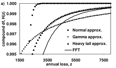
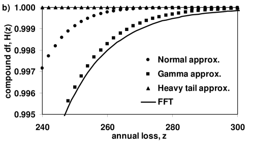
Figure 2: Different approximations for the tail of the $Poisson(100)-\mathcal{LN}(0,\sigma)$ distribution for a) $\sigma=2$; and b) less heavier tail $\sigma=1$.

Approximating the compound distribution by the normal distribution with these mean and variance gives normal approximation. Approximating the compound distribution by the translated gamma distribution (69) with these mean, variance and skewness gives: $\alpha\approx 0.002457$, $\beta\approx 11013.2329$, $a\approx 711.8385$. Figure 2a shows the normal and translated gamma approximations for the tail of the compound distribution. These are compared with the asymptotic result for heavy tail distributions (71) and “exact” values obtained by FFT. It is easy to see that the heavy tail asymptotic approximation (71) converges to the “exact” result for large quantile level $\alpha\to 1$, while the normal and gamma approximations perform badly. The results for the case of not so heavy tail, when the severity distribution is $\mathcal{LN}(0,1)$, are shown in Figure 2b. Here, the gamma approximation outperforms normal approximation and heavy tail approximation is very bad. The accuracy of the heavy tail approximation (71) improves for more heavy-tailed distributions, such as GPD with infinite variance or even infinite mean.

10 Conclusions

In this paper we reviewed methods that can be used to calculate the distribution of the compound loss. Overall, FFT with tilting is typically the fastest method though it involves tuning of the cut-off level, tilting parameter and discretisation step. The easiest to implement is Panjer recursion that involves discretisation error only. DNI method is certainly competitive with FFT and Panjer for large frequencies, though its implementation can be quite involved. Monte Carlo method is slow but simple in implementation and it can easily handle multiple risks with dependence. The latter is problematic for FFT and Panjer recursion methods. In general, each of the reviewed techniques has particular strengths and weaknesses that a modeller should be aware of. The choice of the method is dictated by the specific objectives to be achieved.

Appendix A List of Distributions

Poisson distribution, $Poisson(\lambda)$. A Poisson distribution function is denoted as $Poisson(\lambda)$. The random variable $N$ has a Poisson distribution, denoted $N\sim Poisson(\lambda)$, if its probability mass function is

$$p_{k}=\Pr[N=k]=\frac{\lambda^{k}}{k!}e^{-\lambda},\;\lambda>0,\;k\in\{0,1,2,\ldots\}.$$ (74)

Expectation, variance and variational coefficient are

$$\mathrm{E}[N]=\lambda,\;\mathrm{Var}[N]=\lambda,\;\mathrm{Vco}[N]=\frac{1}{\sqrt{\lambda}}.$$ (75)

Binomial distribution, $Bin(n,p)$. A binomial distribution function is denoted as $Bin(n,p)$. The random variable $N$ has a binomial distribution, denoted $N\sim Bin(n,p)$, if its probability mass function is

$$p_{k}=\Pr[N=k]=\left(\begin{array}[]{c}n\\ k\end{array}\right)p^{k}(1-p)^{n-k},\;p\in(0,1),\;n\in{1,2,\ldots}$$ (76)

for all $k\in\{0,1,\ldots,n\}$. Expectation, variance and variational coefficient are

$$\mathrm{E}[N]=np,\;\mathrm{Var}[N]=np(1-p),\;\mathrm{Vco}[N]=\sqrt{\frac{1-p}{np}}.$$ (77)

Negative binomial distribution, $NegBin(r,p)$. A negative binomial distribution function is denoted as $NegBin(r,p)$. The random variable $N$ has a negative binomial distribution, denoted $N\sim NegBin(r,p)$, if its probability mass function is

$$p_{k}=\Pr[N=k]=\frac{\mathrm{\Gamma}(k+r)}{k!\mathrm{\Gamma}(r)}p^{r}(1-p)^{k},\;p\in(0,1),\;r\in(0,\infty)$$ (78)

for all $k\in\{0,1,2,\ldots\}$. Here, $\mathrm{\Gamma}(r)$ is the gamma function. Expectation, variance and variational coefficient are

$$\mathrm{E}[N]=\frac{r(1-p)}{p},\mbox{ }\mathrm{Var}[N]=\frac{r(1-p)}{p^{2}},\;\mathrm{Vco}[N]=\frac{1}{\sqrt{r(1-p)}}.$$ (79)

Normal distribution, ${\mathcal{N}}(\mu,\sigma)$. A normal (Gaussian) distribution function is denoted as ${\mathcal{N}}(\mu,\sigma)$. The random variable $X$ has a normal distribution, denoted $X\sim{\mathcal{N}}(\mu,\sigma)$, if its probability density function is

$$f(x)=\frac{1}{\sqrt{2\pi\sigma^{2}}}\mathrm{exp}\left(-\frac{(x-\mu)^{2}}{2\sigma^{2}}\right),\;\sigma^{2}>0,\;\mu\in\mathbb{R}$$ (80)

for all $x\in\mathbb{R}$. Expectation, variance and variational coefficient are

$$\mathrm{E}[X]=\mu,\;\mathrm{Var}[X]=\sigma^{2},\;\mathrm{Vco}[X]=\sigma/\mu.$$ (81)

Lognormal distribution, ${\mathcal{L}N}(\mu,\sigma)$ A lognormal distribution function is denoted as ${\mathcal{L}N}(\mu,\sigma)$. A random variable $X$ has a lognormal distribution, denoted $X\sim{\mathcal{LN}}(\mu,\sigma)$, if its probability density function is

$$f(x)=\frac{1}{x\sqrt{2\pi\sigma^{2}}}\mathrm{exp}\left(-\frac{(\ln(x)-\mu)^{2}}{2\sigma^{2}}\right),\;\sigma^{2}>0,\;\mu\in\mathbb{R}$$ (82)

for $x>0$. Expectation, variance and variational coefficient are

$$\mathrm{E}[X]=e^{\mu+\frac{1}{2}\sigma^{2}},\;\mathrm{Var}[X]=e^{2\mu+\sigma^{2}}(e^{\sigma^{2}}-1),\;\mathrm{Vco}[X]=\sqrt{e^{\sigma^{2}}-1}.$$ (83)

Gamma distribution, $Gamma(\alpha,\beta)$. A gamma distribution function is denoted as $Gamma(\alpha,\beta)$. The random variable $X$ has a gamma distribution, denoted as $X\sim Gamma(\alpha,\beta)$, if its probability density function is

$$f(x)=\frac{x^{\alpha-1}}{\mathrm{\Gamma}(\alpha)\beta^{\alpha}}\exp(-x/\beta),\;\alpha>0,\;\beta>0$$ (84)

for $x>0$. Expectation, variance and variational coefficient are

$$\mathrm{E}[X]=\alpha\beta,\;\mathrm{Var}[X]=\alpha\beta^{2},\;\mathrm{Vco}[X]=1/\sqrt{\alpha}.$$ (85)

Generalised Pareto distribution, $GPD(\xi,\beta)$. The GPD distribution function is denoted as $GPD(\xi,\beta)$. The random variable $X$ has GPD distribution, denoted as $X\sim GPD(\xi,\beta)$, if its distribution function is

$$H_{\xi,\beta}(x)=\left\{\begin{array}[]{ll}1-(1+\xi x/\beta)^{-1/\xi},&\xi\neq 0,\\ 1-\exp(-x/\beta),&\xi=0,\\ \end{array}\right.$$ (86)

where $x\geq 0$ when $\xi\geq 0$ and $0\leq x\leq-\beta/\xi$ when $\xi<0$. The moments of $X\sim GPD(\xi,\beta)$, $\xi\geq 0$, can be calculated using

$$\mathrm{E}[X^{n}] = \frac{\beta^{n}n!}{\prod_{k=1}^{n}(1-k\xi)},\;\xi<\frac{1}{n}.$$ (87)

Table 1: Panjer recursion starting values $h_{0}$ and $(a,b)$ parameters for Poisson, binomial and negative binomial distributions.

	$a$	$b$	$h_{0}$
$Poisson(\lambda)$	$0$	$\lambda$	$\exp(\lambda(f_{0}-1))$
$NegBin(r,q)$	$1-q$	$(1-q)(r-1)$	$\left(1+(1-f_{0})\frac{1-q}{q}\right)^{-r}$
$Bin(m,q)$	$-\frac{q}{1-q}$	$\frac{q(m+1)}{1-q}$	$(1+q(f_{0}-1))^{m}$

Table 2: Example of Panjer recursion calculating the $Poisson(100)-\mathcal{LN}(0,2)$ compound distributions using central difference discretisation with the step $\delta=1$.

$n$	$f_{n}$	$h_{n}$	$H_{n}$
$0$	$0.364455845$	$2.50419\times 10^{-28}$	$2.50419\times 10^{-28}$
$1$	$0.215872117$	$5.40586\times 10^{-27}$	$5.65628\times 10^{-27}$
$2$	$0.096248034$	$6.07589\times 10^{-26}$	$6.64152\times 10^{-26}$
$\vdots$	$\vdots$	$\vdots$	$\vdots$
$5847$	$2.81060\times 10^{-9}$	$4.44337\times 10^{-7}$	$0.998999329$
$5848$	$2.80907\times 10^{-9}$	$4.44061\times 10^{-7}$	$0.998999773$
$5849$	$2.80755\times 10^{-9}$	$4.43785\times 10^{-7}$	$0.999000217$

Table 3: Convergence of Panjer recursion estimate, $\widehat{q}_{0.999}$, of the 0.999 quantile for the $Poisson(100)-\mathcal{LN}(0,2)$ compound distributions using central difference discretisation vs the step size $\delta$. Here, $N=\widehat{q}_{0.999}/\delta$ is the number of steps required.

$\delta$	$N$	$\widehat{q}_{0.999}$	time(sec)
$16$	$360$	$5760$	$0.19$
$8$	$725$	$5800$	$0.20$
$4$	$1457$	$5828$	$0.28$
$2$	$2921$	$5842$	$0.55$
$1$	$5849$	$5849$	$1.59$
$0.5$	$11703$	$5851.5$	$5.77$
$0.25$	$23411$	$5852.75$	$22.47$
$0.125$	$46824$	$5853$	$89.14$
$0.0625$	$93649$	$5853.0625$	$357.03$

Table 4: Example of Panjer recursion calculating the $Poisson(100)-\mathcal{LN}(0,2)$ compound distributions using central, forward and backward difference discretisation with the step $\delta=1$.

$n$	$H_{n}^{L}$	$H_{n}$	$H_{n}^{U}$
$0$	$3.72008\times 10^{-44}$	$2.50419\times 10^{-28}$	$1.92875\times 10^{-22}$
$1$	$1.89724\times 10^{-42}$	$5.65628\times 10^{-27}$	$2.80718\times 10^{-21}$
$\vdots$	$\vdots$	$\vdots$	$\vdots$
$5811$	$0.998953196$	$0.998983158$	$0.998999719$
$5812$	$0.998953669$	$0.998983612$	$0.999000163$
$\vdots$	$\vdots$	$\vdots$	$\vdots$
$5848$	$0.9989705$	$0.998999773$	$0.999015958$
$5849$	$0.998970962$	$0.999000217$	$0.999016392$
$\vdots$	$\vdots$	$\vdots$	$\vdots$
$5913$	$0.998999942$	$0.999028056$	$0.999043605$
$5914$	$0.999000385$	$0.999028482$	$0.999044022$

Table 5: Example of FFT calculating the 0.999 quantile of the $Poisson(100)-\mathcal{LN}(0,2)$ compound distribution using central difference discretisation with the step $\delta=0.5$. The exact Panjer recursion for this discretisation step gives $Q_{0.999}=5851.5$.

$r$	$L=\delta\times 2^{r}$	$Q^{(1)}_{0.999}$	$Q^{(2)}_{0.999}$	$Q^{(tilt)}_{0.999}$	time (sec)
$14$	$8192$	$5117$	$5665.5$	$5851.5$	$0.17$
$15$	$16384$	$5703.5$	$5834$	$5851.5$	$0.36$
$16$	$32768$	$5828$	$5850$	$5851.5$	$0.75$
$17$	$65536$	$5848.5$	$5851.5$	$5851.5$	$1.61$
$18$	$131072$	$5851.5$	$5851.5$	$5851.5$	$3.64$
$19$	$262144$	$5851.5$	$5851.5$	$5851.5$	$7.61$

Table 6: The weights $w_{i}$ and abscissas $\zeta_{i}$ of the 7-point Gaussian quadrature

$i$	$\zeta_{i}$	$w_{i}$
$1$	-0.949107912342759	0.129484966168870
$2$	-0.741531185599394	0.279705391489277
$3$	-0.405845151377397	0.381830050505119
$4$	0.0	0.417959183673469
$5$	0.405845151377397	0.381830050505119
$6$	0.741531185599394	0.279705391489277
$7$	0.949107912342759	0.129484966168870

Table 7: Convergence in DNI estimates of $H(z=5853.1)$ for $Poisson(100)$-$\mathcal{LN}(0,2)$ in the case of $n_{0}=1$ and different truncation length $K$. $\widehat{H}_{tail}$ is the estimate with the tail correction and $\widehat{H}$ is the estimate without the tail correction.

$K$	$\widehat{H}$	$\widehat{H}_{tail}$	time(sec)
2	0.9938318	0.9999174	0.0625
3	1.0093983	0.9993260	0.094
4	1.0110203	0.9991075	0.125
5	1.0080086	0.9990135	0.141
10	0.9980471	0.9989910	0.297
20	0.9990605	0.9990002	0.578
40	0.9989996	0.9990000	1.109
80	0.9990000	0.9990000	2.156

Table 8: The estimates of the 0.999 quantile, ${Q}_{0.999}$, for $Poisson(\lambda)$-$\mathcal{LN}(0,2)$, calculated using DNI, FFT, Panjer recursion and MC methods. Standard errors of MC estimates are given in brackets next to the estimator.

	$\lambda$	0.1	10	1000
DNI	$Q_{0.999}$	$105.36$	$1,779.1$	$21,149$
	time	15.6s	6s	25s
	$K\backslash n_{0}$	$50\backslash 2$	$25\backslash 1$	$25\backslash 1$
MC	$Q_{0.999}$	$105.45(0.26)$	$1,777(9)$	$21,094(185)$
	time	3min	3.9min	11.7min
	$N_{MC}$	$10^{8}$	$10^{7}$	$10^{6}$
Panjer	$Q_{0.999}$	$105.36$	$1,779.1$	$21,149$
	time	7.6s	8.5s	3.6h
	$h$	$2^{-7}$	$2^{-3}$	$2^{-4}$
FFT	$Q_{0.999}$	$105.36$	$1,779.1$	$21,149$
	time	0.17s	0.19s	7.9s
	$h$	$2^{-7}$	$2^{-3}$	$2^{-4}$
	$M$	$2^{14}$	$2^{14}$	$2^{19}$

Table 9: The estimates of the 0.999 quantile, ${Q}_{0.999}$, for $Poisson(\lambda)$-$GPD(1,1)$, calculated using DNI, FFT, Panjer recursion and MC methods. Standard errors of MC estimates are given in brackets next to the estimator.

	$\lambda$	0.1	10	1000
DNI	$Q_{0.999}$	$99.352$	$10,081$	$1.0128\times 10^{6}$
	time	21s	29s	52s
	$K\backslash n_{0}$	$100\backslash 2$	$100\backslash 2$	$100\backslash 1$
MC	$Q_{0.999}$	$99.9(0.3)$	$10,167(89)$	$1.0089(0.026)\times 10^{6}$
	time	3.1min	3.6min	7.8min
	$N_{MC}$	$10^{8}$	$10^{7}$	$10^{6}$
Panjer	$Q_{0.999}$	$99.352$	$10,081$	$1.0128\times 10^{6}$
	time	6.9s	4.4s	15h
	$h$	$2^{-7}$	$1$	$1$
FFT	$Q_{0.999}$	99.352	$10,081$	$1.0128\times 10^{6}$
	time	0.13s	0.13s	28s
	$h$	$2^{-7}$	$1$	$1$
	$M$	$2^{14}$	$2^{14}$	$2^{21}$

References

- [1] Abate, J. and Whitt, W. (1992) Numerical inversion of laplace transforms of probability distributions. ORSA Journal of Computing 7, 36–43.
- [2] Abate, J. and Whitt, W. (1995) Numerical inversion of probability generating functions. Operations Research Letters 12, 245–251.
- [3] Bladt, M. (2005) A review of phase-type distributions and their use in risk theory. ASTIN Bulletin 35(1), 145–167.
- [4] Böcker, K. and Klüppelberg, C. (2005) Operational VAR: a closed-form approximation. Risk Magazine 12, 90–93.
- [5] Böcker, K. and Sprittulla, J. (2006) Operational VAR: meaningful means. Risk Magazine 12, 96–98.
- [6] Bohman, H. (1975) Numerical inversion of characteristic functions. Scandinavian Actuarial Journal pp. 121–124.
- [7] Brigham, E. O. (1974) The Fast Fourier Transform. Prentice-Hall, Englewood Cliffs, NJ.
- [8] Bühlmann, H. (1984) Numerical evaluation of the compound Poisson distribution: recursion or Fast Fourier Transform? Scandinavian Actuarial Journal pp. 116–126.
- [9] Chernobai, A. S., Rachev, S. T. and Fabozzi, F. J. (2007) Operational Risk: A Guide to Basel II Capital Requirements, Models, and Analysis. John Wiley & Sons, New Jersey.
- [10] Clenshaw, C. W. and Curtis, A. R. (1960) A method for numerical integration on an automatic computer. Num. Math 2, 197–205.
- [11] Craddock, M., Heath, D. and Platen, E. (2000) Numerical inversion of Laplace transforms: a survey of techniques with applications to derivative pricing. Computational Finance 4(1), 57–81.
- [12] Den Iseger, P. W. (2006) Numerical Laplace inversion using Gaussian quadrature. Probability in the Engineering and Informational Sciences 20, 1–44.
- [13] Embrechts, P. and Frei, M. (2009) Panjer recursion versus FFT for compound distributions. Mathematical Methods of Operations Research 69(3), 497–508.
- [14] Embrechts, P., Klüppelberg, C. and Mikosch, T. (1997) Modelling Extremal Events for Insurance and Finance. Springer, Berlin, corrected fourth printing 2003.
- [15] Gerhold, S., Schmock, U. and Warnung, R. (2009) A generalization of Panjer’s recursion and numerically stable risk aggregation. To appear in Finance and Stochastics .
- [16] Glasserman, P. (2004) Monte Carlo Methods in Financial Engineering. Springer, New York, USA.
- [17] Glasserman, P. (2005) Measuring Marginal Risk Contributions in Credit Portfolios. Journal Computational Finance 9(2), 1–41.
- [18] Golub, G. H. and Welsch, J. H. (1969) Calculation of Gaussian quadrature rules. Mathematics of Computation 23, 221–230.
- [19] Grubel, R. and Hermesmeier, R. (1999) Computation of compound distributions I: aliasing errors and exponential tilting. ASTIN Bulletin 29(2), 197–214.
- [20] Heckman, P. E. and Meyers, G. N. (1983) The calculation of aggregate loss distributions from claim severity and claim count distributions. Proceedings of the Casualty Actuarial Society LXX, 22–61.
- [21] Hess, K. T., Liewald, A. and Schmidt, K. D. (2002) An extension of Panjer’s recursion. ASTIN Bulletin 32(2), 283–297.
- [22] Hesselager, O. (1996) Recursions for certain bivariate counting distributions and their compound distributions. ASTIN Bulletin 26(1), 35–52.
- [23] Hipp, C. (2003) Speedy Panjer for phase-type claims, preprint, Universität Karlsruhe.
- [24] Kahaner, D., Moler, C. and Nash, S. (1989) Numerical Methods and Software. Prentice-Hall.
- [25] Kass, R. E., Carlin, B. P., Gelman, A. and Neal, R. M. (1998) Markov chain Monte Carlo in practice: a roundtable discussion. The American Statistician 52(2), 93–100.
- [26] Kronrod, A. S. (1965) Nodes and weights of quadrature formulas. Sixteen-place tables. New York: Consultants Bureau Authorized translation from Russian Doklady Akad. Nauk SSSR 154, 283–286.
- [27] Luo, X. and Shevchenko, P. V. (2009) Computing tails of compound distributions using direct numerical integration. The Journal of Computational Finance 13(2), 73–111.
- [28] Luo, X. and Shevchenko, P. V. (2010) A short tale of long tail integration Preprint arXiv:1005.1705 available from http://arxiv.org.
- [29] Luo, X., Shevchenko, P. V. and Donnelly, J. (2007) Addressing impact of truncation and parameter uncertainty on operational risk estimates. The Journal of Operational Risk 2(4), 3–26.
- [30] McNeil, A. J., Frey, R. and Embrechts, P. (2005) Quantitative Risk Management: Concepts, Techniques and Tools. Princeton University Press, Princeton.
- [31] Moscadelli, M. (2004) The modelling of operational risk: experiences with the analysis of the data collected by the Basel Committee. Bank of Italy, working paper No. 517.
- [32] Panjer, H. and Willmot, G. (1992) Insurance Risk Models. Society of Actuaries, Chicago.
- [33] Panjer, H. H. (1981) Recursive evaluation of a family of compound distribution. ASTIN Bulletin 12(1), 22–26.
- [34] Panjer, H. H. (2006) Operational Risks: Modeling Analytics. Wiley, New York.
- [35] Panjer, H. H. and Wang, S. (1993) On the stability of recursive formulas. ASTIN Bulletin 23(2), 227–258.
- [36] Panjer, H. H. and Willmot, G. E. (1986) Computational aspects of recursive evaluation of compound distributions. Insurance: Mathematics and Economics 5, 113–116.
- [37] Peters, G. W., Johansen, A. M. and Doucet, A. (2007) Simulation of the annual loss distribution in operational risk via Panjer recursions and Volterra integral equations for value-at-risk and expected shortfall estimation. The Journal of Operational Risk 2(3), 29–58.
- [38] Piessens, R., Doncker-Kapenga, E. D., Überhuber, C. W. and Kahaner, D. K. (1983) QUADPACK – a Subroutine Package for Automatic Integration. Springer.
- [39] Press, W. H., Teukolsky, S. A., Vetterling, W. T. and Flannery, B. P. (2002) Numerical Recipes in C. Cambridge University Press.
- [40] Robertson, J. (1992) The computation of aggregate loss distributions. Proceedings of the Casuality Actuarial Society 79, 57–133.
- [41] Seal, H. L. (1977) Numerical inversion of characteristic functions. Scandinavian Actuarial Journal pp. 48–53.
- [42] Shephard, N. G. (1991) From characteristic function to distribution function: a simple framework for the theory. Econometric Theory 7, 519–529.
- [43] Shevchenko, P. V. (2008) Estimation of operational risk capital charge under parameter uncertainty. The Journal of Operational Risk 3(1), 51–63.
- [44] Shevchenko, P. V. (2010) Implementing loss distribution approach for operational risk. Applied Stochastic Models in Business and Industry DOI: 10.1002/asmb.812.
- [45] Sidi, A. (1980) Extrapolation methods for oscillatory infinite integrals. Journal of the Institute of Mathematics and its Applications 26, 1–20.
- [46] Sidi, A. (1988) A user friendly extrapolation method for oscillatory infinite integrals. Mathematics of Computation 51, 249–266.
- [47] Stoer, J. and Bulirsch, R. (2002) Introduction to Numerical Analysis. Springer, 3rd edn.
- [48] Stuart, A. and Ord, J. K. (1994) Kendall s Advanced Theory of Statistics: Volume 1, Distribution Theory, Sixth Edition. Edward Arnold, London/Melbourne/Auckland.
- [49] Sundt, B. (1992) On some extensions of Panjer’s class of counting distributions. ASTIN Bulletin 22(1), 61–80.
- [50] Sundt, B. (1999) On multivariate Panjer recursions. ASTIN Bulletin 29(1), 29–45.
- [51] Sundt, B. and Jewell, W. S. (1981) Further results on recursive evaluation of compound distributions. ASTIN Bulletin 12(1), 27–39.
- [52] Sundt, B. and Vernic, R. (2009) Recursions for Convolutions and Compound Distributions with Insurance Applications. Springer, Berlin.
- [53] Szegö, G. (1975) Orthogonal Polynomials. Providence, RI: Amer. Math. Soc, 4th edn.
- [54] Vernic, R. (1999) Recursive evaluation of some bivariate compound distributions. ASTIN Bulletin 29(2), 315–325.
- [55] Waller, L. A., Turnbull, B. G. and Hardin, J. M. (1995) Obtaining distribution functions by numerical inversion of characteristic functions with applications. The American Statistician 49(4), 346–350.
- [56] Wynn, P. (1956) On a device for computing the tranformation. Mathematical Tables and Other Aids to Computation 10, 91–96.
- [57] Yamai, Y. and Yoshiba, T. (2002) Comparative analyses of expected shortfall and Value-at-Risk: Their estimation error, decomposition, and optimization. Monetary and Economic Studies pp. 87–121.