Near-zone sizes and the rest frame extreme ultra-violet spectral index of the highest redshift quasars

Abstract

The discovery of quasars with redshifts higher than six has prompted a great deal of discussion in the literature regarding the role of quasars, both as sources of reionization, and as probes of the ionization state of the IGM. However the extreme ultra-violet (EUV) spectral index cannot be measured directly for high redshift quasars owing to absorption at frequencies above the Lyman limit, and as a result, studies of the impact of quasars on the intergalactic medium during reionization must assume a spectral energy distribution in the extreme ultra-violet based on observations at low redshift, $z\la 1$. In this paper we use regions of high Ly$\alpha$ transmission (near-zones) around the highest redshift quasars to measure the quasar EUV spectral index at $z\sim 6$. We jointly fit the available observations for variation of near-zone size with both redshift and luminosity, and propose that the observed relation provides evidence for an EUV spectral index that varies with absolute magnitude in the high redshift quasar sample, becoming softer at higher luminosity. Using a large suite of detailed numerical simulations we find that the typical value of spectral index for a luminous quasar at $z\sim 6$ is constrained to be $\alpha=1.3^{+0.4}_{-0.3}$ for a specific luminosity of the form $L_{\nu}\propto\nu^{-\alpha}$. We find the scatter in spectral index among individual quasars to be in the range $\Delta\alpha\sim 0.75-1.25$. These values are in agreement with direct observations at low redshift, and indicate that there has been no significant evolution in the EUV spectral index of quasars over 90% of cosmic time.

1 INTRODUCTION

The discovery of distant quasars has allowed detailed absorption studies of the state of the high redshift intergalactic medium (IGM) at a time when the universe was less than a billion years old (Fan et al., 2006; Willott et al., 2007, 2009). Beyond $z\sim 6$ several of these quasars show a complete Gunn-Peterson trough in their spectra blueward of the Ly$\alpha$ line (White et al., 2003). However, the spectra of these distant quasars also show enhanced Ly$\alpha$ transmission in the region surrounding the quasar, implying the presence of either an HII region (Cen & Haiman, 2000), or of a proximity zone. The interpretation of these transmission regions has been a matter of some debate. Different arguments in favour of a rapidly evolving IGM at $z>6$ are based on the properties of the putative HII regions inferred around the highest redshift quasars (Wyithe & Loeb, 2004; Wyithe et al., 2005; Mesinger et al., 2004; Kramer & Haiman, 2009). On the other hand, Bolton & Haehnelt (2007a), Maselli et al. (2007) and Lidz et al. (2007) have demonstrated that the features in high redshift quasar spectra blueward of the Ly$\alpha$ line could also be produced by a classical proximity zone. In this case, the spectra provide no evidence for a rapidly evolving IGM. Importantly, these, and other analyses rely on an assumed value for the EUV spectral index to convert from the observed luminosity (redward of rest-frame Ly$\alpha$) to an ionizing flux, which is the quantity of importance for studies of reionization. As a further example, a value for the EUV spectral index must be assumed to estimate the quasar contribution to the reionization of hydrogen (e.g. Srbinovsky & Wyithe, 2007).

The spectral energy distributions of luminous quasars are thought to show little evolution out to high redshift (Fan, 2006). For example, broad emission line ratios at $z\sim 5$ have similar values to those observed at low redshift (Hamann & Ferland, 1993; Dietrich et al., 2003). Moreover, optical and infrared spectroscopy of some $z\sim 6$ quasars has indicated a lack of evolution in the optical-UV spectral properties redward of Ly$\alpha$ (Pentericci et al., 2003; Vanden Berk et al., 2001). At higher energies, the optical/IR -to-X-ray flux ratios (e.g. Brandt et al., 2002; Strateva et al., 2005) and X-ray continuum shapes (Vignali et al., 2003) show at most mild evolution from low redshift. However Jiang et al. (2010) have recently reported hot-dust-free quasars at $z\sim 6$ which have no counterparts in the more local Universe. These quasars are thought to be at an early evolutionary stage, and offer the first evidence that quasar properties have evolved since the reionization era.

As yet, the spectral energy distribution blueward of the Lyman limit, which is critical for studies of reionization, is not measured at $z\sim 6$ since the quasar spectra are subject to complete absorption. In the future the EUV spectral index could be measured from 21cm observations of the thickness of ionizing fronts of the HII regions around high redshift quasars (Kramer & Haiman, 2008). However in the meantime the assumed value of the spectral index is usually based on direct observations of the EUV spectrum of quasars at $z\la 1$, where they are not subject to absorption from the IGM.

In this paper we show that the extent of Ly$\alpha$ transmission regions around high redshift quasars is sensitive to the EUV spectral index, and so provides a probe of this otherwise hidden portion of the spectrum. Our paper is presented in the following parts. We first summarise quasar near-zones (§ 2), the observed near-zone relation (§ 3), and our associated numerical modelling (§ 4). We then present constraints on the relation between near-zone size, quasar redshift, and quasar luminosity (§ 5). In § 6 and § 7 we present a discussion of the astrophysical interpretation of our results. As part of our analysis we provide a revised estimate of the ionizing background at $z=6$ and jointly constrain the ionizing background and EUV spectral index. Some additional uncertainties in our modeling are discussed in § 8, and our conclusions are presented in § 9. In our numerical examples, we adopt the standard set of cosmological parameters (Komatsu et al., 2009), with values of $\Omega_{\rm b}=0.044$, $\Omega_{\rm m}=0.24$ and $\Omega_{\Lambda}=0.76$ for the matter, baryon, and dark energy fractional density respectively, and $h=0.72$, for the dimensionless Hubble constant.

2 Near-zones

In view of the difficulty of determining the physical conditions of the quasar environment, as well as the observational challenges associated with measuring the Ly$\alpha$  transmission at high redshift, Fan et al. (2006) defined a specific radius, hereafter referred to as the near-zone radius, at which the normalised Ly$\alpha$  transmission drops to 10 per cent after being smoothed to a resolution of 20Å. This value of 10 per cent is arbitrary, and is chosen to be larger than the average Gunn-Peterson transmission in $z\simeq 6$ quasar spectra ($<4$ per cent). In order to make the measurement unambiguous, the near-zone radius is defined at the point where the transmission first drops below this level, even if it rises back above 10% at larger radii. The measured near-zone radius is therefore dependent on the spectral resolution.

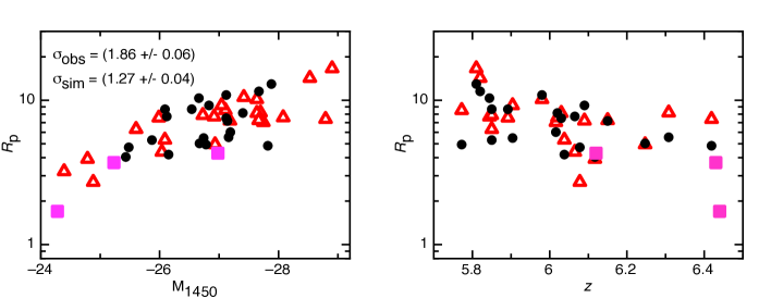
Figure 1: Measured sizes $R_{\rm p}$ plotted against $M_{\rm 1450}$ (Left) and $z$ (Right) respectively, for observed (black dots) and simulated (triangles) near-zones. Measured near-zone sizes are also plotted for CFHQS J$1509-1749$, CFFQS J$2329-0301$ and CFHQS J$0210-0456$ (squares). The simulated data has been computed at the best fit in $\alpha_{0}$ and $\alpha_{1}$ (see text for details).

Fan et al. (2006) found a striking relation between near-zone size and redshift, which they quantify using the expression

$$R_{\rm p}=R_{\rm cor}+A\times(z-6).$$ (1)

Here the near-zone size, $R_{\rm cor}$, has been corrected for luminosity according to the relation

$$R_{\rm corr}=R_{27}\times 10^{-0.4(27+M_{\rm 1450})/B},$$ (2)

where $B=3$ and $R_{27}$ is the mean size of a near-zone at $z=6$ around a quasar of $M_{\rm 1450}=-27$. The value of $B=3$ (which is roughly consistent with observations, Carilli et al., 2010) is motivated by the evolution of an HII region (Haiman, 2002)

$$R_{\rm p} = 4.2f_{\rm HI}^{-1/3}\left(\frac{\dot{N}}{1.9\times 10^{57}\mbox{s}^{-1}}\right)^{1/3}$$ (3)

$$\hskip 28.45274pt\times\left(\frac{t}{10^{7}\mbox{yr}}\right)^{1/3}\left(\frac{1+z}{7}\right)^{-1}\mbox{Mpc},$$

where $f_{\rm HI}$ is the fraction of hydrogen that is neutral, $\dot{N}$ is the rate of ionizing photons produced by the quasar, and $t$ is the quasar age. The size of the near-zones is found to increase by a factor of 2 over the redshift range from $6.4>z>5.7$, from which Fan et al. (2006) inferred the neutral fraction to increase by an order of magnitude over that time.

On the other hand, if the near-zone size is set by resonant absorption in an otherwise ionized IGM rather than by the boundary of an HII region, then its value is instead approximated by the expression

$$R_{\rm p} \sim \frac{3.1}{\Delta_{\rm lim}}\left(\frac{\tau_{\rm lim}}{2.3}\right)^{1/2}\left(\frac{T}{2\times 10^{4}\mbox{K}}\right)^{0.35}\left(\frac{\dot{N}}{1.9\times 10^{57}\mbox{s}^{-1}}\right)^{1/2}$$ (4)

$$\hskip 28.45274pt\times\left(\frac{\alpha^{-1}[\alpha+3]}{3}\right)^{-1/2}\left(\frac{1+z}{7}\right)^{-9/4}\mbox{Mpc},$$

where $\Delta_{\rm lim}$ is the normalised baryon density in the transmitting regions as a fraction of the cosmic mean ($\tau_{\rm lim}=2.3$, corresponding to the 10 per cent transmission), and $T$ is the IGM temperature (Bolton & Haehnelt, 2007b). The parameter $\alpha$ is the EUV spectral index. Equation (4) differs from equation (3) in three important ways. Firstly, if near-zone size is set by resonant absorption then it is not sensitive to the quasar lifetime. Secondly, resonant absorption results in a power-law index describing the dependence of near-zone size on luminosity with a value of $B=2$ rather than $B=3$. Thirdly, the near-zone size is sensitive to $\alpha$, suggesting that near-zone size provides an opportunity to measure this unknown parameter.

The precise definition of near-zone radius suggested by Fan et al. (2006) allows for quantitative comparison with simulations. Wyithe et al. (2008) and Bolton et al. (2010) have modelled near-zones using hydro-dynamical simulations with radiative transfer, combined with a semi-analytic model for the evolving, density dependent ionizing background. The modelling in the latter work is able to produce both the amplitude and evolution of the near-zone sizes, as well as the statistics of absorption lines within the near-zone, and is based on quasars in a highly ionized IGM. In this regime it is equation (4) with $B=2$, rather than equation (3) with $B=3$ that is applicable. This indicates that a varying ionizing background could be responsible for the observed relation, providing an alternative scenario to a strongly evolving neutral fraction. Unfortunately, this scenario implies that the evolution of quasar near-zones cannot necessarily be used to infer an evolution in neutral fraction. Thus, although intriguing, it could be argued that the observed near-zone relation has not yet taught us anything concrete about reionization.

When discussing near-zones most authors have concentrated on the relation between size and redshift, with measured size corrected for luminosity dependence as part of this process. In most cases these studies used the scaling of near-zone in proportion to luminosity to the one third power (e.g. Fan et al., 2006; Carilli et al., 2010). As described above this value is appropriate if the near-zone is expanding into a neutral IGM. On the other hand, a power of one half ($B=2$) is more appropriate if the near-zone corresponds to a radius where resonant absorption in an ionized IGM results in the 10 per cent transmission (Bolton & Haehnelt, 2007a). Thus the correct scaling between near-zone radius and quasar luminosity is uncertain. In this work we therefore treat the power-law index $B$ as a free parameter in a 2-dimensional relation describing near-zone radius as a function of quasar luminosity and redshift. We find that current near-zone data places strong constraints on the value of $B$. Moreover, rather than focus on the interpretation of the parameter $A$ with respect to the end of hydrogen reionization, in this paper we concentrate instead on understanding the implications of the parameters $B$ and $R_{27}$ for the EUV spectral index blueward of the Lyman limit for $z\sim 6$ quasars. We show that the near-zone relation offers a probe of the EUV spectrum of quasars at these early epochs, information that is otherwise concealed by the Lyman-limit absorption, and so has previously only been studied for quasars at redshifts of $z\la 1$ (Telfer et al., 2002).

3 Observed Near-Zone Sample

Carilli et al. (2010) have assembled a sample of 25 $z\sim 6$ quasars which have quality rest-frame UV spectra and redshift measurements (Fan et al., 2006; Jiang et al., 2008). Eight of the sample are detected (Wang et al., 2010) in CO. Another nine have redshifts measured (Kurk et al., 2007; Jiang et al., 2007) from the Mg II line emission. For the other eight objects, Carilli et al. (2010) adopt redshifts from the relevant discovery papers, which are mainly determined with the Ly$\alpha$+NV lines (Fan et al., 2006). The measurements are summarized in Table 1 of Carilli et al. (2010), including the quasar absolute AB magnitude at 1450 Å ($M_{1450}$), quasar redshifts ($z$), and near-zone size ($R_{\rm p}$). Three sources in the original sample (Wang et al., 2010) listed in Table 1 of Carilli et al. (2010), $J0353+0104$, $J1044-0125$, and $J1048+4637$, are broad absorption line quasars (Jiang et al., 2008; Fan et al., 2006), while the source $J1335+3533$ has a lineless (Fan et al., 2006) UV spectrum. We exclude these quasars from our analysis owing to the fundamentally different nature of their intrinsic spectra (Carilli et al., 2010; Fan et al., 2006). Thus the sample consists of 21 $z\sim 6$ quasars which we use to analyse the near-zone relation. Near-zone sizes are plotted in Figure 1 as a function of both absolute magnitude and redshift. Typical measurement errors (Carilli et al., 2010) are 1.2 Mpc, 0.4 Mpc, and 0.1 Mpc in the estimated near-zone size ($R_{\rm p}$) introduced by UV, MgII, and CO-determined redshift uncertainties, respectively. There are clear trends with both luminosity (Carilli et al., 2010) and redshift (Fan et al., 2006; Carilli et al., 2010).

We note that quasar near-zone sizes have also been measured (Willott et al., 2007, 2010) for CFHQS J$1509-1749$, CFFQS J$2329-0301$ and CFHQS J$0210-0456$. Following Carilli et al. (2010) we do not include these near-zones, which are drawn from a different data set, in our analysis. However as may be seen from Figure 1, these near-zones lie on the Carilli et al. (2010) correlation, and we have checked that their addition does not significantly alter our results.

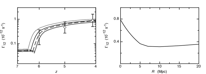
Figure 2: The fiducial model for the ionizing background. Left: The evolution of the ionizing background (Wyithe et al., 2008). The grey curve shows the background in the mean IGM, while the solid, dotted and dashed black curves show the mean and 1-sigma range of ionizing background in the biased regions within $5\,$Mpc of a $10^{13}\,$M_⊙ quasar host halo. The data points show our estimate of the ionizing background at $z=5$ and $z=6$ (error bars represent the 68% range). The point at $z=4$ has been reproduced from Bolton & Haehnelt (2007a). Right: The ionizing background as a function of radius in our fiducial model (for a quasar observed at $z=6$). The ionizing background has been computed as a function of proper time along the trajectory of a photon emitted by the quasar, rather than at the proper time of the quasar.

4 Modelling of Near-Zones

Our near-zone simulations combine a semi-analytical model for the evolving, density dependent photo-ionization rate in the biased regions surrounding quasars, with a radiative transfer implementation, and realistic density distributions drawn from a high resolution cosmological hydrodynamical simulation. These simulations are discussed in detail elsewhere  (Bolton et al., 2010), and their description is not reproduced here. However for completeness we show the evolution of the background photo-ionization rate for our fiducial simulations in the left hand panel of Figure 2. The grey curve shows the photo-ionization rate in the mean IGM, while the solid, dotted and dashed black curves show the mean and 1-sigma range of the photo-ionization rate in the biased regions within $5\,$Mpc of a $10^{13}\,$M_⊙ halo. Importantly, we construct the absorption spectra using an ionizing background computed as a function of proper time along the trajectory of a photon emitted by the quasar, rather than at the proper time of the quasar. This effect is appropriate if considering spectra at the end of the reionization era, when the ionizing background can evolve significantly during the light travel time across a quasar near-zone. The right hand panel of Figure 2 illustrates the background photo-ionization rate as a function of radius in our model (for a quasar observed at $z=6$).

Figure 3: Example synthetic near-zone spectra. In both panels, the dotted curve shows the spectrum after being smoothed to a resolution of 20Å in the observed frame while the vertical dashed line marks the measured near-zone size. This corresponds to the position where the smoothed flux first drops below a transmission of 10 per cent. Top: Quasar at $z=5.8918$ with $M_{1450}=-26.09$. Bottom: Quasar at $z=6.247$ with $M_{1450}=-26.67$.

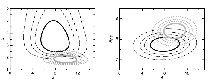
Figure 4: Projections of $\chi^{2}$ for observed (black) and simulated (grey) near-zone sets assuming the fiducial evolving model. We have introduced intrinsic scatter ($\sigma_{\rm obs}=1.86$ Mpc and $\sigma_{\rm sim}=1.27$ Mpc, respectively) so that the reduced $\chi^{2}$ is unity for the best fit model. The contours represent $\Delta\chi^{2}=1$, 2, 3 and 5 relative to the corresponding minimum value of $\chi^{2}$.

For each of the model near-zone sets constructed, the sizes of the simulated near-zones were calculated for a sample of synthetic quasar spectra with the same redshifts and quasar absolute magnitudes as the Carilli et al. (2010) compilation. The synthetic spectra are designed to match the spectral resolution ($R\sim 2500$) and signal to noise of the observational data ($\rm S/N=20$ per $3.5\rm\,\AA$ pixel) as closely as possible. For the fiducial simulations an EUV spectral index of $\alpha=1.5$ (where $dL/d\nu\propto\nu^{-\alpha}$) was assumed to calculate the corresponding ionizing photon rate ($\dot{N}$) from the observed $M_{\rm 1450}$. Additionally, a temperature at mean density of $T=23600^{+5000}_{-6900}$ K has been measured (Bolton et al., 2010) within the near-zone around SDSS J0818+1722. Our fiducial simulations are consistent with this constraint, and we further assume this as the best fit temperature when modelling near-zones throughout our analysis. This level of complexity is important as the near-zone size (Fan et al., 2006) is measured based on the first resolution element where the transmission in the spectrum drops below 10 per cent, meaning that the Ly$\alpha$ forest must be simulated in detail in order for the modelling to be considered reliable. Examples of some of the synthetic quasar spectra used in our analysis are displayed in Figure 3.

5 Near-zone Relation Constraints

As noted in the introduction, the appropriate value of $B$ describing the power-law relation between near-zone size and luminosity is uncertain. Therefore, rather than correct for luminosity by assuming a fixed $B$, and fit equation (1) to determine the evolution of near-zone size with redshift as has been done previously, in our paper we instead model the observed near-zone plane using free parameters to describe both the evolution with redshift ($A$) and the evolution with absolute magnitude ($B$),

$$R_{\rm p}=R_{27}\times 10^{-0.4(27+M_{\rm 1450})/B}+A\times(z-6).$$ (5)

In this section, we use equation (5) to quantify constraints from the near-zone plane at $z\sim 6$.

We find the parameter sets that describe the near-zone plane by fitting equation (5) to both the observed near-zone relation and to our simulated data sets. The black and grey contours in Figure 4 show the resulting projections of $\chi^{2}$ onto the parameter spaces $(A,B)$ and $(A,R_{27})$ for the observed and fiducial simulated near-zones, respectively. When calculating $\chi^{2}$ we introduce intrinsic scatter into equation (5) so that the reduced $\chi^{2}$ of the best fit model is unity. We find a smaller intrinsic scatter ($\sigma_{\rm sim}=1.27\pm 0.04$ Mpc) in the simulated data, indicating that sight-line variation is not responsible for all of the observed scatter ($\sigma_{\rm obs}=1.86\pm 0.06$).

While the simulations reproduce the size evolution with redshift, the luminosity dependence is not well described, with $B\sim 2$ for the simulations (equation 4) but $B\sim 3$ for the observed sample. There are two explanations for this disagreement between the data and fiducial model which we now discuss in turn.

6 Near-zone relation determined by HII regions

Firstly, the observed value of $B=3$ is expected if the quasars were surrounded by HII regions embedded in a neutral IGM (Cen & Haiman, 2000). Naively, this could be interpreted as evidence for a significantly neutral IGM. To test this, we calculate the expected scatter in the near-zone relation for comparison with observation. In contrast to the case for a proximity zone in an optically thin IGM, the size of an HII region depends on the age of the quasar at the time of observation. As a result, there is scatter in the observed size even for fixed redshift and quasar luminosity. We can estimate the scatter due to the age of the quasars by noting that if there is equal probability of observing a quasar at any age during its lifetime, then the probability distribution for the HII region radius at fixed luminosity $L$ and redshift $z$, given a quasar lifetime $t_{\rm max}$, is

$$\left.\frac{dP}{dR_{\rm p}}\right|_{L,z}=\frac{3R_{\rm p}^{2}}{R_{\rm max}^{3}},$$ (6)

where $R_{\rm max}$ is the size reached after $t_{\rm max}$. Given this distribution, the mean is $\langle R_{\rm p}\rangle=3/4\,R_{\rm max}$, and the variance is $\sigma_{R}^{2}\equiv\langle R_{\rm p}^{2}\rangle-\langle R_{\rm p}\rangle^{2}=\langle R_{\rm p}\rangle^{2}/15$. Observationally, since we have $\langle R_{\rm p}\rangle\sim R_{27}\sim 8$ Mpc, the scatter in HII region radius owing to random quasar age is $\sigma_{R}\sim 2$ Mpc. Thus the scatter in observed quasar age accounts for all of the observed scatter ($\sigma_{\rm obs}=1.86\pm 0.06$) in the near-zone sizes. However in the case of HII regions we would also expect additional scatter in the size owing to other quantities like the quasar lifetime and the spectral index (we return to this point below), as well as scatter due to inhomogeneities in the density field and ionization structure along the different quasar sight-lines. In the case of the latter, the sizes of HII regions near the end of reionization (Furlanetto et al., 2004) are thought to vary over the range 1-2 proper Mpc, which would lead to a component of scatter in addition to the $\sim 2\,$Mpc expected from the quasar age. Thus, the total scatter in an HII region generated near-zone relation would be in excess of $\sigma_{R}\sim 3$ Mpc. We therefore infer that although quasar HII regions would lead to a near-zone relation with the appropriate value of $B\sim 3$, the observed relation between near-zone size and magnitude would be too tight in this case. This scatter based constraint would be alleviated if the near-zone sizes corresponded to resonant absorption within an HII region (the scatter would be smaller since the size is independent of lifetime in this case). However, in this alternative case where resonant absorption sets the near-zone size, our modelling suggests that $B\sim 2$ rather than $B\sim 3$ should be observed. As a result, HII regions cannot provide a viable physical explanation for the observational data (see also Maselli et al., 2009).

7 Constraining the EUV spectral index

An alternative scenario to explain this trend is provided by an EUV spectral index which is luminosity dependent, so that at brighter absolute magnitudes the ionizing flux is smaller. To quantify this point, we first note that the observed quantities are the near-zone size and the absolute UV magnitude. Given this UV magnitude, the ionization properties of the surrounding medium are dependent on the ionizing luminosity in photons per second ($\dot{N}$), and the spectral index blueward of the Lyman break. The relation between $\dot{N}$ and $\alpha$ is

$$\dot{N}=\int_{\nu_{\rm Ly}}^{x_{\rm max}\nu_{\rm Ly}}d\nu\frac{L_{\nu_{\rm Ly}}}{h\nu}\left(\frac{\nu}{\nu_{\rm Ly}}\right)^{-\alpha},$$ (7)

where $L_{\nu_{\rm Ly}}$ is the luminosity at the Lyman limit $\nu_{\rm Ly}$, $h$ is Planck’s constant and $x_{\rm max}$ is the ratio between the frequency where photons cease to contribute to ionization and the Lyman limit (we take $x_{\rm max}=100$, though this choice does not affect our results). To estimate the value of $\dot{N}$ for the quasars in the Carilli et al. (2010) sample, the observed $M_{1450}$ has previously (Bolton et al., 2010) been combined with an assumed a spectral index of $\alpha=1.5$. Our approach to investigate whether a variable spectral index is able to explain the discrepancy in $B$ is therefore to modify the value of absolute magnitude that corresponds to the ionization rate at the near-zone radius measured in the simulations. This allows us to investigate the near-zone relations that result from a range of spectral indicies without re-calculating the radiative transfer simulations. Beginning with equation (4) and equation (7) and assuming a spectrum of the form

$$L_{\nu}(\nu)=L_{1450}\left(\frac{\nu_{1050}}{\nu_{1450}}\right)^{-0.5}\left(\frac{\nu_{\rm Ly}}{\nu_{1050}}\right)^{-\alpha}\left(\frac{\nu}{\nu_{\rm Ly}}\right)^{-\alpha},$$ (8)

we adjust the absolute magnitude corresponding to the model quasars (at fixed near-zone radius) for a variation in spectral index using

$$M_{\rm 1450} = M_{\rm 1450,1.5}-2.5\log_{10}\left(\left(\frac{\nu_{912}}{\nu_{1050}}\right)^{\alpha-1.5}\frac{\alpha+3}{4.5}\right.$$ (9)

$$\times\left.\frac{1-x_{\rm max}^{-4.5}}{1-x_{\rm max}^{-(\alpha+3)}}\left(1.71-0.86\alpha+0.33\alpha^{2}-0.05\alpha^{3}\right)^{-0.7}\right),$$

where $M_{\rm b,1.5}$ is the observed absolute magnitude used in the fiducial model. Here we note that simulations performed with $\alpha=0.5$, $\alpha=1.0$, $\alpha=1.5$, $\alpha=2.0$, and $\alpha=2.5$ yield near-zone temperatures of $T\sim 2.81\times 10^{4}$K, $T\sim 2.34\times 10^{4}$K , $T\sim 2.06\times 10^{4}$K , $T\sim 1.89\times 10^{4}$K and $T\sim 1.76\times 10^{4}$K respectively. These values are fit (to within 1%) by

$$T=35400-17700\alpha+6757.1\alpha^{2}-1000\alpha^{3}.$$ (10)

This dependence contributes the last product in equation (9).

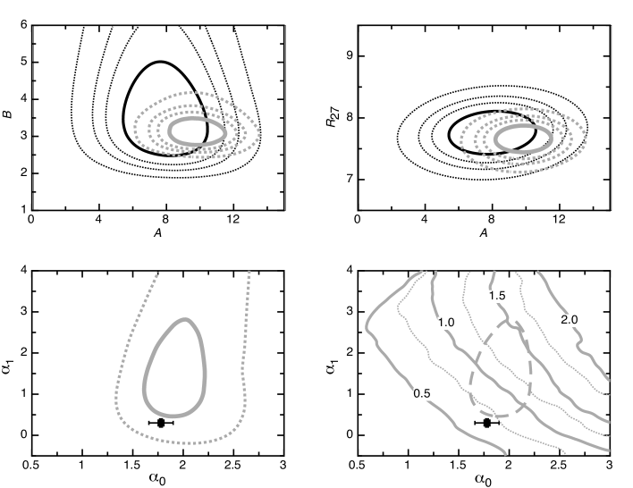
Figure 5: Upper panels: Projections of $\chi^{2}$ for observed (black) and simulated (grey) near-zone sets for the best fit simulations (in $\alpha_{0}$ and $\alpha_{1}$) assuming the fiducial evolving ionizing background. We have introduced intrinsic scatter so that the reduced $\chi^{2}$ is unity for the best fit model. The contours represent $\Delta\chi^{2}=1$, 2, 3 and 5 relative to the corresponding minimum value of $\chi^{2}$. Lower left panel: Contours of likelihood for the values of $\alpha_{0}$ and $\alpha_{1}$ (at 60% and 10% of the peak likelihood). Lower right panel: Contours of scatter in spectral index $\alpha$. The point with error-bars shows the corresponding parameters measured (Telfer et al., 2002) at low redshift.

To quantify the possible dependence of spectral index on luminosity we parametrize the value of $\alpha$ as a function of $M_{\rm 1450}$ using

$$\alpha=\alpha_{0}-\alpha_{1}(M^{\prime}_{\rm 1450}+27),$$ (11)

where $\alpha_{0}$ represents the mean spectral slope of quasars with $M_{1450}=-27$ and $\alpha_{1}=\frac{d\alpha}{dM_{\rm 1450}}$ describes the variation of spectral index with magnitude. Note that since $\alpha$ is a function of $M_{1450}$, we evaluate it not at the observed $M_{1450}$, but instead use an absolute magnitude $M^{\prime}_{1450}$ that is adjusted to account for the average index $\alpha_{0}$ at $M_{1450}=-27$,

$$M^{\prime}_{\rm 1450} = M_{\rm 1450,1.5}-2.5\log_{10}\left(\left(\frac{\nu_{912}}{\nu_{1050}}\right)^{\alpha_{0}-1.5}\frac{\alpha_{0}+3}{4.5}\right.$$ (12)

$$\times\left.\frac{1-x_{\rm max}^{-4.5}}{1-x_{\rm max}^{-(\alpha_{0}+3)}}\left(1.71-0.86\alpha_{0}+0.33\alpha_{0}^{2}-0.05\alpha_{0}^{3}\right)^{-0.7}\right).$$

We use these equations to constrain the likelihood of parameter combinations $(\alpha_{0},\alpha_{1})$ through convolution of the resulting joint probability distribution for the parameters $A$, $B$ and $R_{27}$ that describe simulated near-zone relations, with the corresponding relation for the observations

$$\mathcal{L}_{\alpha_{0},\alpha_{1}}\propto\int dA\,dB\,dR_{27}\frac{d^{3}P_{\rm obs}}{dA\,dB\,dR_{27}}\left.\frac{d^{3}P_{\rm sim}}{dA\,dB\,dR_{27}}\right|_{\alpha_{0},\alpha_{1}}\mathcal{L}_{\sigma_{\rm sim}},$$

where

$$\frac{d^{3}P_{\rm obs}}{dA\,dB\,dR_{27}}\propto e^{-\frac{\chi_{\rm obs}^{2}(A,B,R_{27})}{2}},$$

and

$$\frac{d^{3}P_{\rm sim}}{dA\,dB\,dR_{27}}\propto e^{-\frac{\chi_{\rm sim}^{2}(A,B,R_{27})}{2}}.$$ (13)

Here we have assumed flat prior probability distributions for each of the parameters $A$, $B$ and $R_{27}$. As part of this procedure we calculate the intrinsic scatter for each set of parameters $(\alpha_{0},\alpha_{1})$, and impose the condition that this scatter be smaller than the observed scatter by weighting the calculated likelihood with

$$\mathcal{L}_{\sigma_{\rm sim}} \propto e^{\frac{-(\sigma_{\rm obs}-\sigma_{\rm sim})^{2}}{2(0.06^{2})}},\hskip 8.53581pt\mbox{where}\hskip 8.53581pt\sigma_{\rm obs}<\sigma_{\rm sim}$$ (14)

$$\propto 1\hskip 8.53581pt\mbox{otherwise.}$$

Here the value of 0.06 dex represents the uncertainty in $\sigma_{\rm obs}$.

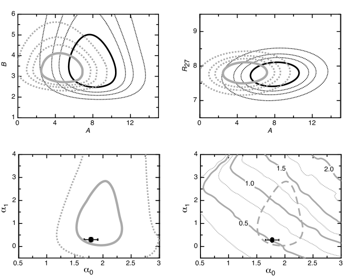
Figure 6: Upper panels: Projections of $\chi^{2}$ for observed (black) and simulated (grey) near-zone sets for the best fit simulations (in $\alpha_{0}$ and $\alpha_{1}$) assuming the non-evolving ionizing background. We have introduced intrinsic scatter so that the reduced $\chi^{2}$ is unity for the best fit model. The contours represent $\Delta\chi^{2}=1$, 2, 3 and 5 relative to the corresponding minimum value for $\chi^{2}$. Lower left panel: Contours of likelihood for the values of $\alpha_{0}$ and $\alpha_{1}$ (at 60% and 10% of the peak likelihood). Lower right panel: Contours of scatter in spectral index $\alpha$. The point with error-bars shows the corresponding parameters measured (Telfer et al., 2002) at low redshift.

Contours of likelihood for the values of $\alpha_{0}$ and $\alpha_{1}$ based on our fiducial model are plotted in the lower left panel of Figure 5. We find that the preferred value of $\alpha_{0}$ is smaller than the assumed $\alpha=1.5$. In addition, since the fiducial simulations under-predict $B$ (Figure 4), the value of $\alpha_{1}$ is found to be greater than zero with high confidence, so that more luminous quasars have softer spectra. This is consistent with the results of Strateva et al. (2005), who found that brighter quasars are relatively less luminous in the X-ray, and is also expected from theoretical modeling of the quasar spectrum (Wandel & Petrosian, 1988).

The corresponding contours (grey curves) of $\Delta\chi^{2}$ in the parameter spaces $(A,B)$ and $(A,R_{27})$ for the simulated near-zone relations computed using the most likely values of $\alpha_{0}$ and $\alpha_{1}$ are shown in the upper panels of Figure 5, along with contours for the observed near-zone sample (black curves). The best fit simulations reproduce the observed values of average size $R_{27}$ and index $B$. The parameter $A$, which is sensitive to the evolution of the ionizing background, is also consistent with observations (Fan et al., 2006; Bolton & Haehnelt, 2007b). The near-zone sizes for the best fit model are plotted in Figure 1 (triangles).

7.1 Intrinsic scatter in the spectral index

As mentioned previously in section 5, the intrinsic scatter in the simulated near-zones ($\sigma_{\rm sim}=1.25$ for the best fit model) is smaller than the scatter $\sigma_{\rm obs}=1.86$ in the observed near-zone relation. Since the numerical simulations already include line-of-sight density variations in the IGM, the missing scatter

$$\Delta R_{\rm p}=\sqrt{\sigma_{\rm obs}^{2}-\sigma_{\rm sim}^{2}}$$ (15)

could be provided by scatter in the spectral index among individual quasars, which is known to be significant at lower redshift (Telfer et al., 2002). Using the relation for the missing scatter in $R_{\rm p}$ we obtain the magnitude of scatter in the spectral index that is necessary to simulate the observed near-zone scatter

$$\Delta\alpha=\frac{d\alpha}{dM}\frac{dM}{dR}\Delta R=\alpha\frac{B}{R_{27}}\sqrt{\sigma_{\rm obs}^{2}-\sigma_{\rm sim}^{2}}.$$ (16)

Contours of this scatter are shown in the right hand panel of Figure 5. Values for scatter in spectral index ranging between $\Delta\alpha\sim 0.75$ and $\Delta\alpha\sim 1.25$ correspond to the range of parameters $\alpha_{0}$ and $\alpha_{1}$ which lead to models for the near-zone relation that are in good agreement with the data.

7.2 Constant ionizing background models

Our simulations of quasar near-zones assume a semi-analytic model for the ionizing background (see Wyithe et al., 2008). It is therefore important to ask whether the results in this paper pertaining to the dependence of near-zone size on luminosity (i.e. the constraints on $B$), and the resulting conclusions regarding the quasar spectral index $\alpha$ are sensitive to this model. To address this issue we have repeated our modelling of quasar near-zones assuming an ionizing background that is independent of redshift. We first take the $z=6$ value from our fiducial model; Figure 6 shows contours describing the resulting constraints (grey curves). The results are very similar to the fiducial case, with the exception of $A$, which shows that the redshift evolution of near-zone size in the constant background model is smaller than observed. This is consistent with the previous inference that the trend of near-zone size with redshift is being driven by the rising intensity of the ionizing background (Wyithe et al., 2008) at $z\sim 6$. We have also tested sensitivity to the ionizing background amplitude by repeating our analysis for 16 different values ranging between 1/100 and $\sqrt{10}$ times the fiducial model. In the left panel of Figure 7 we show the resulting range for $\alpha_{0}$ as a function of the background photoionization rate $\Gamma_{12}=\Gamma_{\rm HI}/10^{-12}\rm\,s^{-1}$. This figure illustrates that results for $\alpha$ depend on the assumed value of $\Gamma_{12}$. As a result, we next constrain $\Gamma_{12}$ following the work of Bolton & Haehnelt (2007b).

7.2.1 The Ionizing Background at $z=6$

$z$	$\mathcal{T}$	$\sigma_{\mathcal{T}}$
4.92	0.1276	0.0011
4.95	0.1139	0.0022
4.98	0.1002	0.0050
5.01	0.1268	0.0117
5.04	0.1567	0.0073
5.06	0.1765	0.0190
5.06	0.1285	0.0042
5.06	0.1509	0.0224
5.07	0.0751	0.0011
5.08	0.0530	0.0025
5.10	0.0898	0.0020
5.11	0.1650	0.0030
5.13	0.1293	0.0064
5.13	0.1243	0.0050
5.90	0.0108	0.0033
5.93	0.0125	0.0022
5.95	0.0038	0.0005
5.95	0.0060	0.0010
6.08	-0.0071	0.0020
6.10	0.0012	0.0010
6.10	0.0051	0.0005
6.25	0.0015	0.0005

Table 1: Table of transmissions $\mathcal{T}$ and uncertainty $\sigma_{\mathcal{T}}$ in $\Delta z=0.1$ regions from Fan et al. (2006).

Figure 7: Left Panel: The best-fit value for $\alpha_{0}$ as a function of $\Gamma_{12}$ (solid curve), together with the 68% range (dashed curves). Central Panel: The joint probability distribution for $\Gamma_{12}$ and $\alpha_{0}$. The prior probability for $\Gamma_{12}$ is assumed to be flat in the logarithm ($dP_{\rm prior}/d\Gamma_{12}\propto 1/\Gamma_{12}$). Right Panel: The joint probability distribution for $\alpha_{0}$ and $\alpha_{1}$. In the central and right panels the contours represent levels that are at 60% and 10% of the peak likelihood. The final estimate for the EUV spectral index is $\alpha_{0}=1.3^{+0.4}_{-0.3}$.

Fan et al. (2006) present eight values of transmission $\mathcal{T}$ (with uncertainty $\sigma_{\mathcal{T}}$) measured in redshift intervals of $\Delta z=0.1$ centred on redshifts in the range $5.9\leq z\leq 6.25$, and 14 values centred in the redshift range $4.9\leq z\leq 5.15$. These values are listed in Table 1. From these values we calculate the mean value of transmission $\langle\mathcal{T}\rangle=0.004\pm 0.002$ and $\langle\mathcal{T}\rangle=0.12\pm 0.01$ respectively. To estimate this uncertainty we have calculated the standard error on the mean transmission via a bootstrap analysis which includes the uncertainties on individual parameters. The values of $\langle\mathcal{T}\rangle=0.004$ and $\langle\mathcal{T}\rangle=0.12$ are consistent with the values quoted previously (Bolton & Haehnelt, 2007a) at $z=6$ and $z=5$ respectively, although note that this study uses slightly wider redshift bins and does not use the independent data of Songaila (2004). However our estimates of the uncertainty are smaller, particularly at $z=6$ where the previously quoted error (Bolton & Haehnelt, 2007a) is a factor of $\sim 2$ larger. This difference can be attributed to the fact that rather than estimate the standard error on the mean transmission, Bolton & Haehnelt (2007a) used an inter-quartile range as an estimate for the error on the transmission values along various lines of sight.

To estimate the corresponding background photo-ionization rate we next combine previously published (Bolton & Haehnelt, 2007a) data with a Monte-Carlo method. We first determine the resulting distribution of effective optical depths from our transmission estimates, finding values of $\tau_{\rm eff}=5.5_{-0.4}^{+0.6}$ and $\tau_{\rm eff}=2.1_{-0.07}^{+0.08}$ at $z=6$ and $z=5$ respectively. Here and below we have quoted the median and the 68% range. We note that the value of $\tau_{\rm eff}$ is not defined in the small number of cases where the Monte-Carlo trial value of $\mathcal{T}$ is negative. In such cases we set $\mathcal{T}=10^{-6}$ and note that our results are insensitive to the exact value provided it is well below the observational limits in the Gunn-Peterson troughs. Given the distribution of effective optical depths, we determine the corresponding probability distribution for the normalized photoionization rate $\Gamma_{12}=\Gamma_{\rm HI}/10^{-12}\rm\,s^{-1}$. To estimate the uncertainties we have utilized scaling relations derived from hydrodynamical simulations (see Table 4 of Bolton & Haehnelt, 2007a) for $\Gamma_{12}$, as functions of $\tau_{\rm eff}$, the IGM temperature [which we take to be $\log_{10}{(T/10^{4}\mbox{K})}=0\pm 0.3$], and the slope of the temperature density relation. We also utilize scaling relations as a function of the cosmological parameters.

At $z=5$ we find $\Gamma_{12}=0.47_{-0.2}^{+0.3}$, while at $z=6$ we obtain $\Gamma_{12}=0.18_{-0.09}^{+0.18}$. We note that the smaller uncertainty in $\tau_{\rm eff}$ relative to the previous estimate  (Bolton & Haehnelt, 2007a) allows us to quote a probability density for the measured ionizing background (with a non-zero value preferred at 2$\sigma$) rather than an upper limit. The revised estimates of the ionizing background at $z=5$ and $z=6$ are presented in Figure 2.

7.2.2 Joint Probability for $\Gamma_{12}$ and $\alpha_{0}$

We use the constraints for $\Gamma_{12}$, together with the likelihoods for $\alpha_{0}$ and $\alpha_{1}$ as a function of $\Gamma_{12}$, to generate a joint probability distribution for $\Gamma_{12}$ and $\alpha_{0}$ (central panel of Figure 7). Similarly, we obtain the joint probability for $\alpha_{0}$ and $\alpha_{1}$ (right hand panel of Figure 7). This procedure yields an estimate of $\alpha_{0}=1.3^{+0.4}_{-0.3}$. This constraint represents the primary measurement of our paper.

7.3 Comparison with spectral index at low redshift

Telfer et al. (2002) measured the UV spectral index for quasars at $z\sim 1-2$. By analysing the composite spectrum they found a mean value of $\langle\alpha\rangle=1.76\pm 0.12$. Telfer et al. (2002) also measured $\alpha$ for a sub-sample of individual quasars, allowing them to estimate the variation $\alpha_{1}=0.3\pm 0.1$ with luminosity, as well as the intrinsic scatter $\Delta\alpha=0.76$. These estimates are plotted alongside our model constraints in Figure 5-8. We find that the parameter combination $\alpha_{0}=1.76\pm 0.12$ and $\alpha_{1}=0.3\pm 0.1$ is consistent with our inference for these parameters at $z\sim 6$. Moreover, we find that our inferred scatter in $\alpha$ at $z\sim 6$ agrees well with the $\Delta\alpha=0.76$ found by Telfer et al. (2002). Thus, assuming our fiducial model of the ionizing background, there is no evidence for evolution in the EUV slope of quasars with redshift out to $z\sim 6$.

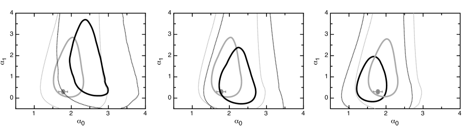
Figure 8: Figure showing the systematic uncertainties on the joint probability distribution for $\alpha_{0}$ and $\alpha_{1}$. Left panel: The dark contours show constraints that have been computed based on a model with $\alpha=0.5$. Central panel: The dark contours show the constraints in a case where the continuum has been deliberately placed at a level that is 5% too low. Right panel: The dark contours show the constraints in a case where where self-shielded absorbers have been added to regions with density contrast $\Delta>16$. In each case the model assumes an unevolving ionizing background, for which the light contours in each panel show the constraints. The contours represent levels that are at 60% and 10% of the peak likelihood respectively.

8 Uncertainties

In addition to those already discussed, we have checked several other sources of uncertainty. Specifically, we have recalculated our constraints including the assumption of a fiducial model with $\alpha=0.5$ rather than $\alpha=1.5$, a model where the quasar continuum has been placed systematically high by 5% on the data, and a model that includes an approximate treatment of Lyman limit systems. Each of these effects is found to have a relatively small effect on the derived parameters for the spectral index relative to the quoted uncertainty, as detailed below.

8.1 Near-zone temperature

There is an uncertainty in the absolute temperature of the IGM within the quasar near-zone, as well as scatter in the temperature from one near-zone to another. These uncertainties will impact on our constraints for the EUV spectral index. Firstly, any scatter in temperature among different near-zones will contribute to scatter in the observed near-zone sizes. However this scatter will be degenerate with scatter in the spectral index ($\Delta\alpha$). Thus the potential presence of scatter in temperature does not introduce uncertainty into our estimated mean value of $\alpha_{0}$ or $\alpha_{1}$. However, it does imply that our quoted $\Delta\alpha$ should be considered an upper limit.

On the other hand, uncertainty in the absolute value of the temperature within the near-zones could introduce a more serious error. The temperature of the IGM in the quasar near-zone has two independent contributions which add linearly, and hence the near-zone temperature has two components of uncertainty. Firstly, the mean IGM has an uncertainty in temperature resulting from heating during hydrogen reionization. This component of uncertainty in the temperature due to hydrogen reionization is already included (Bolton & Haehnelt, 2007a) in the calculation of the ionizing background.

However in addition the reionization of HeII by the quasar may heat the IGM in the near-zone to well above this mean IGM temperature (Bolton et al., 2009). In our modelling we have assumed a temperature (Bolton et al., 2010) that is consistent with observations of a single $z\sim 6$ quasar (SDSS J0818+1722), and that the quasar is responsible for reionization of HeII within the near-zone. This latter assumption means the temperature increase from HeII reionization by the quasar is directly related to the spectral hardness of the quasar, and hence to $\alpha$, which is the quantity we are trying to measure. As a result, the assumption of an incorrect temperature could bias the inferred value of $\alpha$ in our analysis. A hardening of the spectral index leads both to higher temperatures within the near-zone and to an enhanced photo-ionization rate. By assuming a fixed temperature for all modelling our analysis would include only the latter enhancement, whereas both ionization and temperature influence the optical depth. We have therefore accounted for this effect via the scaling in equation (9) based on a calibration of near-zone temperature with spectral index estimated from additional radiative transfer simulations. Furthermore, to check the importance of the temperature effects, and at the same time check that our assumed fiducial value of $\alpha$ does not influence the results, we have repeated the constraints on $\alpha_{0}$ and $\alpha_{1}$ based on the fiducial unevolving ionizing background using a simulated quasar with a value of $\alpha=0.5$ (and correspondingly hotter temperature). As shown in the left panel of Figure 8, we find that the assumed fiducial $\alpha$ (and corresponding fiducial temperature) does not strongly influence the constraints.

8.2 Continuum placement

In addition to errors in the redshifts of the quasars, uncertainty in continuum placement may also lead to an error in the near-zone radius $R_{\rm p}$. This error corresponds to an uncertainty (Fan et al., 2006) of $\Delta\tau\sim 0.05$, or equivalently to a relative uncertainty in the transmission of $\Delta\mathcal{T}/\mathcal{T}\sim 5\%$. At the near-zone radius $\mathcal{T}=10\%$, so that the uncertainty in transmission is $\Delta\mathcal{T}\sim 0.005$. Inspection of Figure 3 in Carilli et al. (2010) shows that when averaged over the near-zone sample, the gradient of transmission with radius is $d\mathcal{T}/dR_{\rm p}\sim 0.05$ Mpc^-1. Hence the uncertainty in the near-zone radius that is introduced by the uncertainty in continuum placement is $\Delta R_{\rm p}\sim dR_{\rm p}/d\mathcal{T}\Delta\mathcal{T}\sim 0.1$Mpc. Thus, continuum placement is sub-dominant in terms of contribution to the uncertainty in near-zone size. We note that the uncertainty could be larger for individual quasars. However this would introduce additional scatter into the near-zone relation which would be degenerate with the other sources of scatter. To check this conclusion we have again repeated the constraints on $\alpha_{0}$ and $\alpha_{1}$ based on an unevolving ionizing background using simulated quasars for which the continuum has been systematically placed 5 per cent too low. As shown in the central panel of Figure 8, we find that the continuum placement has a systematic effect on near-zone size and hence $\alpha_{0}$. However the shift is much smaller than the statistical uncertainty. We thus conclude that our results are robust to a systematic uncertainty in the continuum at this level.

8.3 Lyman limit systems

Finally, a potential shortcoming of our modelling is the assumption that the IGM is optically thin, which results in the absence of absorbers that are self-shielded with respect to the ionizing background. To address this we have tested the sensitivity of near-zone size by adding a population of self-shielded Ly-limit systems. We achieve this by setting all gas with density contrast $\Delta>16$ (corresponding to the density contrast of a clump that will self shield if immersed in our fiducial ionizing background, Furlanetto & Oh, 2005) to be neutral prior to the quasar turning on (Bolton & Haehnelt, 2007a). We find that their inclusion does not alter the predicted distribution of near-zone sizes in most cases, and that as shown in Figure 8, the presence of self-shielded systems should not significantly modify our measurement of $\alpha_{0}$ relative to other uncertainties.

A related question concerns an alternative explanation for the observed $B=3$ due to an enhanced number density of absorbing systems in the biased environments surrounding luminous quasars. Such an enhancement could preferentially retard the observed near-zone sizes, leading to an increase in near-zone size with luminosity that is slower than expected in the optically thin regime. However we have previously (Bolton & Haehnelt, 2007a) investigated the dependence of near-zone size on quasar host-halo mass, finding a negligible effect. This is because the absorbers that set the near-zone size are located between 30 and 100 co-moving Mpc from the quasar. Thus, the environmental dependence of absorber abundance is unlikely to explain the observed $B=3$.

9 conclusion

The discovery of a strong correlation of the sizes of near-zones around high redshift quasars and their redshift in the range $5.7\la z\la 6.4$ (Fan et al., 2006; Carilli et al., 2010) has prompted a series of studies aimed at understanding its implications for the tail end of reionization (Fan et al., 2006; Bolton & Haehnelt, 2007a; Wyithe et al., 2008; Bolton et al., 2010; Carilli et al., 2010). In this paper we have noted that the amplitude of the near-zone radius relation is sensitive to the assumed EUV spectral index of the quasar. We therefore performed a large suite of numerical simulations of the near-zone spectra using radiative transfer through a hydro-dynamical model of the IGM in the quasar environment, and find that the observed near-zone relation can be used to constrain the UV spectral index of $z\sim 6$ quasars. We find that the typical value of spectral index for luminous quasars at $z\sim 6$ is $\alpha=1.3^{+0.4}_{-0.3}$ (for a specific luminosity of the form $L_{\nu}\propto\nu^{-\alpha}$), where the uncertainty includes both the statistical uncertainty in the near-zone relation as well as uncertainty in the ionizing background. Based on comparison of the scatter in our simulations and the scatter in the observed near-zone relation we infer that the scatter in the spectral index is $\Delta\alpha\sim 0.75-1.25$.

Carilli et al. (2010) noted that the data are consistent with near-zone sizes that scale with quasar luminosity as $R_{\rm p}\propto L^{1/B}$, where $B=3$, and that the scatter in the near-zone radius–redshift relation is reduced if this scaling is applied. However as pointed out by Bolton & Haehnelt (2007a), the value of the power-law index $B$ describing the scaling of near-zone radius with luminosity that is physically appropriate depends on whether near-zone sizes are set by HII region boundaries ($B=3$) or resonant absorption in an ionized IGM ($B=2$). Motivated by the possibility of using this second parameter in the near-zone relation to gain a better understanding of its meaning, in this paper we jointly fit the available observations for variation of near-zone size with both redshift and luminosity. From this analysis we find that the observations have an index of $B\sim 3$, with an uncertainty that excludes a value of $B=2$ with high confidence. In contrast to the observations, we find that our fiducial numerical simulations predict a value of $B=2$.

We have discussed two possibilities for this difference. Firstly our simulations are conducted in a highly ionized IGM. It is possible that although these simulations are able to describe the size and evolution of the near-zones (Bolton et al., 2010), they do not represent physical conditions of the IGM at $z\sim 6$, which could instead contain hydrogen that is significantly neutral as previously argued in Wyithe & Loeb (2004) and Wyithe et al. (2005). Although this would lead to the observed $B=3$, we do not believe that this is the case because the observed relation is too tight to be explained by HII regions, the sizes of which contain a range of additional sources of scatter. Instead, we argue that the observed value of $B\sim 3$ is evidence for a UV spectral index that varies with absolute magnitude in the high redshift quasar sample, becoming softer at higher luminosity. This finding is in agreement with theoretical modeling of quasar spectra (Wandel & Petrosian, 1988).

The results of this paper provide the first constraints on the properties of the EUV spectral index of the highest redshift quasars, which are not observable owing to absorption blueward of the Lyman limit. The values we find are in agreement with direct observations at low redshift, and therefore indicate that there is no evidence for evolution in the EUV properties of quasars over most of cosmic time. The new constraints will aid all studies of reionization involving high redshift quasars, which have previously relied on an assumed value of the mean EUV spectral index measured at lower redshift.

References

- Bolton et al. (2010) Bolton J. S., Becker G. D., Wyithe J. S. B., Haehnelt M. G., Sargent W. L. W., 2010, ArXiv e-prints, 10013415
- Bolton & Haehnelt (2007a) Bolton J. S., Haehnelt M. G., 2007a, Month. Notic. R. Astron. Soc., 374, 493
- Bolton & Haehnelt (2007b) Bolton J. S., Haehnelt M. G., 2007b, Month. Notic. R. Astron. Soc., 382, 325
- Bolton et al. (2009) Bolton J. S., Oh S. P., Furlanetto S. R., 2009, Month. Notic. R. Astron. Soc., 395, 736
- Brandt et al. (2002) Brandt W. N., Schneider D. P., Fan X., Strauss M. A., Gunn J. E., Richards G. T., Anderson S. F., Vanden Berk D. E., Bahcall N. A., Brinkmann J., Brunner R., Chen B., Hennessy G. S., Lamb D. Q., Voges W., York D. G., 2002, Astroph. J. L., 569, L5
- Carilli et al. (2010) Carilli C. L., Wang R., Fan X., Walter F., Kurk J., Riechers D., Wagg J., Hennawi J., Jiang L., Menten K. M., Bertoldi F., Strauss M. A., Cox P., 2010, ArXiv e-prints, 10030016
- Cen & Haiman (2000) Cen R., Haiman Z., 2000, Astroph. J. L., 542, L75
- Dietrich et al. (2003) Dietrich M., Hamann F., Shields J. C., Constantin A., Heidt J., Jäger K., Vestergaard M., Wagner S. J., 2003, Astroph. J., 589, 722
- Fan (2006) Fan X., 2006, New Astronomy Review, 50, 665
- Fan et al. (2006) Fan X., Strauss M. A., Becker R. H., White R. L., Gunn J. E., Knapp G. R., Richards G. T., Schneider D. P., Brinkmann J., Fukugita M., 2006, Astron. J., 132, 117
- Fan et al. (2006) Fan X., Strauss M. A., Richards G. T., Hennawi J. F., Becker R. H., White R. L., Diamond-Stanic A. M., Donley J. L. e. a., 2006, Astron. J., 131, 1203
- Furlanetto & Oh (2005) Furlanetto S. R., Oh S. P., 2005, Month. Notic. R. Astron. Soc., 363, 1031
- Furlanetto et al. (2004) Furlanetto S. R., Zaldarriaga M., Hernquist L., 2004, Astroph. J., 613, 1
- Haiman (2002) Haiman Z., 2002, Astroph. J. L., 576, L1
- Hamann & Ferland (1993) Hamann F., Ferland G., 1993, Astroph. J., 418, 11
- Jiang et al. (2008) Jiang L., Fan X., Annis J., Becker R. H., White R. L., Chiu K., Lin H., Lupton R. H., Richards G. T., Strauss M. A., Jester S., Schneider D. P., 2008, Astron. J., 135, 1057
- Jiang et al. (2010) Jiang L., Fan X., Brandt W. N., Carilli C. L., Egami E., Hines D. C., Kurk J. D., Richards G. T., Shen Y., Strauss M. A., Vestergaard M., Walter F., 2010, Nature, 464, 380
- Jiang et al. (2007) Jiang L., Fan X., Vestergaard M., Kurk J. D., Walter F., Kelly B. C., Strauss M. A., 2007, Astron. J., 134, 1150
- Komatsu et al. (2009) Komatsu E., Dunkley J., Nolta M. R., Bennett C. L., Gold B., Hinshaw G., Jarosik N., Larson D., Limon M., Page L., Spergel D. N., Halpern M., Hill R. S., Kogut A., Meyer S. S., Tucker G. S., Weiland J. L., Wollack E., Wright E. L., 2009, Astroph. J. Suppl. Ser., 180, 330
- Kramer & Haiman (2008) Kramer R. H., Haiman Z., 2008, Month. Notic. R. Astron. Soc., 385, 1561
- Kramer & Haiman (2009) Kramer R. H., Haiman Z., 2009, Month. Notic. R. Astron. Soc., 400, 1493
- Kurk et al. (2007) Kurk J. D., Walter F., Fan X., Jiang L., Riechers D. A., Rix H., Pentericci L., Strauss M. A., Carilli C., Wagner S., 2007, Astroph. J., 669, 32
- Lidz et al. (2007) Lidz A., McQuinn M., Zaldarriaga M., Hernquist L., Dutta S., 2007, Astroph. J., 670, 39
- Maselli et al. (2009) Maselli A., Ferrara A., Gallerani S., 2009, Month. Notic. R. Astron. Soc., 395, 1925
- Maselli et al. (2007) Maselli A., Gallerani S., Ferrara A., Choudhury T. R., 2007, Month. Notic. R. Astron. Soc., 376, L34
- Mesinger et al. (2004) Mesinger A., Haiman Z., Cen R., 2004, Astroph. J., 613, 23
- Pentericci et al. (2003) Pentericci L., Rix H., Prada F., Fan X., Strauss M. A., Schneider D. P., Grebel E. K., Harbeck D., Brinkmann J., Narayanan V. K., 2003, Astron. and Astroph., 410, 75
- Songaila (2004) Songaila A., 2004, Astron. J., 127, 2598
- Srbinovsky & Wyithe (2007) Srbinovsky J. A., Wyithe J. S. B., 2007, Month. Notic. R. Astron. Soc., 374, 627
- Strateva et al. (2005) Strateva I. V., Brandt W. N., Schneider D. P., Vanden Berk D. G., Vignali C., 2005, Astron. J., 130, 387
- Telfer et al. (2002) Telfer R. C., Zheng W., Kriss G. A., Davidsen A. F., 2002, Astroph. J., 565, 773
- Vanden Berk et al. (2001) Vanden Berk D. E., Richards G. T., Bauer A., Strauss M. A., Schneider D. P., Heckman T. M., York D. G., Hall P. B., Fan X., Knapp G. R., et al. 2001, Astron. J., 122, 549
- Vignali et al. (2003) Vignali C., Brandt W. N., Schneider D. P., Anderson S. F., Fan X., Gunn J. E., Kaspi S., Richards G. T., Strauss M. A., 2003, Astron. J., 125, 2876
- Wandel & Petrosian (1988) Wandel A., Petrosian V., 1988, Astroph. J. L., 329, L11
- Wang et al. (2010) Wang R., Carilli C. L., Neri R., Riechers D. A., Wagg J., Walter F., Bertoldi F., Menten K. M., Omont A., Cox P., Fan X., 2010, ArXiv e-prints
- White et al. (2003) White R. L., Becker R. H., Fan X., Strauss M. A., 2003, Astron. J., 126, 1
- Willott et al. (2010) Willott C. J., Albert L., Arzoumanian D., Bergeron J., Crampton D., Delorme P., Hutchings J. B., Omont A., Reyle C., Schade D., 2010, ArXiv e-prints
- Willott et al. (2007) Willott C. J., Delorme P., Omont A., Bergeron J., Delfosse X., Forveille T., Albert L., Reylé C., Hill G. J., Gully-Santiago M., Vinten P., Crampton D., Hutchings J. B., Schade D., Simard L., Sawicki M., Beelen A., Cox P., 2007, Astron. J., 134, 2435
- Willott et al. (2009) Willott C. J., Delorme P., Reylé C., Albert L., Bergeron J., Crampton D., Delfosse X., Forveille T., Hutchings J. B., McLure R. J., Omont A., Schade D., 2009, Astron. J., 137, 3541
- Wyithe et al. (2008) Wyithe J. S. B., Bolton J. S., Haehnelt M. G., 2008, Month. Notic. R. Astron. Soc., 383, 691
- Wyithe & Loeb (2004) Wyithe J. S. B., Loeb A., 2004, Nature, 427, 815
- Wyithe et al. (2005) Wyithe J. S. B., Loeb A., Carilli C., 2005, Astroph. J., 628, 575