Quantum phase transitions in coupled two-level atoms in a single-mode cavity

Abstract

The dipole-coupled two-level atoms(qubits) in a single-mode resonant cavity is studied by extended bosonic coherent states. The numerically exact solution is presented. For finite systems, the first-order quantum phase transitions occur at the strong interatomic interaction. Similar to the original Dicke model, this system exhibits a second-order quantum phase transition from the normal to the superradiant phases. Finite-size scaling for several observables, such as the average fidelity susceptibility, the order parameter, and concurrence are performed for different interatomic interactions. The obtained scaling exponents suggest that interatomic interactions do not change the universality class.

I introduction

The coherent emission from underdamped one-dimensional Josephson arrays coupled to a single-mode electromagnetic cavity has been experimentally studiedjjarys . This system resembles that of the Dicke modeldicke , which describes N two-level atoms (qubits) coupled to a cavity field. It has been showndickexy that a modified Dicke Hamiltonian including a dipole-dipole interaction between the junctions can describe the cavity-junction system better than the original Dicke model.

The modified Dicke Hamiltonian is also an extension of effective two-qubit modelatoms . A small number of coupled qubits in a single-mode cavity is also very interesting, because it may be realized in several solid-state systems, such as an ensemble of quantum dots Scheibner , Bose-Einstein condensates Schneble , coupled arrays of optical cavities used to simulate and study the behavior of strongly correlated systemsHartmann , and the superconducting quantum interference device coupled with a nanomechanical resonatorWallraff ; squid .

The original Dicke model without a rotating-wave approximation (RWA) on the large scale was exactly solved by the present authors in the numerically sensechenqh . Most works on the modified Dicke model are limited to the rotating-wave approximation. With the progress of the fabrication, the artificial atoms may interact very strongly with on-chip resonant circuitsWallraff ; squid ; Peropadre ; exp , the rotating-wave approximation can not describe well the strong coupling regimetheory , so the numerically exact solution to the modified Dicke model without rotating-wave approximation is also of considerable significance and highly called for.

Quantum phase transitions (QPTs) in the original Dicke model has attracted considerable attentions recentlyEmary ; Lambert1 ; Lambert2 ; liberti ; vidal ; reslen ; plastina . With the consideration of additional interatomic interactions, one nature question is its effect on the modified Dicke model.

In this paper, we extend our previous exact technique to solve the finite size modified Dicke model where dipole-dipole interaction between the qubits are taken into account. The QPTs are then studied systematically. The paper is organized as follows. In Sec.II, the numerically exact solution to the finite-size modified Dicke model is proposed in detail, and the analytical solution in the thermodynamic limit is also presented. The numerical results for both small and large system size are given in Sec.III, where the characterization of the QPTs also also performed. The brief summary is presented finally in the last section.

II Model Hamiltonian

dipole-coupled $N$ two-level atoms interacting with a single-mode cavityjjarys ; atoms can be described by the following modified Dicke modeldickexy

$$H=\omega a^{+}a+\frac{\Delta}{2}\sum_{i=1}^{N}\sigma_{z}^{i}+\frac{\lambda}{\sqrt{N}}\left(a^{+}+a\right)\sum_{i=1}^{N}\sigma_{x}^{i}+\frac{\Omega}{2N}\sum_{i\neq j}^{N}\left(\sigma_{x}^{i}\sigma_{x}^{j}+\sigma_{y}^{i}\sigma_{y}^{j}\right),$$ (1)

where $a^{+}$ and $a$ are the field annihilation and creation operators, $\Delta$ and $\omega$ are the transition frequency of the qubit and the frequency of the single bosonic mode, $\lambda$ is the coupling constant of the atom and cavity, $\Omega$ is the interacting strength of two two-level atoms, and $\sigma_{k}^{i}(k=x,y,z)$ is the Pauli matrix of the $i$ junction. For convenience, the Hamiltonian can be rewritten in terms of the collective spin operators: $S_{k}=\sum_{i=1}^{N}\sigma_{k}^{i}/2,\;\;(k=x,y,z)$ and $S_{\pm}=S_{x}\pm iS_{y}$

$$H=\omega a^{+}a+\Delta S_{z}+\frac{2\lambda}{\sqrt{N}}\left(a^{+}+a\right)S_{x}+\frac{2\Omega}{N}(\mathbf{S}^{2}-S_{z}^{2}),$$ (2)

Where a constant is neglected. Without atom-cavity coupling, i.e.$\lambda=0,$ we have

$$H_{atoms}=\Delta S_{z}+\frac{2\Omega}{N}(\mathbf{S}^{2}-S_{z}^{2}),$$ (3)

Note that the Dicke state $\{\left|j,m\right\rangle,m=-j,-j+1,...j-1,j\}$ is the eigenstate of $S^{2}$ and $S_{z}$ with the eigenvalues $j(j+1)$ and $m.$ The eigen energy of $H_{atoms}$ is given by

$$E=\Delta m+\frac{2\Omega}{N}(j(j+1)-m^{2}),$$ (4)

The ground-state energy is easily obtained as

$$E_{0}=\left(-\Delta+\frac{2\Omega}{N}\right)j$$

So in the ground-state, we have $j=0$ for $\frac{2\Omega}{N}>\Delta$ and $j=N/2$ otherwise. Actually, Eq. (3) is just the Hamiltonian of the isotropic Lipkin-Meshkov-Glick modelLMG , where QPT is of the first-order, as is clearly shown above.

Next, we use a transformed Hamiltonian with a rotation around an $y$ axis by an angle $\frac{\pi}{2}$ , so $S_{x}\rightarrow S_{z},S_{z}\rightarrow-S_{x}$ the Hamiltonian now reads

$$H^{\prime}=\omega a^{+}a-\frac{\Delta}{2}(S_{+}+S_{-})+\frac{2\lambda}{\sqrt{N}}\left(a^{+}+a\right)S_{z}+\frac{2\Omega}{N}(\mathbf{S}^{2}-S_{x}^{2}),$$ (5)

where $S_{+}$ and $S_{-}$ are the collective spin raising and lowing operators and obey the SU(2) Lie algebra $[S_{+},S_{-}]=2S_{z},[S_{z},S_{\pm}]=\pm S_{\pm}$. Since $[H^{\prime},S^{2}]=0,$ we suppose $S^{2}=j(j+1)$, where the total angular momentum $j=N/2-r$. Due to the interaction between any two-level atoms, similar to the above discussion for $\lambda=0$, we have no reason to set $r=0$, unlike in the Dicke modelchenqh . In the practical calculations for the ground-state, $r$ is regarded as a variational integer number and will be determined by the minimization of the ground-state energy. So the Hilbert space of this algebra is spanned by the Dicke state $\{\left|j,m\right\rangle,m=-j,-j+1,...j-1,j\}$, which is the eigenstate of $S^{2}$ and $S_{z}$ with the eigenvalues $j(j+1)$ and $m$.

The Hilbert space of the total system can be expressed in terms of the basis $\{\left|\varphi_{m}\right\rangle_{b}\bigotimes\left|j,m\right\rangle\}$, where the state of bosons$\left|\varphi_{m}\right\rangle_{b}$ and the integer $j$ are to be determined. A ”natural” basis for bosons is Fock state $\left|l\right\rangle_{b}=[(a^{+})^{l}/\sqrt{l!}]\left|0\right\rangle_{b}$. As in the Dicke model, the bosonic number here is not conserved either, so the bosonic Fock space has infinite dimensions, the standard diagonalization procedure (see, for example, Ref. Emary ) is to apply a truncation procedure considering only a truncated number of bosons. Typically, the convergence is assumed to be achieved if the ground-state energy is determined within a very small relative errors. Within this method, one has to diagonalize very large, sparse Hamiltonian in strong coupling regime and/or in adiabatic regime. Furthermore, the calculation becomes prohibitive for larger system size since the convergence of the ground-state energy is very slow. Interestingly, this problem can be circumvented in the following procedure.

By the displacement transformation $A_{m}=a+g_{m}$ with $g_{m}=2\lambda m/\omega\sqrt{N}$, the Schr$\stackrel{{\scriptstyle..}}{{o}}$ dinger equation can be described in columnar matrix, and its $m$ row reads

$$-\Delta j_{m}^{-}\left|\varphi_{m}\right\rangle_{b}\left|j,m-1\right\rangle-\Delta j_{m}^{+}\left|\varphi_{m}\right\rangle_{b}\left|j,m+1\right\rangle$$ (6)

$$-\frac{2\Omega}{N}j_{m}^{-}j_{m-1}^{-}\left|\varphi_{m}\right\rangle_{b}\left|j,m-2\right\rangle-\frac{2\Omega}{N}j_{m}^{+}j_{m+1}^{+}\left|\varphi_{m}\right\rangle_{b}\left|j,m+2\right\rangle$$

$$+\omega\left(A_{m}^{+}A_{m}-g_{m}^{2}\right)\left|\varphi_{m}\right\rangle_{b}\left|j,m\right\rangle+\frac{2}{\Omega}N\left[j(j+1)-(j_{m-1}^{+}j_{m}^{-}+j_{m+1}^{-}j_{m}^{+})\right]\left|\varphi_{m}\right\rangle_{b}\left|j,m\right\rangle$$

$$= E\left|\varphi_{m}\right\rangle_{b}\left|j,m\right\rangle,$$

where $j_{m}^{\pm}=\frac{1}{2}\sqrt{(j(j+1)-m(m\pm 1)}$. Left multiplying $\{\left\langle n,j\right|\}$ gives a set of equations

$$-\Delta j_{n}^{-}\left|\varphi_{n-1}\right\rangle_{b}-\Delta j_{n}^{+}\left|\varphi_{n+1}\right\rangle_{b}-\frac{2\Omega}{N}j_{n}^{-}j_{n-1}^{-}\left|\varphi_{n-2}\right\rangle_{b}-\frac{2\Omega}{N}j_{n}^{+}j_{n+1}^{+}\left|\varphi_{n+2}\right\rangle_{b}$$

$$+\omega\left(A_{n}^{+}A_{n}-g_{n}^{2}\right)\left|\varphi_{n}\right\rangle_{b}+\frac{2}{\Omega}N\left[j(j+1)-(j_{n-1}^{+}j_{n}^{-}+j_{n+1}^{-}j_{n}^{+})\right]\left|\varphi_{n}\right\rangle_{b}=E\left|\varphi_{n}\right\rangle_{b},$$ (7)

where $n=-j,-j+1,...j$.

Note that the linear term for the bosonic operator $a(a^{+})$ is removed, and a new free bosonic field with operator $A(A^{+})$ appears. In the next step, we naturally choose the basis in terms of this new operator, instead of $a(a^{+})$, by which the bosonic state can be expanded as

$$\left|\varphi_{n}\right\rangle_{b} = \sum_{k=0}^{N_{tr}}c_{n,k}(A_{n}^{+})^{k}\left|0\right\rangle_{A_{n}}$$ (8)

$$= \sum_{k=0}^{N_{tr}}c_{n,k}\frac{1}{\sqrt{k!}}(a^{+}+g_{n})^{k}e^{-g_{n}a^{+}-g_{n}^{2}/2}\left|0\right\rangle_{a},$$

where $N_{tr}$ is the truncated bosonic number in the Fock space of $A(A^{+})$. As we know that the vacuum state $\left|0\right\rangle_{A_{n}}$ is just a bosonic coherent-state in $a(a^{+})$ with an eigenvalue $g_{n}$chenqh . So this new basis is overcomplete, and actually does not involve any truncation in the Fock space of $a(a^{+})$, which highlights the present approach. It is also clear that many-body correlations for bosons are essentially included in extended coherent states (5). Left multiplying state ${}_{A_{n}}\left\langle l\right|$ yields

$$\left\{\omega(l-g_{n}^{2})+\frac{2}{\Omega}N\left[j(j+1)-(j_{n-1}^{+}j_{n}^{-}+j_{n+1}^{-}j_{n}^{+})\right]\right\}c_{n,l}$$

$$-\Delta\sum_{k=0}^{N_{tr}}\left(j_{n}^{-}\text{ }_{A_{n}}\langle l\left|k\right\rangle_{A_{n-1}}c_{n-1,k}+j_{n}^{+}\text{ }_{A_{n}}\langle l\left|k\right\rangle_{A_{n+1}}c_{n+1,k}\right)$$

$$-\frac{2\Omega}{N}\sum_{k=0}^{N_{tr}}\left(j_{n}^{-}j_{n-1}^{-}\;{}_{A_{n}}\langle l\left|k\right\rangle_{A_{n-2}}c_{n-2,k}+j_{n}^{+}j_{n+1}^{+}\;{}_{A_{n}}\langle l\left|k\right\rangle_{A_{n+2}}c_{n+2,k}\right)=Ec_{n,l},$$ (9)

where

$${}_{A_{n}}\langle l\left|k\right\rangle_{A_{n-1}} = (-1)^{l}D_{l.k}(G),\;\;\;_{A_{n}}\langle l\left|k\right\rangle_{A_{n+1}}=(-1)^{k}D_{l.k}(G),$$

$${}_{A_{n}}\langle l\left|k\right\rangle_{A_{n-2}} = (-1)^{l}D_{l.k}(2G),\;\;\;_{A_{n}}\langle l\left|k\right\rangle_{A_{n+2}}=(-1)^{k}D_{l.k}(2G),$$ (10)

with

$$D_{l,k}=e^{-G^{2}/2}\sum_{r=0}^{min[l,k]}\frac{(-1)^{-r}\sqrt{l!k!}G^{l+k-2r}}{(l-r)!(k-r)!r!},\;G=\frac{2\lambda}{\omega\sqrt{N}}$$

Eq. (6) is just a eigenvalue problem, which can be solved by the exact Lanczos diagonalization approach in dimensions $(2j+1)(N_{tr}+1)$chenqh . Note that the eigenvalue problem in the pure Dicke model can be reproduced if set $\Omega=0$. As before, to obtain the true exact results, in principle, the truncated number $N_{tr}$ should be taken to infinity. Fortunately, it is not necessary. It is found that finite terms in state (5) are sufficient to give very accurate results with a relative errors less than $10^{-6}$ in the whole parameter space. We believe that we have exactly solved this model numerically.

Thermodynamic limit.– In order to study the quantum phase transition explicitly of this model, we should evaluate the transition point in the thermodynamical limit $N\rightarrow\infty$. First, we use the Holstein-Primakoff transition  of the collective angular momentum operators defined as $S_{+}=a^{\dagger}\sqrt{N-a^{\dagger}a}$, $S_{-}=\sqrt{N-a^{\dagger}a}a$, and $S_{z}=a^{\dagger}a-N/2$, where $[a,a^{\dagger}]=1$. Second, we introduce shifting boson operators $c^{\dagger}$ and $c^{\dagger}$ with properly scaled auxiliary parameters $\alpha$ and $\beta$ such that $c^{\dagger}=b^{\dagger}+\sqrt{N}\alpha$ and $d^{\dagger}=a^{\dagger}-\sqrt{N}\beta$ to describe the collective behavior of the Hamiltonian in Eq.( 1). Finally, by means of the boson expansion approach, we expand the $H$ with respect to the new operators $c^{\dagger}$ and $d^{\dagger}$ as power series in $1/N$. According to Hamiltonian (2), we have the scaled ground state energy

$$\frac{E_{0}(\alpha,\beta)}{N}=\omega\alpha^{2}-4\lambda\alpha\beta\sqrt{1-\beta^{2}}+\Delta(\beta^{2}-\frac{1}{2})-2\Omega(\beta^{2}-\frac{1}{2})^{2}+\frac{\Omega}{2}$$

The critical points can be determined from the equilibrium condition $\partial[E_{0}(\alpha,\beta)/N]/\partial\alpha=0$ and $\partial[E_{0}(\alpha,\beta)/N]/\partial\beta=0$, which leads to two equations

$$\omega\alpha-2\lambda\beta\sqrt{1-\beta^{2}} = 0,$$

$$2\alpha\lambda\sqrt{1-\beta^{2}}-2\alpha\lambda\beta^{2}\frac{1}{\sqrt{1-\beta^{2}}}-\beta\Delta+4\Omega\beta(\beta^{2}-\frac{1}{2}) = 0.$$ (11)

Then we can obtain the critical atom-cavity coupling constant in the second-order QPT $\lambda_{c}=\sqrt{\omega(\Delta+2\Omega)}/2$

III Results and discussions

The exactly numerical results are presented in this section to study the properties of QPT in this model. Without loss of generality, we set $\omega=\Delta$ in the whole calculation. The units are taken of $\omega=1$ for convenience.

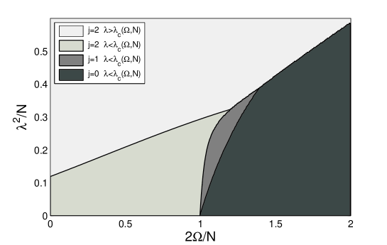
Figure 1: The total momentum angular in the ground-state $j$ as a function of the coupling constant $\lambda$ and the interaction strength $\Omega$ between atoms for $N=4$.

First, we study a finite number of coupled two-level atoms in a cavity. The maximum value of $j$ is $j_{\max}=N/2$. It is very surprising that $j\neq j_{\max}$ in the ground-state for finite systems, unlike in the pure Dicke model. In Fig. 1(a) and (b), we plot the value of j as a function of $\lambda$ and $\Omega^{\prime}=2\Omega/N$ in the ground-state for $N=4$. In the weak interaction of the two-level atoms with small $\Omega^{\prime}$, $j=j_{max}$, similar to the pure dicke model where the interaction of the two- level atoms is neglected. As $\Omega^{\prime}$ increases, the value of $j$ is reduced. In the intermediate coupling range of atom-cavity $\lambda,$ the value of $j$ is reduced gradually by step $1$, until to zero in the strong atomic interaction. This phenomena disappears in the strong coupling range of atom-cavity $\lambda$, where $j$ is always equal to $j_{max}$. For $\lambda=0$, according to Eq. (4), the value of $j$ jumps to zero when the $2\Omega/N=1$, consistent with the observation in Fig. 1. The above observations hold true for any finite number of atoms.

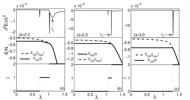
Figure 2: The average ground-state energy $E/N$, its second derivatives $\partial^{2}E/\partial\lambda^{2}$, and the total angular momentum $j$ as a function of $\lambda$ for different atomic interactions $\Omega=2.2$ (a), $\Omega=2.5$ (b), and $\Omega=3.0$ (c) for $N=4$. The dashed lines denote the energy for the total angular momentum $j=j_{max}=N/2$, which is clearly higher the true ground-state energy.

The jump of $j$ in the $\lambda-\Omega$ plane exhibited in Fig. 1 may be related to the first-order QPT in a finite system. It is known that there should be a second-order QPT in this systems without interatomic coupling. Since both the first- and second-order QPTs can be simply characterized by singularities of the ground-state energy, we calculate ground-state energy and its second derivative. These results together with the values of $j$ are collected in Fig. 2 for three typical value of $\Omega$ above the first-order QPT point at $\lambda=0$. For smaller vale of $\Omega=2.2$, two jumps of $j$ indicates two first-order QPTs, as shown in Fig. 2(a). The non-analytic feature of the ground-state energy and sudden drop of its second derivative at the two jump points give the evidence of the first-order QPT. Above the last jump point, the ground-state energy are continuous and its second derivative shows a smooth drop around $\lambda_{c}$, demonstrating a sign of the second-order QPT. $\lambda_{c}(\Omega,N)$ is also presented in Fig. 1, which divides the $j=j_{max}$ regime into two parts. However, as shown in Fig. 2(c), for larger value of $\Omega=3$, there is only one jump of $j$ from $0$ to $j_{max}=N/2$ in the whole coupling regime. Both non-analytic feature of the ground-state energy and sudden drop of its second derivative suggest a first-order QPT at this jump point. No sign of second-order QPT is observed in this case. For the intermediate vale $\Omega=2.5$, two first-order QPTs occur sequentially with the jump of $j$. We think that both the first and the second-order QPT occur in the same point for $\Omega=2.5$ and $3.0$, and finally only the characteristic of the stronger first-order QPT shows up at the last jump.

If we naively set the total angular momentum to be $j_{max}=N/2$ as in the pure Dicke modelchenqh , we can also calculate ”ground-state”, which are also given in Fig. 2 with dashed lines. It is really higher than the true the ground-state energy. The continuous behavior in the whole coupling regime is observed in these dashed curves, demonstrating the above interesting feature in a finite system stems from the variation of the total angular momentum.

Next, we will study the effect of the interatomic interaction on the second-order QPT in the thermodynamical limit. We focuss on the question whether the interatomic interaction alters the universality class of the second-order QPT.

Recently, the fidelity, a concept in quantum information theory, has been extensively used to identify the QPTs in various many-body systems from the perspective of the ground-state wave functionsQuan ; Zanardi ; Cozzini ; You ; Gu ; chens ; zhou ; Kowk . In a mathematical sense, the fidelity is the overlap between two ground states where the transition parameters deviate slightly. However, the fidelity depends on a arbitrary small amount of the transition parameters, which in turn yields an artificial factor. Zanardi et al Cozzini introduced the Riemannian metric tensor and You et al You proposed the fidelity susceptibility (FS) to avoid this problem independently.

To analyze the QPT, we first illustrate the scaling behavior of the average FS. The finite-size scaling ansatz for the average FS take the formKowk

$$\frac{\chi_{F}^{\max}-\chi_{F}}{\chi_{F}}=f[N^{\nu}(\lambda-\lambda_{\max})]$$ (12)

where $\chi_{F}^{\max}$ is the value of average FS at the maximum point $\lambda_{\max}$, $f$ is the scaling function and $\nu$ is the correlation length critical exponent. This function should be universal for large N in the second-order QPTs, which is independent of the order parameter. As shown in Fig. 3 an excellent collapse in the critical regime is achieved with the use of $\nu=2/3$ according to Eq.(12) in the curve for different large size for three values of $\Omega$. It is demonstrated that $\nu$ is a universal constant and does not depended on the parameter $\Omega$, suggesting the interatomic interaction does not change the universality class.

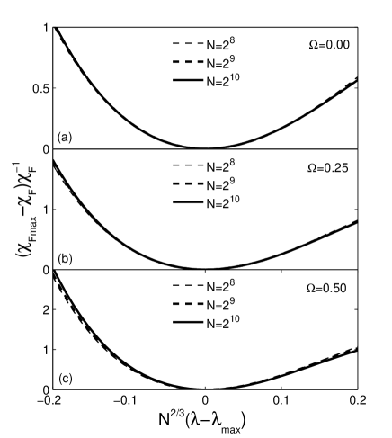
Figure 3: Finite-size scaling of the average FS according to Eq.(12) at the critical point for (a) $\Omega=0$, (b) $\Omega=0.25$, and (c) $\Omega=0.5$.

We then perform the finite size scaling analysis on the order parameter of the QPT, i.e. the expectation value of the photon number per atom in the ground-state $\langle a^{\dagger}a\rangle/N$. In the thermodynamic limit, this quantity changes from zero to finite value smoothly when crossing the critical point. In Fig. 4, we present this quantity as a function of $N$ for different values of $\Omega$ in log-log scale. Derivatives of these curves are plotted in the inset. The exponent of the order parameter is estimated to be ${-0.66\pm 0.01}$ for three values of $\Omega$, provided another piece of the evidence that the interatomic interaction does not change the universality class.

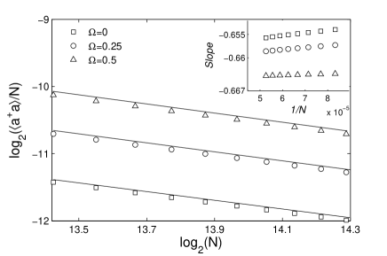
Figure 4: Scaling of the order parameter $\langle a^{\dagger}a\rangle/N$ as a function of $N$ at the critical point for $\Omega=0$, $0.25$, and $0.5$. The inset shows the slope versus $1/N$.

Finally, we calculate the scaled concurrence (entanglement) and perform the corresponding finite size scaling analysis as in Ref. chenqh ; vidal ; reslen . The concurrence quantifies the entanglement between two atoms in the atomic ensemble after tracing out over bosons. In the thermodynamic limit, the scaled concurrence at critical point $C_{\infty}(\lambda_{c})$ can be easily determined with the solution of Eq. (11). For comparison, we can calculate the quantity $C_{\infty}(\lambda_{c})-C_{N}(\lambda_{c})$. In Fig. 5, we present this quantity as a function of $N$ for different values of $\Omega$ in log-log scale. Derivative of these curves is presented in the inset, and the exponent of concurrence is estimated to be ${-0.33\pm 0.005}$ for three values of $\Omega$. This again demonstrates that the universality class is not altered by the interatomic interaction.

Figure 5: Scaling of concurrence as a function of $N$ at the critical point for $\Omega=0$, $0.25$, and $0.5$. The inset show the slope versus $1/N$.

IV Conclusion

In summary, a finite number of dipole-coupled two-level atoms in a single-mode resonant cavity is solved exactly with the use of extended bosonic coherent in the numerically sense. A number ( the maximum value is $N/2$) of first-order QPTs occur in this system with $N$ coupled atoms, different from in the pure Dicke model. The total angular momentum in the ground-state is altered with the coupling constant and the interatomic interactions. The quantum criticality is also studied in terms of the ground-state fidelity, order parameter and concurrence in very large systems up to $2^{10}$ or more. The finite-size scaling analysis for these observables are performed. The corresponding scaling exponents obtained remains unchanged with the interatomic integrations, demonstrating that the university class is not changed. It should be pointed out that all eigenfunctions and eigenvalues obtained in the modified Dicke model on the large scale might also be used to explore the mechanism for the coherent radiation in one-dimensional Josephson arrays coupled to a single-mode cavity at both zero and finite temperatures, which may be our future work.

References

- (1) P. Barbara, A. B. Cawthorne, S. V. Shitov, and C. J. Lobb, Phys. Rev. Lett. 82, 1963 (1999); B. Vasilić, P. Barbara, S.V. Shitov, and C. J. Lobb, Phys. Rev. B 65, 180503 (2002).
- (2) R. H. Dicke, Phys. Rev. 93, 99(1954).
- (3) W. A. Al-Saidi and D. Stroud, Phys. Rev. B 65, 224512 (2002); A. Ballesteros, O. Civitarese, F. J. Herranz, M. Reboiro, Phys. Rev. B 68, 214519 (2003); ; K. Kobayash and D. Stroud, arXiv: 0806.3550v1.
- (4) A. Joshi, R.R. Puri, and S.V. Lawande, Phys. Rev. A 44, 2135 (1991); S.-B. Zheng and G.-C. Guo, Phys. Rev. Lett. 85, 2392 (2000); G. K. Brennen and I. H. Deutsch, and P. S. Jessen, Phys. Rev. A 61, 062309 (2000); A. Blais, R. -S. Huang, A. Wallraff, S. M. Girvin1, and R. J. Schoelkopf, Phys. Rev. A 69, 062320 (2004); P. G. Brooke, K. -P. Marzlin, J. D. Cresser, and B. C. Sanders, Phys. Rev. A 77, 033844 (2008)
- (5) M. Scheibner et al., Nature Phys. 3, 106(2007).
- (6) D. Schneble et al., Science 300, 475 (2003).
- (7) M. J. Hartmann et al., Nature Phys. 2, 849(2006); A. D. Greentree et al., ibid. 2, 856(2006).
- (8) A. Wallraff et al., Nature (London) 431, 162 (2004);R. W. Simmonds et al., Phys. Rev. Lett. 93, 077003(2005).
- (9) Y. Yu et al., Science 296, 889 (2002); I. Chiorescu et al., Science 299, 1869 (2003); I. Chiorescu et al., Nature 431, 159 (2004). J. Johansson et al., Phys. Rev. Lett. 96, 127006 (2006).
- (10) Q. H. Chen, Y. Y. Zhang, T. Liu, and K. L. Wang, Phys. Rev. A 78, 051801(R) (2008); T. Liu, Y. Y. Zhang, Q. H. Chen, and K. L. Wang, Phys. Rev. A 80, 023810(2009).
- (11) B. Peropadre1, P. Forn-Díaz, E. Solano, and J. J. García-Ripoll, Phys. Rev. Lett. 105, 023601 (2010)
- (12) P. Forn-Díaz, J. Lisenfeld, D. Marcos, J. J. García-Ripoll, E. Solano, C. J. P. M. Harmans, and J. E. Mooij, arXiv:1005.1559.
- (13) Q. H. Chen, L. Li, T. Liu, and K. L. Wang, arXiv: 1007.1747.
- (14) C. Emary and T. Brandes, Phys. Rev. E 67, 066203(2003); Phys. Rev. Lett. 90, 044101(2003); N. Lambert, C. Emary, and T. Brandes, Phys. Rev. Lett. 92, 073602(2004)
- (15) N. Lambert, C. Emary, and T. Brandes, Phys. Rev. A. 71, 053804(2005).
- (16) N. Lambert, C. Emary, and T. Brandes, Phys. Rev. Lett. 92, 073602(2004).
- (17) G. Liberti, F. Plastina, and F. Piperno, Phys. Rev. A 74, 022324 (2006).
- (18) J. Vidal and S. Dusuel, Europhys. Lett. 74, 817(2006).
- (19) J. Reslen, L. Quiroga, and N. F. Johnson, Europhys. Lett. 69, 8(2005).
- (20) F. Plastina, G. Liberti, and A. Carollo, Europhys. Lett. 76, 182(2006).
- (21) J. Lipkin, N. Meshkov, and A. J. Glick, Nucl. Phys. 62, 188 (1965).
- (22) H. T. Quan, Z. Song, X. F. Liu, P. Zanardi, and C. P. Sun, Phys. Rev. Lett. 96, 140604 (2006).
- (23) P. Zanardi, and N. Paunković, Phys. Rev. E. 74, 0331123 (2006).
- (24) P. Zanardi, P. Giorda, and M. Cozzini, Phys. Rev. Lett. 99, 100603(2007).
- (25) W. L. You, Y. W. Li, and S. J. Gu, Phys. Rev. E. 76, 022101 (2007).
- (26) S. J. Gu, H. M. Kwok, W. Q. Ning, and H. Q. Lin, Phys. Rev. B. 77, 245109(2008).
- (27) S. Chen, L. Wang, Y. J. Hao, and Y. P. Wang, Phys. Rev. A 77 (2008) 032111.
- (28) H. Q. Zhou, R. Orus, G. Vidal, Phys. Rev. Lett. 100, 080601 (2008); K. W. Sun, Y. Y. Zhang, and Q. H. Chen, Phys. Rev. B. 79, 104429 (2009).
- (29) H. M. Kwok, W. Q. Ning, S. J. Gu, and H. Q. Lin, Phys. Rev. E. 78, 032103 (2008).