Robust Adaptive Beamforming Based on Steering Vector Estimation via Semidefinite Programming Relaxation

Abstract

We develop a new approach to robust adaptive beamforming in the presence of signal steering vector errors. Since the signal steering vector is known imprecisely, its presumed (prior) value is used to find a more accurate estimate of the actual steering vector, which then is used for obtaining the optimal beamforming weight vector. The objective for finding such an estimate of the actual signal steering vector is the maximization of the beamformer output power, while the constraints are the normalization condition and the requirement that the estimate of the steering vector does not converge to an interference steering vector. Our objective and constraints are free of any design parameters of non-unique choice. The resulting optimization problem is a non-convex quadratically constrained quadratic program, which is NP hard in general. However, for our problem we show that an efficient solution can be found using the semi-definite relaxation technique. Moreover, the strong duality holds for the proposed problem and can also be used for finding the optimal solution efficiently and at low complexity. In some special cases, the solution can be even found in closed-form. Our simulation results demonstrate the superiority of the proposed method over other previously developed robust adaptive beamforming methods for several frequently encountered types of signal steering vector errors.

I Introduction

Robust adaptive beamforming design has been an intensive research topic over several decades due to, on one hand, its ubiquitous applicability in wireless communications, radar, sonar, microphone array speech processing, radio astronomy, medical imaging, and so on; and on the other hand, because of the challenges related to the practical applications manifesting themselves in the robustness requirements for adaptive beamformers. The main causes of performance degradation in adaptive beamforming are small sample size and imprecise knowledge of the desired signal steering vector in the situation when the desired signal components are present in the training data. The traditional design approaches to adaptive beamforming [1]-[4] do not provide sufficient robustness and are not applicable in such situations. Thus, various robust adaptive beamforming techniques gained a significant popularity due to their practical importance [5]. The most popular conventional robust adaptive beamforming approaches are the diagonal loading technique [6], [7] and the eigenspace-based beamforming technique [8], [9]. However, it is not clear in the former approach how to obtain the optimal value of the diagonal loading factor, whereas the eigenspace-based beamforming is known to suffer from the so-called subspace swap phenomenon at low signal-to-noise ratios (SNRs) [10] and requires exact knowledge of the signal-plus-interference subspace dimension.

In the last decade, several approaches to robust adaptive beamforming based on a rigorous modeling of the steering vector mismatches have been developed. For the case when the mismatch of the signal steering vector is modeled as deterministic unknown norm bounded vector, the so-called worst-case-based adaptive beamforming design has been proposed in [11], [12]. The relationship of the worst-case-based design to the diagonal loading principle with adaptive diagonal loading factor has been explored in [11], [13] as well as the generalization to the ellipsoidal steering vector uncertainty set has been developed in[14]. The uncertainty of second order statistics of the desired signal have been also considered in [15]. If the signal steering vector mismatch is modeled as random unknown with known Gaussian or unknown distribution, the corresponding optimization problem belongs to the class of stochastic programming problems, and the corresponding probabilistically-constrained robust adaptive beamformer has been developed in [16], [17]. The relationship between the worst-case-based and the probabilistically-constrained robust adaptive beamformers has also been shown in [17], [18]. However, some design parameters such as the norm of the signal steering vector mismatch in the worst-case-based design or the acceptable beamforming outage probability in the probabilistically-constrained design are assumed to be known in the aforementioned techniques.

Another approach to robust adaptive beamforming which is based on estimating actual signal steering vector based on the knowledge of presumed steering vector has been proposed in [19], [20]. The main idea of this approach is to estimate the signal steering vector so that the maximum of the beamformer output power is achieved, while the convergence of the steering vector estimate to an interference steering vector is avoided. The latter convergence can be avoided by imposing different constraints. The projection constraint to the space to which the desired signal belongs is used in [20] and the solution based on sequential quadratic programming (SQP) is developed. The advantage of the method of [20] is that no design parameters of non-unique choice are required. However, the disadvantage is that the complexity of SQP is rather high, which makes the method less attractive for practical use. It is interesting that the robust adaptive beamforming formulation based on desired signal steering vector estimation has been also considered in [21], but the typical for the worst-case-based methods [11]-[14] norm bound constraint on the steering vector mismatch has been used there in order to guarantee that the estimate of the desired signal steering vector does not converge to an interference steering vector. As a result, the method of [21] is one of the various implementations of the adaptive diagonal loading based techniques, and it is not free of design parameters.

In this paper, we develop a new robust adaptive beamforming method which is free of any design parameters of non-unique choice. This method is based on the signal steering vector estimation via beamformer output power maximization under the constraint on the norm of the steering vector estimate and the requirement that the estimate of the steering vector does not converge to an interference steering vector. To satisfy the latter requirement, we develop a new constraint which is a convex quadratic constraint. Then the corresponding optimization problem is a non-convex (due to the steering vector normalization condition) homogeneous quadratically constrained quadratic programming (QCQP) problem. In general, QCQP problems may not have a strong duality property, which leads to the situation when the solution of the corresponding semidefinite programming (SDP) relaxation-based problem is of rank higher than one and randomization procedures have to be used to find an approximate rank-one solution [23]-[26]. The probability that the so-obtained rank-one solution coincides with the exact solution is less than one [27]. However, in the case of our signal steering vector estimation problem, we show that a rank-one solution can be found efficiently using the SDP relaxation technique. Moreover, the strong duality holds for the proposed problem, which means that a rank-one solution can also be found based on the solution of the convex dual problem. Some special cases and interesting relationships are also considered. Our simulation results demonstrate the superiority of the proposed method over other previously developed robust adaptive beamforming techniques.

This paper is organized as follows. Data model, beamforming formulation, and necessary background are given in Section II. In Section III, we formulate the problem of interest. A complete analysis of the problem and its rank-one solution is given in Section IV. Section V overviews some special cases and draws interesting relations to the existing methods. Simulation results comparing the performance of the proposed method to the existing methods are shown in Section VI. Finally, Section VII presents our conclusions.

II System Model and Background

Consider a linear antenna array with $M$ omni-directional antenna elements. The narrowband signal received by the antenna array at the time instant $k$ can be written as

$$\mathbf{x}(k)=\mathbf{s}(k)+\mathbf{i}(k)+\mathbf{n}(k)$$ (1)

where $\mathbf{s}(k)$, $\mathbf{i}(k)$, and $\mathbf{n}(k)$ denote the $M\times 1$ vectors of the desired signal, interference, and noise, respectively. The desired signal, interference, and noise components of the received signal (1) are assumed to be statistically independent to each other. The desired signal can be written as $\mathbf{s}(k)=s(k)\mathbf{a}$, where $s(k)$ is the desired signal waveform and $\mathbf{a}$ is the steering vector associated with the desired signal.

The beamformer output at the time instant $k$ can be written as

$$y(k)=\mathbf{w}^{H}\mathbf{x}(k)$$ (2)

where $\mathbf{w}$ is the $M\times 1$ complex weight (beamforming) vector of the antenna array and $(\cdot)^{H}$ stands for the Hermitian transpose.

Assuming that the steering vector $\mathbf{a}$ is known precisely, the optimal weight vector can be obtained by maximizing the beamformer output signal-to-noise-plus-interference ratio (SINR) [1]

$${SINR}=\frac{\sigma_{\rm s}^{2}|\mathbf{w}^{H}\mathbf{a}|^{2}}{\mathbf{w}^{H}\mathbf{R}_{i+n}\mathbf{w}}$$ (3)

where $\sigma_{\rm s}^{2}$ is the desired signal power, $\mathbf{R}_{i+n}\triangleq E\{(\mathbf{i}(k)+\mathbf{n}(k))(\mathbf{i}(k)+\mathbf{n}(k))^{H}\}$ is the $M\times M$ interference-plus-noise covariance matrix, and $E\{\cdot\}$ stands for the statistical expectation. Since $\mathbf{R}_{i+n}$ is unknown in practice, it is substituted in (3) by the data sample covariance matrix

$$\hat{\mathbf{R}}=\frac{1}{K}\sum_{i=1}^{K}\mathbf{x}(i)\mathbf{x}^{H}(i)$$ (4)

where $K$ is the number of training data samples which also include the desired signal component. The sample version of the problem of maximizing (3) is known as the minimum variance (MV) sample matrix inversion (SMI) beamforming and it is based on its conversion to the mathematically equivalent problem of minimizing the denominator of (3) under fixed numerator, that is,

$$\min_{\mathbf{w}}\mathbf{w}^{H}\hat{\mathbf{R}}\mathbf{w}\quad{\rm subject\ to}\quad\mathbf{w}^{H}\mathbf{a}=1.$$ (5)

The problem (5) is convex and its solution can be easily found as ${\mathbf{w}}_{\rm MV-SMI}=\alpha\hat{\mathbf{R}}^{-1}\mathbf{a}$ where $\alpha=1/\mathbf{a}^{H}\hat{\mathbf{R}}^{-1}\mathbf{a}$ [1].

In practice, the steering vector $\mathbf{a}$ is not known precisely and only its inaccurate estimate $\mathbf{p}$, called hereafter as presumed steering vector, is available. Several rigorous approaches, which address the problem of imprecise knowledge of the desired signal steering vector have been developed in the last decade. First of them assumes that the actual steering vector $\mathbf{a}$ can be explicitly modeled as a sum of the presumed steering vector and a deterministic mismatch vector $\boldsymbol{\delta}$, i.e., $\mathbf{a}=\mathbf{p}+\boldsymbol{\delta}$ [11], [12]. Here $\boldsymbol{\delta}$ is unknown but it is known that $\|\boldsymbol{\delta}\|\leq\varepsilon$ for some bound value $\varepsilon$, where $\|\cdot\|$ is the Euclidian norm of a vector. This approach has been also generalized for ellipsoidal uncertainty case in addition to the aforementioned spherical uncertainty [14]. Assuming spherical uncertainty set for $\boldsymbol{\delta}$, i.e., $\cal{A}(\varepsilon)\triangleq\{\mathbf{a}=\mathbf{p}+{\boldsymbol{\delta}}\,|\,\|\boldsymbol{\delta}\|\leq\varepsilon\}$, the worst-case-based robust adaptive beamforming aims at solving the following optimization problem

$$\min_{\mathbf{w}}\mathbf{w}^{H}\hat{\mathbf{R}}\mathbf{w}\quad{\rm subject\ to}\quad\max_{\mathbf{a}\in\cal{A}(\varepsilon)}|\mathbf{w}^{H}\mathbf{a}|\geq 1.$$ (6)

In turn, the problem (6) is equivalent to the following convex optimization problem [11]

$$\min_{\mathbf{w}}\mathbf{w}^{H}\hat{\mathbf{R}}\mathbf{w}\quad{\rm subject\ to}\quad\varepsilon\|\mathbf{w}\|\leq\mathbf{w}^{H}\mathbf{p}-1$$ (7)

which can be efficiently solved using second-order cone programming (SOCP) [11], [28] or numerical Lagrange multiplier techniques [14], [29].

Another approach to robust adaptive beamforming is based on the assumption that the vector $\boldsymbol{\delta}$ is random. Then the problem (6) changes to

$$\min_{\mathbf{w}}\mathbf{w}^{H}\hat{\mathbf{R}}\mathbf{w}\quad{\rm subject\ to}\quad{\rm Pr}\{|\mathbf{w}^{H}\mathbf{a}|\geq 1\}\geq p_{0}$$ (8)

where ${\rm Pr}\{\cdot\}$ denotes probability and $p_{0}$ is preselected probability value. In the case of Gaussian distributed $\boldsymbol{\delta}$ and the case when the distribution of $\boldsymbol{\delta}$ is unknown and assumed to be the worst possible, it has been shown that the problem (8) can be approximated by the following problem [17], [18],

$$\min_{\mathbf{w}}\mathbf{w}^{H}\hat{\mathbf{R}}\mathbf{w}\quad{\rm subject\ to}\quad\tilde{\varepsilon}\|\mathbf{Q}_{\delta}^{1/2}\mathbf{w}\|\leq\mathbf{w}^{H}\mathbf{p}-1$$ (9)

where $\mathbf{Q}_{\delta}$ is the covariance matrix of random mismatch vector $\boldsymbol{\delta}$, and $\tilde{\varepsilon}=\sqrt{-\ln(1-p_{0})}$ if $\boldsymbol{\delta}$ is Gaussian distributed or $\tilde{\varepsilon}=1/\sqrt{1-p_{0}}$ if the distribution of $\boldsymbol{\delta}$ is unknown. Both problems (7) and (9) have similar SOCP structure and can be solved efficiently.

The third approach to robust adaptive beamforming aims at estimating the steering vector $\mathbf{a}$ based on the prior given by the presumed steering vector $\mathbf{p}$ [19], [20]. The estimate of the steering vector $\mathbf{a}$ is found so that the beamformer output power is maximized while the convergence of the estimate of $\mathbf{a}$ to any interference steering vector is prohibited. Indeed, the solution of (5) can be written as a function of unknown $\boldsymbol{\delta}$, that is, $\mathbf{w}({\boldsymbol{\delta}})=\alpha\hat{\mathbf{R}}^{-1}(\mathbf{p}+\boldsymbol{\delta})$. Using the latter expression, the beamformer output power can be also written as a function of $\boldsymbol{\delta}$ as

$$P({\boldsymbol{\delta}})=\frac{1}{(\mathbf{p}+\boldsymbol{\delta})^{H}\hat{\mathbf{R}}^{-1}(\mathbf{p}+\boldsymbol{\delta})}.$$ (10)

Thus, such estimate of $\boldsymbol{\delta}$ or, equivalently, such estimate of $\mathbf{a}$ that maximizes (10) will be the best estimate of the actual steering vector $\mathbf{a}$ under the constraints that the norm of $\hat{\mathbf{a}}$ equals $\sqrt{M}$ and $\hat{\mathbf{a}}$ does not converge to any of the interference steering vectors. The latter can be guaranteed by requiring that

$$\mathbf{P}^{\bot}(\mathbf{p}+\hat{\boldsymbol{\delta}})=\mathbf{P}^{\bot}\hat{\mathbf{a}}=0$$ (11)

where $\mathbf{P}^{\bot}=\mathbf{I}-\mathbf{U}\mathbf{U}^{H}$, $\mathbf{U}=[\mathbf{u}_{1},\mathbf{u}_{2},\ldots,\mathbf{u}_{L}]$, $\mathbf{u}_{l}$, ${l=1},\ldots,L$ are the $L$ dominant eigenvectors of the matrix $\mathbf{C}=\int_{\Theta}\mathbf{d}(\theta)\mathbf{d}^{H}(\theta)\,d\theta$, $\mathbf{d}(\theta)$ is the steering vector associated with direction $\mathbf{\theta}$ and having the structure defined by the antenna geometry, $\Theta$ is the angular sector in which the desired signal is located, $\hat{\boldsymbol{\delta}}$ and $\hat{\boldsymbol{a}}$ stand for the estimate of the steering vector mismatch and for the estimate of the actual steering vector, respectively and $\mathbf{I}$ is the identity matrix. The resulting optimization problem is non-convex, but has been solved in [20] using SQP technique. A similar approach based on steering vector estimation has been also recently taken in [30] for the case when $\mathbf{a}$ is partially known, for example, when array is partially calibrated, that significantly simplifies the problem. The following interesting relationship is also worth mentioning. If the constraint (11) is replaced by the constraint $\|\boldsymbol{\delta}\|\leq\varepsilon$ used in the worst-case-based beamformers, the convergence to an interference steering vector will also be avoided, but the problem becomes equivalent to the worst-case-based robust adaptive beamforming (see [21]).

Finally, it is worth mentioning that the eigenspace-based beamformer [8], [9] is also based on correcting/estimating the desired signal steering vector. Taking the presumed steering vector $\mathbf{p}$ as a prior, the eigenspace-based beamformer finds and uses the projection of $\mathbf{p}$ onto the sample signal-plus-interference subspace as a corrected estimate of the steering vector. The eigendecomposition of (4) yields

$$\hat{\mathbf{R}}=\mathbf{E}\boldsymbol{\Lambda}\mathbf{E}^{H}+\mathbf{G}\boldsymbol{\Gamma}\mathbf{G}^{H}$$ (12)

where the $M\times J+1$ matrix $\mathbf{E}$ and $M\times M-J-1$ matrix $\mathbf{G}$ contain the signal-plus-interference subspace eigenvectors of $\hat{\mathbf{R}}$ and the noise subspace eigenvectors, respectively, while the $J+1\times J+1$ matrix $\boldsymbol{\Lambda}$ and $M-J-1\times M-J-1$ matrix $\boldsymbol{\Gamma}$ contain the eigenvalues corresponding to $\mathbf{E}$ and $\mathbf{G}$, respectively. Here, $J$ is the number of interfering signals. Then the eigenspace-based beamformer is given by

$$\mathbf{w}_{\rm eig}=\hat{\mathbf{R}}^{-1}\hat{\mathbf{a}}=\hat{\mathbf{R}}^{-1}\mathbf{E}\mathbf{E}^{H}\mathbf{p}=\mathbf{E}\boldsymbol{\Lambda}^{-1}\mathbf{E}^{H}\mathbf{p}$$ (13)

where $\hat{\mathbf{a}}=\mathbf{E}\mathbf{E}^{H}\mathbf{p}$ is the projection of the presumed steering vector $\mathbf{p}$ onto the sample signal-plus-interference subspace and $\mathbf{E}\mathbf{E}^{H}$ is the corresponding projection matrix. As compared to the beamformer of [20] based on the estimation of steering vector, the eigenspace-based beamformer may suffer from a high probability of subspace swaps as well as incorrect estimation of the signal-plus-interference subspace dimension.

III New beamforming Problem Formulation

The problem of maximizing the output power (10) is equivalent to the problem of minimizing the denominator of (10). The obvious constraint that must be imposed on the estimate $\hat{\mathbf{a}}$, is that the norm of $\hat{\mathbf{a}}$ must be equal to $\sqrt{M}$, i.e., $\|\hat{\mathbf{a}}\|=\sqrt{M}$. This normalization condition, however, does not protect the estimate $\hat{\mathbf{a}}$ from possible convergence to an interference steering vector. In order to avoid such convergence, we assume that the desired source is located in the angular sector $\Theta=[\theta_{\min},\,\theta_{\max}]$ which can be obtained, for example, using low resolution direction finding methods. The angular sector $\Theta$ is assumed to be distinguishable from general locations of all interfering signals. In turns, the sector $\tilde{\Theta}$ denotes the complement of the sector $\Theta$, i.e., combines all the directions which lie outside of $\Theta$. Let us define the $M\times M$ matrix $\tilde{\mathbf{C}}$ as $\tilde{\mathbf{C}}=\int_{\tilde{\Theta}}{\mathbf{d}(\theta)\mathbf{d}^{H}(\theta)\,d\theta}$. Then constraint

$$\hat{\mathbf{a}}^{H}\tilde{\mathbf{C}}\hat{\mathbf{a}}\leq\Delta_{0}$$ (14)

for a uniquely selected value $\Delta_{0}$ (see Example 1 below), will force the estimate $\hat{\mathbf{a}}$ not to converge to any interference steering vector with the directions within the angular sector $\tilde{\Theta}$. To illustrate how the constraint (14) works, let us consider the following example.

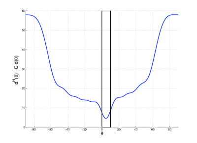
Figure 1: The term $\mathbf{d}^{H}(\theta)\tilde{\mathbf{C}}\mathbf{d}(\theta)$ in the constraint (14) versus different angles.

Example 1: Consider uniform linear array (ULA) of $10$ omni-directional antenna elements spaced half wavelength apart from each other. Let the range of the desired signal angular locations be $\Theta=[0^{\circ},\,10^{\circ}]$. Fig. 1 depicts the values of the quadratic term $\mathbf{d}^{H}(\theta)\tilde{\mathbf{C}}\mathbf{d}(\theta)$ for different angles. The rectangular bar in the figure marks the directions within the angular sector $\Theta$. It can be observed from this figure that the term $\mathbf{d}^{H}(\theta)\tilde{\mathbf{C}}\mathbf{d}(\theta)$ takes the smallest values within the angular sector $\Theta$, where the desired signal is located, and increases outside of this sector. Therefore, if $\Delta_{0}$ is selected to be equal to the maximum value of the term $\mathbf{d}^{H}(\theta)\tilde{\mathbf{C}}\mathbf{d}(\theta)$ within the angular sector of the desired signal $\Theta$, the constraint (14) will guarantee that the estimate of the desired signal steering vector will not converge to any interference steering vectors. Note also that the constraint (14) is an alternative to the constraint (11) used in [20]. However, the constraint (11) may result in the noise power magnification at low SNRs (see [20]), while the constraint (14) helps to alleviate the effect of the noise power magnifying at low SNRs by not collecting the noise power from the continuum of the out-of-sector directions $\tilde{\Theta}$.

Taking into account the normalization constraint and the constraint (14), the problem of estimating the desired signal steering vector based on the knowledge of the prior $\mathbf{p}$ can be formulated as the following optimization problem

$$\min_{\hat{\mathbf{a}}} \hat{\mathbf{a}}^{H}\hat{\mathbf{R}}^{-1}\hat{\mathbf{a}}$$ (15)

$${\rm subject\ to} \left\|\hat{\mathbf{a}}\right\|=\sqrt{M}$$ (17)

$$\hat{\mathbf{a}}^{H}\tilde{\mathbf{C}}\hat{\mathbf{a}}\leq\Delta_{0}.$$

where the prior $\mathbf{p}$ is used only for selecting the sector $\Theta$. Due to the equality constraint (17), which is a non-convex one, the QCQP problem of type (15)–(17) is non-convex and an NP-hard in general. However, as we show in the following section, an exact and simple solution specifically for the problem (15)–(17) can be found using the SDP relaxation technique and the strong duality theory.

IV Steering Vector Estimation via Semi-Definite Programming Relaxation

QCQP problems of type (15)–(17) can be solved using SDP relaxation technique. The first step is to make sure that the problem (15)–(17) is feasible. Fortunately, it can be easily verified that (15)–(17) is feasible if and only if $\Delta_{0}/M$ is greater than or equal to the smallest eigenvalue of the matrix $\tilde{\mathbf{C}}$. Indeed, if the smallest eigenvalue of $\tilde{\mathbf{C}}$ is larger than $\Delta_{0}/M$, then the constraint (17) can not be satisfied for any estimate $\hat{\mathbf{a}}$. However, $\Delta_{0}$ selected as suggested in Example 1 will satisfy the feasibility condition that will guarantee the feasibility of the problem (15)–(17).

IV-A Semi-Definite Programming Relaxation

If the problem (15)–(17) is feasible, the equalities $\hat{\mathbf{a}}^{H}\hat{\mathbf{R}}^{-1}\hat{\mathbf{a}}=Tr(\hat{\mathbf{R}}^{-1}\hat{\mathbf{a}}\hat{\mathbf{a}}^{H})$ and $\hat{\mathbf{a}}^{H}\tilde{\mathbf{C}}\hat{\mathbf{a}}=Tr(\tilde{\mathbf{C}}\hat{\mathbf{a}}\hat{\mathbf{a}}^{H})$, where $Tr(\cdot)$ denotes the trace of a matrix, can be used to rewrite it as the following optimization problem

$$\min_{\hat{\mathbf{a}}} Tr(\hat{\mathbf{R}}^{-1}\hat{\mathbf{a}}\hat{\mathbf{a}}^{H})$$ (18)

$${\rm subject\ to} Tr(\hat{\mathbf{a}}\hat{\mathbf{a}}^{H})=M$$ (20)

$$Tr(\tilde{\mathbf{C}}\hat{\mathbf{a}}\hat{\mathbf{a}}^{H})\leq\Delta_{0}.$$

Introducing the new variable $\mathbf{A}=\hat{\mathbf{a}}\hat{\mathbf{a}}^{H}$, the problem (18)–(20) can be casted as

$$\min_{\mathbf{A}} Tr(\hat{\mathbf{R}}^{-1}\mathbf{A})$$ (21)

$${\rm subject\ to} Tr(\mathbf{A})=M$$ (24)

$$Tr(\tilde{\mathbf{C}}\mathbf{A})\leq\Delta_{0}$$

$$rank(\mathbf{A})=1$$

where $rank(\cdot)$ stands for the rank of a matrix and it is guaranteed by the combination of the constraints (24) and (24) that $\mathbf{A}$ is a positive semi-definite matrix, i.e., $\mathbf{A}\succeq\mathbf{0}$.

The only non-convex constraint in the problem (21)–(24) is the rank-one constraint (24) while all other constraints and the objective are convex. Using the SDP relaxation technique, the relaxed problem can be obtained by dropping the non-convex rank-one constraint (24) and replacing it by the semi-definiteness constraint $\mathbf{A}\succeq\mathbf{0}$, which otherwise is not guaranteed if (24) is not present. Thus, the problem (21)–(24) is replaced by the following relaxed convex problem

$$\min_{\mathbf{A}} Tr(\hat{\mathbf{R}}^{-1}\mathbf{A})$$ (25)

$${\rm subject\ to} Tr(\mathbf{A})=M$$ (28)

$$Tr(\tilde{\mathbf{C}}\mathbf{A})\leq\Delta_{0}$$

$$\mathbf{A}\succeq\mathbf{0}.$$

There are two features related to the use of SDR that have to be addressed. First, it is possible, in general, that the original problem is infeasible, however the relaxed one is feasible. Second, the optimal solution of the relaxed problem is, in general, an approximation of the optimal solution of the original problem. Thus, it is desirable in general to estimate the approximation bounds for the approximate solution and the probability that both approximate and exact optimal solutions coincide [27]. In the following we will address these issues.

IV-B Feasibility and Rank of the Optimal Solution

The result that connects the feasibility of the relaxed problem (25)–(28) to the feasibility of the original problem (15)-(17) is given in terms of the following theorem.

Theorem 1: The problem (25)–(28) is feasible if and only if the problem (15)–(17) is feasible.

Proof: See Appendix.

If the relaxed problem (25)–(28) has a rank-one solution, then the principle eigenvector of the solution of (25)–(28) will be the exact solution to the original problem (15)–(17). Otherwise, randomization procedures [25], [26] have to be used, which can find the exact optimal solution of the original problem only with a certain probability [27]. However, under the condition that the original optimization problem (15)–(17) or, equivalently, the relaxed problem (25)–(28) is feasible, the solution of the original problem can be extracted from the solution of the relaxed problem by means of the following constructive theorem.

Theorem 2: Let $\mathbf{A}^{*}$ be the rank $r$ optimal minimizer of the relaxed problem (25)–(28), i.e., $\mathbf{A}^{*}=\mathbf{Y}\mathbf{Y}^{H}$ (where $\mathbf{Y}$ is an ${N\times r}$ matrix). If $r=1$, the optimal solution of the original problem simply equals $\mathbf{Y}$. Otherwise, it equals $\mathbf{Y}\mathbf{v}$, where $\mathbf{v}$ is an $r\times 1$ vector such that $\|\mathbf{Y}\mathbf{v}\|=\sqrt{M}$ and $\mathbf{v}^{H}\mathbf{Y}^{H}\tilde{\mathbf{C}}\mathbf{Y}\mathbf{v}=Tr(\mathbf{Y}^{H}\tilde{\mathbf{C}}\mathbf{Y})$. Then one possible solution for the vector $\mathbf{v}$ is proportional to the sum of the eigenvectors of the following $r\times r$ matrix

$$\mathbf{D}=\frac{1}{M}\mathbf{Y}^{H}\mathbf{Y}-\frac{\mathbf{Y}^{H}\tilde{\mathbf{C}}\mathbf{Y}}{Tr(\mathbf{Y}^{H}\tilde{\mathbf{C}}\mathbf{Y})}.$$ (29)

Proof: See Appendix.

Finally, we can prove the following result on the uniqueness of the rank-one solution of the relaxed problem (25)–(28).

Theorem 3: Under the condition that the solution of the original optimization problem (15)–(17) is unique regardless of a phase shift, where the latter means that if $\hat{\mathbf{a}}$ and $\hat{\mathbf{a}}^{\prime}$ are both optimal solutions, then there exists such phase shift $\phi$ that $\hat{\mathbf{a}}=\hat{\mathbf{a}}^{\prime}e^{j\phi}$, the solution of the relaxed problem (25)–(28) always has rank one.

Proof: See Appendix.

Note that the phase shift plays no role in the desired signal steering vector estimation problem since the output power (10) as well as the output SINR do not change if $\hat{\mathbf{a}}$ undergo any phase rotation. Thus, the uniqueness condition regardless a phase shift in Theorem 3 is proper . Under this condition, the solution of the relaxed problem (25)–(28) is rank-one and the solution of the original problem (15)–(17) can be found as a dominant eigenvector of the optimal solution of the relaxed problem (25)–(28). However, even such uniqueness condition regardless a phase shift is not necessarily satisfied for the problem (15)–(17) (see Example 2 below), and then we resort to the constructive Theorem 2, which shows how to find the rank-one solution of (15)–(17) algebraically without any use of randomization procedures.

Example 2: As an example of the situation when (15)–(17) does not have a unique solution, let us consider a ULA with 10 omni-directional antenna elements. The presumed direction of arrival of the desired user is assumed to be $\theta_{p}=3^{\circ}$ with no interfering sources and the range of the desired signal angular locations is equal to $\Theta=[\theta_{p}-12^{\circ},\theta_{p}+12^{\circ}]$. The actual steering vector of the desired user is perturbed due to the incoherent local scattering effect and it can be expressed as $\mathbf{a}=\mathbf{p}+\mathbf{b}$, where $\mathbf{p}=\mathbf{d}(3^{\circ})$ is the steering vector of the direct path and $\mathbf{b}$ is the steering vector of the coherently scattered path. Let us consider the case when $\mathbf{b}$ is orthogonal to $\mathbf{p}$. This later condition can be satisfied if $\mathbf{b}$ is selected as $\mathbf{d}(-8.5^{\circ})$. In this case, both of the vectors $\mathbf{p}$ and $\mathbf{b}$ are the eigenvectors of the matrix $\mathbf{R}^{-1}$ which correspond to the smallest eigenvalue. Since, these vectors satisfy the constraints (17)–(17) and correspond to the minimum eigenvalue, both of them are optimal solutions of the optimization problem (15)-(17), thus, the solution of the problem (15)–(17) is not unique.

IV-C Solution Based on Strong Duality

The solution of (15)–(17) can also be found using the strong duality theory. It follows from Theorem 2 that the optimal value of the relaxed problem (25)–(28) is the same as the optimal value of the the original problem (15)–(17). It is because in addition to the fact that $\mathbf{Y}\mathbf{v}$ is the optimal solution of the original problem (15)–(17) (see Theorem 2), $\mathbf{Y}\mathbf{v}(\mathbf{Y}\mathbf{v})^{H}$ is also the optimal solution of the relaxed problem (25)–(28) (see the proof of Theorem 2). Furthermore, the dual problem of the the relaxed problem (25)–(28) is the same as the dual problem of the original problem (15)–(17). Indeed, by maximizing the dual function of the problem (25)–(28), which is the same as the dual function of (15)–(17), the dual problem for both the relaxed and original problems can be written as

$$\max_{\gamma_{1},\gamma_{2}} \gamma_{1}M-\gamma_{2}\Delta_{0}$$ (30)

$${\rm subject\ to} \hat{\mathbf{R}}^{-1}-\gamma_{1}\mathbf{I}+\gamma_{2}\tilde{\mathbf{C}}\succeq\mathbf{0}$$ (31)

where $\gamma_{1}$ and $\gamma_{2}\geq 0$ are the Lagrange multipliers associated with constraints (17) and (17) of the original problem or the constraints (28) and (28) of the relaxed problem, respectively. Since the relaxed problem (25)–(28) is convex, the strong duality between (25)–(28) and (30)–(31) holds, i.e., the optimal value of (25)–(28) is the same as the optimal value of (30)–(31). It implies that the optimal value of the dual problem (30)–(31) is also the same as the optimal value of the original problem (15)–(17). Thus, the strong duality between the dual problem (30)–(31) and the original problem (15)–(17) also holds. It is worth mentioning that the strong duality of a non-convex quadratic optimization problem with two positive semi-definite quadratic constraints has been also studied in the recent work [31]. Particularly, it has been shown that if a non-convex quadratic optimization problem with two quadratic constraints is strictly feasible, then strong duality holds. This result agrees with our above conclusion that the strong duality between (30)–(31) and (15)–(17) holds. Indeed, it can be easily shown that if $\Delta_{0}/M$ is greater than the smallest eigenvalue of the matrix $\tilde{\mathbf{C}}$, then the problem (15)–(17) is strictly feasible, and thus the result of [31], [32] applies and the strong duality between (30)–(31) and (15)–(17) holds. Moreover, if $\Delta_{0}/M$ is equal to the smallest eigenvalue of the matrix $\tilde{\mathbf{C}}$, the problem (15)–(17) has limited number of feasible points and it can be solved easily by checking all these points. Thus, it is simply assumed in the sequel that $\Delta_{0}/M$ is greater than the smallest eigenvalue of $\tilde{\mathbf{C}}$.

The dual problem (30)–(31) belongs to the class of SDP problems and, thus, can be solved efficiently using, for example, interior-point methods. Moreover, it contains only two optimization variables. Let the optimal solution of the the dual problem (30)–(31) be $\gamma_{1}^{*}$ and $\gamma_{2}^{*}$. It is easy to see that $\gamma_{1}^{*}$ is always strictly positive and the matrix $\hat{\mathbf{R}}^{-1}-\gamma_{1}^{*}\mathbf{I}+\gamma_{2}^{*}\tilde{\mathbf{C}}$ is rank deficient. Indeed, in order to maximize the objective function (30) for a fixed $\gamma_{2}\geq 0$, $\gamma_{1}$ should be equal to the smallest eigenvalue of the matrix $\hat{\mathbf{R}}^{-1}+\gamma_{2}\tilde{\mathbf{C}}$ which makes the matrix $\hat{\mathbf{R}}^{-1}-\gamma_{1}\mathbf{I}+\gamma_{2}\tilde{\mathbf{C}}$ rank deficient. Furthermore, since for every nonnegative $\gamma_{2}$, $\hat{\mathbf{R}}^{-1}+\gamma_{2}\tilde{\mathbf{C}}$ is a positive definite matrix, we obtain that $\gamma_{1}^{*}$ is positive and $\hat{\mathbf{R}}^{-1}-\gamma_{1}\mathbf{I}+\gamma_{2}\tilde{\mathbf{C}}$ is rank deficient. Since the strong duality between (15)–(17) and (30)–(31) holds, the necessary and sufficient optimality conditions can be written as

$$(\hat{\mathbf{R}}^{-1}-\gamma_{1}^{*}\mathbf{I}+\gamma_{2}^{*}\tilde{\mathbf{C}})\hat{\mathbf{a}}=\mathbf{0}_{M}$$ (32)

$$\hat{\mathbf{a}}^{H}\hat{\mathbf{a}}=M$$ (33)

$$\gamma_{2}^{*}(\hat{\mathbf{a}}^{H}\tilde{\mathbf{C}}\hat{\mathbf{a}}-\Delta_{0})=0$$ (34)

$$\hat{\mathbf{a}}^{H}\tilde{\mathbf{C}}\hat{\mathbf{a}}\leq\Delta_{0}.$$ (35)

where $\mathbf{0}_{M}$ is the vector of zeros of length $M$. Moreover, using the fact that $\gamma_{1}^{*}$ is strictly positive and the matrix $\hat{\mathbf{R}}^{-1}-\gamma_{1}^{*}\mathbf{I}+\gamma_{2}^{*}\tilde{\mathbf{C}}$ is rank deficient, the solution of the original problem (15)–(17) can easily be found. There are two possible situations.

• The matrix $\hat{\mathbf{R}}^{-1}-\gamma_{1}^{*}\mathbf{I}+\gamma_{2}^{*}\tilde{\mathbf{C}}$ has only one zero eigenvalue. In this case, the only vector which satisfies (32) is given by

  $$\hat{\mathbf{a}}=\sqrt{M}\boldsymbol{\rho}\left\{\hat{\mathbf{R}}^{-1}-\gamma_{1}^{*}\mathbf{I}+\gamma_{2}^{*}\tilde{\mathbf{C}}\right\}$$ (36)

  where $\boldsymbol{\rho}\{\cdot\}$ denotes the eigenvector of a matrix which corresponds to the smallest eigenvalue. Indeed, (36) satisfies the necessary and sufficient optimality conditions (32)–(35) and, thus, is the optimal solution of (15)–(17).

• The matrix $\hat{\mathbf{R}}^{-1}-\gamma_{1}^{*}\mathbf{I}+\gamma_{2}^{*}\tilde{\mathbf{C}}$ has more than one zero eigenvalue. In this case, consider the matrix $\mathbf{F}$ each column of which is an eigenvector of the matrix $\hat{\mathbf{R}}^{-1}-\gamma_{1}^{*}\mathbf{I}+\gamma_{2}^{*}\tilde{\mathbf{C}}$ corresponding to zero eigenvalue. Thus, the dimension of $\mathbf{F}$ is $M\times q$ where $q$ is the number of zero eigenvalues of the matrix $\hat{\mathbf{R}}^{-1}-\gamma_{1}^{*}\mathbf{I}+\gamma_{2}^{*}\tilde{\mathbf{C}}$. Then vectors $\hat{\mathbf{a}}$ that satisfy the condition (32) can be written as

  $$\hat{\mathbf{a}}=\mathbf{F}\mathbf{q}$$ (37)

  where $\mathbf{q}$ is a ${k\times 1}$ vector. The optimality conditions (32)–(35) can be rewritten then in terms of $\mathbf{q}$ and $\mathbf{F}$ as

  $$\mathbf{q}^{H}\mathbf{q}=M$$ (38)

  $$\gamma_{2}^{*}(\mathbf{q}^{H}\mathbf{F}^{H}\tilde{\mathbf{C}}\mathbf{F}\mathbf{q}-\Delta_{0})=0$$ (39)

  $$\mathbf{q}^{H}\mathbf{F}^{H}\tilde{\mathbf{C}}\mathbf{F}\mathbf{q}\leq\Delta_{0}.$$ (40)

  Let $\mu_{max}$ and $\mu_{min}$ denote the largest and the smallest eigenvalues of the matrix $\mathbf{F}^{H}\tilde{\mathbf{C}}\mathbf{F}$ and $\mathbf{f}_{max}$ and $\mathbf{f}_{min}$ stand for their corresponding eigenvectors. Then the following two subcases should be considered.

  • The first subcase is when $\gamma_{2}^{*}=0$. Then $\mu_{min}\leq\Delta_{0}/M$ and $\mathbf{q}$ can be simply chosen as

    $$\mathbf{q}=\sqrt{M}\mathbf{f}_{min}.$$ (41)

  • The other subcase is when $\gamma_{2}^{*}>0$. Then (39) implies that $\mathbf{q}^{H}\mathbf{F}^{H}\tilde{\mathbf{C}}\mathbf{F}\mathbf{q}=\Delta_{0}$ and as in the previous subcase $\mu_{min}\leq\Delta_{0}/M$. Moreover, $\mu_{max}\geq\Delta_{0}/M$. Therefore, $\mathbf{q}$ can be chosen as a linear combination of $\mathbf{f}_{min}$ and $\mathbf{f}_{max}$ as follows

    $$\mathbf{q}=\sqrt{M}(\sqrt{1-\theta}\mathbf{f}_{min}+\sqrt{\theta}\mathbf{f}_{max})$$ (42)

    where $\theta=(\Delta_{0}/M-\mu_{min})/(\mu_{max}-\mu_{min})$.

As soon as the estimate $\hat{\mathbf{a}}$ is obtained, the beamforming weight vector can be straightforwardly computed as

$$\mathbf{w}_{\rm SDP}=\alpha^{\prime}\hat{\mathbf{R}}^{-1}\hat{\mathbf{a}}$$ (43)

where $\alpha^{\prime}=1/\hat{\mathbf{a}}^{H}\hat{\mathbf{R}}^{-1}\hat{\mathbf{a}}$. The beamformer (43) can be compared to the eigenspace-based robust adaptive beamforming (13) where the imprecisely known signal steering vector is corrected by projecting it to the signal-plus-interference subspace. However, a significant difference is that no knowledge of the dimension of the signal-plus-interference subspace is needed in the proposed beamforming as well as no subspace swap can happen at low SNRs as in (13).

V Special Cases and Relationships

V-A Simple Solution Under the Constraint (11)

For high and moderate SNRs, the protection against convergence to an interference steering vector can be ensured by means of the constraint (11) (see also [20]). Then the corresponding desired signal steering vector estimation problem can be written as

$$\min_{\hat{\mathbf{a}}} \hat{\mathbf{a}}^{H}\hat{\mathbf{R}}^{-1}\hat{\mathbf{a}}$$ (44)

$${\rm subject\ to} \left\|\hat{\mathbf{a}}\right\|=\sqrt{M}$$ (46)

$$\mathbf{P}^{\bot}\hat{\mathbf{a}}=0.$$

This problem differs from the problem (15)–(17) only by the constraint (46). The problem (44)–(46) is a non-convex optimization problem, but a simple closed-form solution can be found. The main idea is to first find a set of vectors satisfying the constraint (46). Note that $\mathbf{P}^{\bot}\hat{\mathbf{a}}=0$ implies that $\hat{\mathbf{a}}=\mathbf{U}\mathbf{U}^{H}\hat{\mathbf{a}}$ and, therefore, we can write that

$$\hat{\mathbf{a}}=\mathbf{U}\mathbf{v}$$ (47)

where $\mathbf{v}$ is a $L\times 1$ complex valued vector. Using (47), the optimization problem (44)–(46) can be equivalently rewritten in terms of $\mathbf{v}$ as

$$\min_{\mathbf{v}} \mathbf{v}^{H}\mathbf{U}^{H}\hat{\mathbf{R}}^{-1}\mathbf{U}\mathbf{v}$$ (48)

$${\rm subject\ to} \|\mathbf{v}\|=\sqrt{M}.$$ (49)

Finally, the solution to the optimization problem of type (48)–(49) is known to be the eigenvector of the matrix $\mathbf{U}^{H}\hat{\mathbf{R}}^{-1}\mathbf{U}$ which corresponds to the minimum eigenvalue. Thus, the estimate of the steering vector can be obtained as

$$\hat{\mathbf{a}}=\mathbf{U}\cdot\boldsymbol{\rho}\left\{\mathbf{U}^{H}\hat{\mathbf{R}}^{-1}\mathbf{U}\right\}$$ (50)

and the corresponding beamforming vector is

$$\mathbf{w}_{\rm 1}=\alpha^{\prime}\hat{\mathbf{R}}^{-1}\mathbf{U}\cdot\boldsymbol{\rho}\left\{\mathbf{U}^{H}\hat{\mathbf{R}}^{-1}\mathbf{U}\right\}.$$ (51)

As compared to the the eigenspace-based robust adaptive beamforming (13), the steering vector in the beamformer (51) is the eigenvector corresponding to the smallest eigenvalue of the matrix $\mathbf{U}^{H}\hat{\mathbf{R}}^{-1}\mathbf{U}$.

V-B Signal-to-Interference Ratio $\rightarrow\infty$

In the case when the signal-to-interference ratio approaches infinity (SIR$\rightarrow\infty$), it is guaranteed that the estimate of the desired signal steering vector will not converge to an interference steering vector and, thus, the constraint (17) is never active and can be dropped. Then the optimization problem (15)–(17) simplifies as

$$\min_{\hat{\mathbf{a}}} \hat{\mathbf{a}}^{H}\hat{\mathbf{R}}^{-1}\hat{\mathbf{a}}$$ (52)

$${\rm subject\ to} \left\|\hat{\mathbf{a}}\right\|=\sqrt{M}.$$ (53)

The solution of the latter problem is $\hat{\mathbf{a}}=\sqrt{M}\boldsymbol{\rho}(\hat{\mathbf{R}}^{-1})$. Interestingly, the optimization problem (52)–(53) is the same as the optimization problem [21, (39)] which is obtained after dropping the constraint $\|\boldsymbol{\delta}\|\leq\varepsilon$. This relationship holds only for SIR$\rightarrow\infty$ when no additional constraints are required to guarantee that the estimate of the steering vector does not converge to an interference steering vector. In this case, the proposed and the the worst-case-based beamformer are the same, that is,

$$\mathbf{w}_{\rm 2}=\alpha^{\prime}\hat{\mathbf{R}}^{-1}\hat{\mathbf{a}}=\alpha^{\prime}\hat{\mathbf{R}}^{-1}\boldsymbol{\rho}\left\{\hat{\mathbf{R}}^{-1}\right\}.$$ (54)

VI Simulation Results

Throughout the simulations, a ULA of $10$ omni-directional antenna elements with the inter-element spacing of half wavelength is considered. Additive noise in antenna elements is modeled as spatially and temporally independent complex Gaussian noise with zero mean and unit variance. Two interfering sources are assumed to imping on the antenna array from the directions $30^{\circ}$ and $50^{\circ}$, while the presumed direction towards the desired signal is assumed to be $3^{\circ}$. In all simulation examples, the interference-to-noise ratio (INR) equals $30$ dB and the desired signal is always present in the training data. For obtaining each point in the examples, $100$ independent runs are used.

The proposed SDP relaxation-based beamformer is compared with three other methods in terms of the output SINR. These robust adaptive beamformers are (i) the worst-case-based robust adaptive beamformer (7), (ii) the SQP-based beamformer of [20], and (iii) the eigenspace-based beamformer (13). For the proposed beamformer and the SQP-based beamformer of [20], the angular sector of interest $\Theta$ is assumed to be $\Theta=[\theta_{p}-5^{\circ},\theta_{p}+5^{\circ}]$ where $\theta_{p}$ is the presumed direction of arrival of the desired signal. The CVX MATLAB toolbox [33] is used for solving the optimization problems (25)–(28) and (30)–(31) and the value of $\Delta_{0}$ is set equal to the maximum value of the $\mathbf{d}^{H}(\theta)\tilde{\mathbf{C}}\mathbf{d}(\theta)$ within the angular sector of interest $\Theta$. The value $\delta=0.1$ and $6$ dominant eigenvectors of the matrix $\mathbf{C}$ are used in the SQP-based beamformer and the value $\varepsilon=0.3M$ is used for the worst-case-based beamformer as it has been recommended in [11]. The dimension of the signal-plus-interference subspace is assumed to be always estimated correctly for the eigenspace-based beamformer and equals 3.

VI-A Example 1: Exactly known signal steering vector

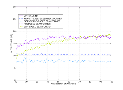
Figure 2: Output SINR versus training sample size $K$ for fixed $\rm{SNR}=20$ dB and $\rm{INR}=30$ dB .

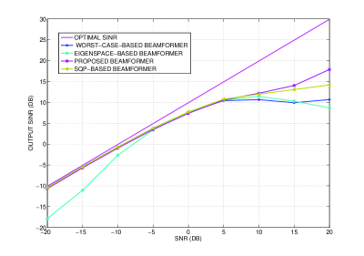
Figure 3: Output SINR versus SNR for training data size of $K=30$ and $\rm{INR}=30$ dB.

In the first example, we consider the case when the actual desired signal steering vector is known exactly. Even in this case, the presence of the signal of interest in the training data can substantially reduce the convergence rates of adaptive beamforming algorithms as compared to the signal-free training data case [8]. In Fig. 2, the mean output SINRs for the aforementioned methods are illustrated versus the number of training snapshots for the fixed single-sensor $\rm{SNR}=20$ dB. Fig. 3 displays the mean output SINR of the same methods versus the SNR for fixed training data size of $K=30$. It can be seen from these figures that the proposed beamforming technique outperforms the other techniques even in the case of exactly known signal steering vector. It is especially true for small sample size.

VI-B Example 2: Signal Spatial Signature Mismatch Due to Wavefront Distortion.

In the second example, we consider the situation when the signal steering vector is distorted by wave propagation effects in an inhomogeneous medium. Independent-increment phase distortions are accumulated by the components of the presumed steering vector. It is assumed that the phase increments remain fixed in each simulation run and are independently chosen from a Guassian random generator with zero mean and variance $0.04$.

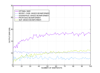
Figure 4: Output SINR versus training sample size $K$ for fixed $\rm{SNR}=20$ dB and $\rm{INR}=30$ dB.

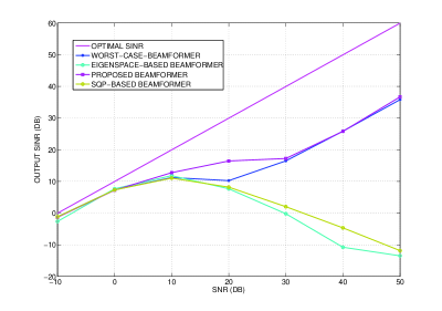
Figure 5: Output SINR versus SNR for training data size of $K=30$ and $\rm{INR}=30$ dB.

The performance of the methods tested is shown versus the number of training snapshots for fixed single-sensor SNR$=20$ dB in Fig. 4 and versus the SNR for fixed training data size $K=30$ in Fig. 5. It can be seen from these figures that the proposed beamforming technique outperforms all other beamforming techniques. Interestingly, it outperforms the eigenspace-based beamformer even at high SNR. This performance improvement compared to the eigenspace-based beamformer can be attributed to the fact that the knowledge of sector which includes the desired signal steering vector is used in the proposed beamforming technique. Fig. 5 also illustrates the case when SNR$\gg$INR where INR stands for interference-to-noise ratio. This case aims to illustrate the situation when SIR$\rightarrow\infty$. As it can be expected, the proposed and the worst-case-based methods perform almost equivalently.

VI-C Example 3: Signal Spatial Signature Mismatch Due to Coherent Local Scattering

The third example corresponds to the scenario of coherent local scattering [34]. In this case, the desired signal steering vector is distorted by local scattering effects so that the presumed signal steering vector is a plane wave, whereas the actual steering vector is formed by five signal paths as

$$\mathbf{a}=\mathbf{p}+\sum_{i=1}^{4}e^{j\psi_{i}}\mathbf{b}(\theta_{i})$$ (55)

where $\mathbf{p}$ corresponds to the direct path and $\mathbf{b}(\theta_{i}),\ i=1,2,3,4$ correspond to the coherently scattered paths. We model the $i$th path $\mathbf{b}(\theta_{i})$ as a a plane wave impinging on the array from the direction $\theta_{i}$. The angles $\theta_{i}$, $i=1,2,3,4$ are independently drawn in each simulation run from a uniform random generator with mean $3^{\circ}$ and standard deviation $1^{\circ}$. The parameters $\psi_{i},\ \ i=1,2,3,4$ represent path phases that are independently and uniformly drawn from the interval $[0,2\pi]$ in each simulation run. Note that $\theta_{i}$ and $\psi_{i},\ \ i=1,2,3,4$ change from run to run but do not change from snapshot to snapshot.

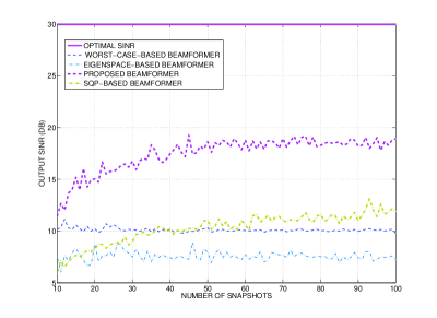
Figure 6: Output SINR versus training sample size $K$ for fixed $\rm{SNR}=20$ dB and $\rm{INR}=30$ dB.

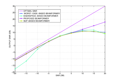
Figure 7: Output SINR versus SNR for training data size of $K=30$ and $\rm{INR}=30$ dB.

Fig. 6 displays the performance of all four methods tested versus the number of training snapshots $K$ for fixed single-sensor $\rm{SNR}=20$ dB. Note that the SNR in this example is defined by taking into account all signal paths. The performance of the same methods versus SNR for the fixed training data size $K=30$ is displayed in Fig. 7. Similar to the previous example, the proposed beamformer significantly outperforms other beamformers due to its ability to estimate the actual steering vector with a hight accuracy.

VII Conclusion

A new approach to robust adaptive beamforming in the presence of signal steering vector errors has been developed. According to this approach, the actual steering vector is first estimated using its presumed (prior) value, and then this estimate is used to find the optimal beamformer weight vector. The problem of signal steering vector estimation belongs to the class of homogeneous QCQP problems. It has been shown that this problem can be solved using the SDP relaxation technique or the strong duality theory and the exact solution for the signal steering vector can be found efficiently or even in some cases in closed-form. As compared to another well-known robust adaptive beamforming method based on the signal steering vector correction/estimation, that is, the eigespace-based method, the proposed technique does not suffer from the subspace swap phenomenon since it does not use eigenvalue decomposition of the sample covariance matrix. Moreover, it does not require any knowledge on the number of interferences. As compared to the well-known worst-case-based and probabilistically-constrained robust adaptive beamformers, the proposed technique does not use any design parameters of non-unique choice. Our simulation results demonstrate the superior performance for the proposed method over the aforementioned robust adaptive beamforming methods for several frequently encountered types of signal steering vector errors.

Appendix

Proof of Theorem 1

Let $\hat{\mathbf{a}}$ be a feasible point for the original problem (15)–(17). It is straightforward to see that $\mathbf{A}=\hat{\mathbf{a}}\hat{\mathbf{a}}^{H}$ is also a feasible point for the relaxed problem (25)–(28). Thus, the necessity statement of the theorem follows trivially.

Let us now prove sufficiency. Let $\mathbf{A}=\sum_{i=1}^{M}\lambda_{i}\mathbf{b}_{i}\mathbf{b}_{i}^{H}$ be a feasible point for the relaxed problem (25)–(28), where $\lambda_{i}$ and $\mathbf{b}_{i}$, $i=1,\cdots,M$ are, respectively, the eigenvalues and eigenvectors of $\mathbf{A}$. Also let $l=\arg\min_{i}{\mathbf{b}_{i}^{H}\tilde{\mathbf{C}}\mathbf{b}_{i}}$ and $\hat{\mathbf{a}}=\sqrt{M}\mathbf{b}_{l}$. Then the following holds

$$\hat{\mathbf{a}}^{H}\hat{\mathbf{a}}=M\mathbf{b}_{l}^{H}\mathbf{b}_{l}=M$$ (56)

and the constraint (17) is satisfied.

Moreover, we can write that

$$\hat{\mathbf{a}}^{H}\tilde{\mathbf{C}}\hat{\mathbf{a}}=M\mathbf{b}_{l}^{H}\tilde{\mathbf{C}}\mathbf{b}_{l}=\left(\sum_{i=1}^{M}\lambda_{i}\right)\mathbf{b}_{l}^{H}\tilde{\mathbf{C}}\mathbf{b}_{l}$$ (57)

where $\sum_{i=1}^{M}\lambda_{i}=Tr(\mathbf{A})=M$. Using the following inequality

$$\left(\sum_{i=1}^{M}\lambda_{i}\right)\mathbf{b}_{l}^{H}\tilde{\mathbf{C}}\mathbf{b}_{l}\leq\sum_{i=1}^{M}\lambda_{i}\mathbf{b}_{i}^{H}\tilde{\mathbf{C}}\mathbf{b}_{i}$$ (58)

and (57), we obtain that

$$\hat{\mathbf{a}}^{H}\tilde{\mathbf{C}}\hat{\mathbf{a}}\leq\sum_{i=1}^{M}\lambda_{i}\mathbf{b}_{i}^{H}\tilde{\mathbf{C}}\mathbf{b}_{i}.$$ (59)

The right hand side of (59) can be further rewritten as

$$\sum_{i=1}^{M}\lambda_{i}\mathbf{b}_{i}^{H}\tilde{\mathbf{C}}\mathbf{b}_{i}=\sum_{i=1}^{M}\lambda_{i}Tr(\tilde{\mathbf{C}}\mathbf{b}_{i}\mathbf{b}_{i}^{H}).$$ (60)

Using the property of the trace that a sum of traces is equal to the trace of a sum, we obtain that

$$\sum_{i=1}^{M}\lambda_{i}Tr(\tilde{\mathbf{C}}\mathbf{b}_{i}\mathbf{b}_{i}^{H})=Tr\left(\tilde{\mathbf{C}}\sum_{i=1}^{K}(\lambda_{i}\mathbf{b}_{i}\mathbf{b}_{i}^{H})\right).$$ (61)

Moreover, since $\sum_{i=1}^{K}\lambda_{i}\mathbf{b}_{i}\mathbf{b}_{i}^{H}=\mathbf{A}$, we have

$$\sum_{i=1}^{M}\lambda_{i}\mathbf{b}_{i}^{H}\tilde{\mathbf{C}}\mathbf{b}_{i}=Tr\left(\tilde{\mathbf{C}}\sum_{i=1}^{K}\lambda_{i}\mathbf{b}_{i}\mathbf{b}_{i}^{H}\right)=Tr(\tilde{\mathbf{C}}\mathbf{A}).$$ (62)

Substituting (62) in the left hand side of (59), we finally obtain that

$$\hat{\mathbf{a}}^{H}\tilde{\mathbf{C}}\hat{\mathbf{a}}\leq Tr(\tilde{\mathbf{C}}\mathbf{A})\leq\Delta_{0}.$$ (63)

Therefore, the constraint (17) is also satisfied and, thus, $\mathbf{a}=\sqrt{M}\mathbf{b}_{l}$ is a feasible point for (15)–(17) that completes the proof. $\square$

Proof of Theorem 2

Let $\mathbf{A}^{*}$ be the optimal minimizer of the relaxed problem (25)–(28), and its rank be $r$. Consider the following decomposition of $\mathbf{A}^{*}$

$$\mathbf{A}^{*}=\mathbf{Y}\mathbf{Y}^{H}$$ (64)

where $\mathbf{Y}$ is an $N\times r$ complex valued matrix. It is trivial that if the rank of the optimal minimizer $\mathbf{A}^{*}$ of the relaxed problem (25)–(28) equals one, then $\mathbf{Y}$ is the optimal minimizer of the original problem (15)–(17). Thus, it is assumed in the following that $r>1$.

We start by considering the following auxiliary optimization problem

$$\min_{\mathbf{G}} Tr(\hat{\mathbf{R}}^{-1}\mathbf{Y}\mathbf{G}\mathbf{Y}^{H})$$ (65)

$${\rm subject\ to} Tr(\mathbf{Y}\mathbf{G}\mathbf{Y}^{H})=M$$ (68)

$$Tr(\tilde{\mathbf{C}}\mathbf{Y}\mathbf{G}\mathbf{Y}^{H})=Tr(\tilde{\mathbf{C}}\mathbf{A}^{*})$$

$$\mathbf{G}\succeq 0$$

where $\mathbf{G}$ is an $r\times r$ Hermitian matrix. The matrix $\mathbf{A}$ in (25)–(28) can be expressed as a function of the matrix $\mathbf{G}$ in (65)–(68) as $\mathbf{A}(\mathbf{G})=\mathbf{Y}\mathbf{G}\mathbf{Y}^{H}$. Moreover, it can be easily shown that if $\mathbf{G}$ is a positive semi-definite matrix, then $\mathbf{A}(\mathbf{G})$ is also a positive semi-definite matrix. In addition, if $\mathbf{G}$ is a feasible solution of (65)–(68), $\mathbf{A}(\mathbf{G})$ is also a feasible solution of (25)–(28). The latter is true because $\mathbf{A}(\mathbf{G})$ is a positive semi-definite matrix and it satisfies the constraints $Tr(\mathbf{A}(\mathbf{G}))=M$ and $Tr(\tilde{\mathbf{C}}\,\mathbf{A}(\mathbf{G}))=Tr(\tilde{\mathbf{C}}\mathbf{A}^{*})\leq\Delta_{0}$. This implies that the minimum value of the problem (65)–(68) is greater than or equal to the minimum value of the problem (25)–(28).

It is then easy to verify that $\mathbf{G}^{*}=\mathbf{I}_{r}$ is a feasible point of the auxiliary optimization problem (65)–(68). Moreover, the fact that $Tr(\hat{\mathbf{R}}^{-1}\mathbf{Y}\mathbf{G}^{*}\mathbf{Y}^{H})=Tr(\hat{\mathbf{R}}^{-1}\mathbf{A}^{*})\triangleq\beta$ (here $\beta$ denotes the minimum value of the relaxed problem (25)–(28)) together with the fact that the minimum value of the auxiliary problem (65)–(68) is greater than or equal to $\beta$, implies that $\mathbf{G}^{*}=\mathbf{I}_{r}$ is the optimal solution of the auxiliary problem (65)–(68).

Next, we show that if $\mathbf{G}^{\prime}$ is a feasible solution of (65)–(68), then it is also an optimum minimizer of (65)–(68). Therefore, $\mathbf{A}(\mathbf{G}^{\prime})=\mathbf{Y}\mathbf{G}^{\prime}\mathbf{Y}^{H}$ is also an optimum minimizer of (25)–(28). Towards this end, let us consider the following dual to (65)–(68) problem

$$\max_{\mathbf{\nu}_{1},\nu_{2},\mathbf{Z}} \nu_{1}M+\nu_{2}Tr(\tilde{\mathbf{C}}\mathbf{A}^{*})$$ (69)

$${\rm subject\ to} \mathbf{Y}^{H}\hat{\mathbf{R}}^{-1}\mathbf{Y}-\nu_{1}\mathbf{Y}^{H}\mathbf{Y}-\nu_{2}\mathbf{Y}^{H}\tilde{\mathbf{C}}\mathbf{Y}\succeq\mathbf{Z}$$ (71)

$$\mathbf{Z}\succeq 0$$

where $\nu_{1}$ and $\nu_{2}$ are the Lagrange multipliers associated with the constraints (68) and (68), respectively, and $\mathbf{Z}$ is an $r\times r$ Hermitian matrix. Note that the optimization problem (65)–(68) is convex. Moreover, it satisfies the Slater’s conditions because, as it was mentioned, the positive definite matrix $\mathbf{G}=\mathbf{I}_{r}$ is a feasible point for (65)–(68). Thus, the strong duality between (65)–(68) and (69)–(71) holds.

Let $\nu_{1}^{*},\ \nu_{2}^{*}$, and $\mathbf{Z}^{*}$ be one possible optimal solution of the dual problem (69)–(71). Since strong duality holds, $\nu_{1}^{*}M+\nu_{2}^{*}Tr(\tilde{\mathbf{C}}\mathbf{A}^{*})=\beta$ and $\mathbf{I}_{r}$ is an optimal solution of the primal problem (65)–(68). Moreover, the complementary slackness condition implies that

$$Tr(\mathbf{G}^{*}\mathbf{Z}^{*})=Tr(\mathbf{Z}^{*})=0.$$ (72)

Since $\mathbf{Z}^{*}$ has to be a positive semi-definite matrix, the condition (72) implies that $\mathbf{Z}^{*}=0$. Then it follows from (71) that

$$\mathbf{Y}^{H}\hat{\mathbf{R}}^{-1}\mathbf{Y}\succeq\nu_{1}^{*}\mathbf{Y}^{H}\mathbf{Y}+\nu_{2}^{*}\mathbf{Y}^{H}\tilde{\mathbf{C}}\mathbf{Y}.$$ (73)

Using the fact that $\mathbf{Y}^{H}\mathbf{Y}$ and $\mathbf{Y}^{H}\tilde{\mathbf{C}}\mathbf{Y}$ are positive semi-definite matrices, it can be easily verified that the constraint (73) is active, i.e., it is satisfied as equality for optimal $\nu_{1}^{*}$ and $\nu_{2}^{*}$. Therefore, we can write that

$$\mathbf{Y}^{H}\hat{\mathbf{R}}^{-1}\mathbf{Y}=\nu_{1}^{*}\mathbf{Y}^{H}\mathbf{Y}+\nu_{2}^{*}\mathbf{Y}^{H}\tilde{\mathbf{C}}\mathbf{Y}.$$ (74)

Let $\mathbf{G}^{\prime}$ be another feasible solution of (65)–(68) different from $\mathbf{I}_{r}$. Then the following conditions must hold

$$Tr(\mathbf{Y}^{H}\mathbf{Y}\mathbf{G}^{\prime})=M$$ (75)

$$Tr(\mathbf{Y}^{H}\tilde{\mathbf{C}}\mathbf{Y}\mathbf{G}^{\prime})=Tr(\tilde{\mathbf{C}}\mathbf{A}^{*})$$ (76)

$$\mathbf{G}^{\prime}\succeq 0.$$ (77)

Multiplying both sides of the equation (74) by $\mathbf{G}^{\prime}$, we obtain

$$\mathbf{Y}^{H}\hat{\mathbf{R}}^{-1}\mathbf{Y}\mathbf{G}^{\prime}=\nu_{1}^{*}\mathbf{Y}^{H}\mathbf{Y}\mathbf{G}^{\prime}+\nu_{2}^{*}\mathbf{Y}^{H}\tilde{\mathbf{C}}\mathbf{Y}\mathbf{G}^{\prime}.$$ (78)

Moreover, taking the trace of the right hand and left hand sides of (78), we have

$$Tr(\mathbf{Y}^{H}\hat{\mathbf{R}}^{-1}\mathbf{Y}\mathbf{G}^{\prime})\!\!\! = \!\!\!\nu_{1}^{*}Tr(\mathbf{Y}^{H}\mathbf{Y}\mathbf{G}^{\prime})+\nu_{2}^{*}Tr(\mathbf{Y}^{H}\tilde{\mathbf{C}}\mathbf{Y}\mathbf{G}^{\prime})$$ (79)

$$= \!\!\!\nu_{1}^{*}M+\nu_{2}^{*}Tr(\tilde{\mathbf{C}}\mathbf{A}^{*})=\beta.$$

This implies that $\mathbf{G}^{\prime}$ is also an optimal solution of the problem (65)–(68). Therefore, every feasible solution of (65)–(68) is also an optimal solution.

Finally, we show that there exists a feasible solution of (65)–(68) whose rank is one. As it has been proved above, such feasible solution will also be optimal. Let $\mathbf{G}=\mathbf{v}\mathbf{v}^{H}$. Thus, we are interested in finding such $\mathbf{v}$ that

$$Tr(\mathbf{Y}^{H}\mathbf{Y}\mathbf{v}\mathbf{v}^{H})=M$$ (80)

$$Tr(\mathbf{Y}^{H}\tilde{\mathbf{C}}\mathbf{Y}\mathbf{v}\mathbf{v}^{H})=Tr(\tilde{\mathbf{C}}\mathbf{A}^{*}).$$ (81)

Equivalently, the conditions (80) and (81) can be rewritten as

$$\mathbf{v}^{H}\mathbf{Y}^{H}\mathbf{Y}\mathbf{v}=M$$ (82)

$$\mathbf{v}^{H}\mathbf{Y}^{H}\tilde{\mathbf{C}}\mathbf{Y}\mathbf{v}=Tr(\tilde{\mathbf{C}}\mathbf{A}^{*}).$$ (83)

We can further write that

$$\frac{1}{M}\mathbf{v}^{H}\mathbf{Y}^{H}\mathbf{Y}\mathbf{v}=1$$ (84)

$$\mathbf{v}^{H}\frac{\mathbf{Y}^{H}\tilde{\mathbf{C}}\mathbf{Y}}{Tr(\tilde{\mathbf{C}}\mathbf{A}^{*})}\mathbf{v}=1.$$ (85)

Moreover, equating the left hand side of (84) to the left hand side of (85), we obtain that

$$\frac{1}{M}\mathbf{v}^{H}\mathbf{Y}^{H}\mathbf{Y}\mathbf{v}=\mathbf{v}^{H}\frac{\mathbf{Y}^{H}\tilde{\mathbf{C}}\mathbf{Y}}{Tr(\tilde{\mathbf{C}}\mathbf{A}^{*})}\mathbf{v}.$$ (86)

Subtracting the left hand side of (86) from its right hand side, we also obtain that

$$\mathbf{v}^{H}\left(\frac{1}{M}\mathbf{Y}^{H}\mathbf{Y}-\frac{\mathbf{Y}^{H}\tilde{\mathbf{C}}\mathbf{Y}}{Tr(\tilde{\mathbf{C}}\mathbf{A}^{*})}\right)\mathbf{v}=\mathbf{v}^{H}\mathbf{D}\mathbf{v}=0.$$ (87)

Considering the fact that $Tr(\mathbf{D})=0$, the vector $\mathbf{v}$ can be chosen as the sum of the eigenvectors of the matrix $\mathbf{D}$ in (29). Note that $\mathbf{v}$ can be chosen proportional to the sum of the eigenvectors of the matrix $\mathbf{D}$ such that $\mathbf{v}^{H}\mathbf{Y}^{H}\mathbf{Y}\mathbf{v}=M$ is satisfied. It will also imply that $\mathbf{v}^{H}{\mathbf{Y}^{H}\tilde{\mathbf{C}}\mathbf{Y}}\mathbf{v}=Tr(\tilde{\mathbf{C}}\mathbf{A}^{*})$ and, thus, (82) and (83) are satisfied.

So far we have found a rank one solution for the auxiliary optimization problem (68)–(68), that is, $\mathbf{G}=\mathbf{v}\mathbf{v}^{H}$. Since $\mathbf{G}=\mathbf{v}\mathbf{v}^{H}$ is the optimal solution of the auxiliary problem (68)–(68), then $\mathbf{Y}\mathbf{G}\mathbf{Y}^{H}=(\mathbf{Y}\mathbf{v})(\mathbf{Y}\mathbf{v})^{H}$ is the optimal solution of the relaxed problem (25)–(28). Moreover, since the solution $(\mathbf{Y}\mathbf{v})(\mathbf{Y}\mathbf{v})^{H}$ is rank-one, $\mathbf{Y}\mathbf{v}$ is the optimal solution of the original optimization problem (15)–(17). This completes the proof. $\hfill\square$

Proof of Theorem 3

Let $\mathbf{A}^{*}$ be one optimal solution of the problem (25)–(28) whose rank $r$ is greater than one. Using the rank-one decomposition of Hermitian matrices [35], the matrix $\mathbf{A}^{*}$ can be written as

$$\mathbf{A}^{*}=\sum_{j=1}^{r}\mathbf{z}_{j}\mathbf{z}_{j}^{H}$$ (88)

where

$$\mathbf{z}_{j}^{H}\mathbf{z}_{j}=\frac{1}{r}Tr(\mathbf{A}^{*})=\frac{M}{r},\quad j=1,\ldots,r$$ (89)

$$\mathbf{z}_{j}^{H}\tilde{\mathbf{C}}\mathbf{z}_{j}=\frac{1}{r}Tr(\tilde{\mathbf{C}}\mathbf{A}^{*}),\quad j=1,\ldots,r.$$ (90)

Let us show that the terms $\mathbf{z}_{j}^{H}\hat{\mathbf{R}}^{-1}\mathbf{z}_{j}$, $j=1,\ldots,r$ are equal to each other for all $j=1,\ldots,r$. We prove it by contradiction assuming first that there exist such $\mathbf{z}_{m}$ and $\mathbf{z}_{n}$, $m\neq n$ that $\mathbf{z}_{m}^{H}\hat{\mathbf{R}}^{-1}\mathbf{z}_{m}<\mathbf{z}_{n}^{H}\hat{\mathbf{R}}^{-1}\mathbf{z}_{n}$. Let the matrix $\mathbf{A}^{*}_{0}$ be constructed as $\mathbf{A}^{*}_{0}=\mathbf{A}^{*}-\mathbf{z}_{n}\mathbf{z}_{n}^{H}+\mathbf{z}_{m}\mathbf{z}_{m}^{H}$. It is easy to see that $Tr(\mathbf{A}^{*})=Tr(\mathbf{A}^{*}_{0})$ and $Tr(\tilde{\mathbf{C}}\mathbf{A}^{*})=Tr(\tilde{\mathbf{C}}\mathbf{A}^{*}_{0})$, which means that $\mathbf{A}^{*}_{0}$ is also a feasible solution of the problem (25)–(28). However, based on our assumption that $\mathbf{z}_{m}^{H}\hat{\mathbf{R}}^{-1}\mathbf{z}_{m}<\mathbf{z}_{n}^{H}\hat{\mathbf{R}}^{-1}\mathbf{z}_{n}$, it can be concluded that $Tr(\hat{\mathbf{R}}^{-1}\mathbf{A}^{*}_{0})<Tr(\hat{\mathbf{R}}^{-1}\mathbf{A}^{*}_{0})$ that is obviously a contradiction. Thus, all terms $\mathbf{z}_{j}^{H}\hat{\mathbf{R}}^{-1}\mathbf{z}_{j}$, $j=1,\ldots,r$ must take the same value. Using this fact together with the equations (89) and (90), we can conclude that $r\mathbf{z}_{j}\mathbf{z}_{j}^{H}$ for any $j=1,\ldots,r$ is the optimal solution of the relaxed optimization problem (25)–(28) which has rank one. Thus, the optimal solution of the original problem (15)–(17) is $\sqrt{r}\mathbf{z}_{j}$ for any $j=1,\ldots,r$. Since the vectors $\mathbf{z}_{j}$, $j=1,...,r$ in (88) are linearly independent and each of them gives an optimal solution to the problem (15)–(17), we conclude that the optimal solution to (15)–(17) is not unique up to a phase rotation. However, it contradicts the assumption that the optimal solution of (15)–(17) is unique up to a phase rotation. Thus, the optimal solution $\mathbf{A}^{*}$ to the relaxed problem (25)–(28) must be rank-one. This completes the proof. $\hfill\square$

References

- [1] H. L. Van Trees, Optimum Array Processing. New York: Wiley, 2002.
- [2] I. S. Reed, J. D. Mallett, and L. E. Brennan, “Rapid convergence rate in adaptive arrays,” IEEE Trans. Aerosp. Electron. Syst., vol. 10, pp. 853 -863, Nov. 1974.
- [3] L. J. Griffiths and C. W. Jim, “An alternative approach to linearly constrained adaptive beamforming,” IEEE Trans. Antennas Propagat., vol. 30, pp. 27 -34, Jan. 1982.
- [4] E. K. Hung and R. M. Turner, “A fast beamforming algorithm for large arrays,” IEEE Trans. Aerosp. Electron. Syst., vol. 19, pp. 598 -607, July 1983.
- [5] A. B. Gershman, “Robust adaptive beamforming in sensor arrays,” Int. J. Electron. Commun., vol. 53, pp. 305 -314, Dec. 1999.
- [6] H. Cox, R. M. Zeskind, and M. H. Owen, “Robust adaptive beamforming,” IEEE Trans. Acoust., Speech, Signal Processing, vol. ASSP-35, pp. 1365 -1376, Oct. 1987.
- [7] Y. I. Abramovich, “Controlled method for adaptive optimization of filters using the criterion of maximum SNR,” Radio Eng. Electron. Phys., vol. 26, pp. 87 -95, Mar. 1981.
- [8] D. D. Feldman and L. J. Griffiths, “A projection approach to robust adaptive beamforming,” IEEE Trans. Signal Processing, vol. 42, pp. 867- 876, Apr. 1994.
- [9] L. Chang and C. C. Yeh, “Performance of DMI and eigenspace-based beamformers,” IEEE Trans. Antennas Propagat., vol. 40, pp. 1336 -1347, Nov. 1992.
- [10] J. K. Thomas, L. L. Scharf, and D. W. Tufts, “The probability of a subspace swap in the SVD,” IEEE Trans. Signal Processing, vol. 43, pp. 730 -736, Mar. 1995.
- [11] S. A. Vorobyov, A. B. Gershman, Z.-Q. Luo,“Robust adaptive beamforming using worst-case performance optimization: A solution to the signal mismatch problem,” IEEE Trans. Signal Processing, vol. 51, pp. 313–324, Feb. 2003.
- [12] S. A. Vorobyov, A. B. Gershman, Z.-Q. Luo, and N. Ma, “Adaptive beamforming with joint robustness against mismatched signal steering vector and interference nonstationarity,” IEEE Signal Processing Lett., vol. 11, pp. 108- 111, Feb. 2004.
- [13] J. Li, P. Stoica, and Z. Wang, “On robust Capon beamforming and diagonal loading,” IEEE Trans. Signal Process., vol. 51, pp. 1702- 1715, July 2003.
- [14] R. G. Lorenz and S. P. Boyd, “Robust minimum variance beamforming,” IEEE Trans. Signal Process., vol. 53, pp. 1684- 1696, May 2005.
- [15] S. Shahbazpanahi, A. B. Gershman, Z.-Q. Luo, and K. M. Wong, “Robust adaptive beamforming for general-rank signal models,” IEEE Trans. Signal Process., vol. 51, pp. 2257 -2269, Sep. 2003.
- [16] S. A. Vorobyov, Y. Rong, and A. B. Gershman, “Robust adaptive beamforming using probability-constrained optimization,” in Proc. IEEE SSP Workshop, Bordeaux, France, July 2005, pp. 934–939.
- [17] S. A. Vorobyov, H. Chen, and A. B. Gershman, “On the relationship between robust minimum variance beamformers with probabilistic and worst-case distrortionless response constraints,” IEEE Trans. Signal Processing, vol. 56, pp. 5719–5724, Nov. 2008.
- [18] S. A. Vorobyov, A. B. Gershman, and Y. Rong, “On the relationship between the worst-case optimization-based and probability-constrained approaches to robust adaptive beamforming,” in Proc. IEEE ICASSP, Honolulu, HI, Apr. 2007, pp. 977- 980.
- [19] A. Hassanien, S. A. Vorobyov, and K. M. Wong, “Robust adaptive beamforming using sequential quadratic programming,” in Proc. IEEE ICASSP, Las Vegas, NV, Apr. 2008, pp. 2345–2348.
- [20] A. Hassanien, S. A. Vorobyov, and K. M. Wong, “Robust adaptive beamforming using sequential programming: An iterative solution to the mismatch problem,” IEEE Signal Processing Lett., vol. 15, pp. 733–736, 2008.
- [21] J. Li, P. Stoica, and Z. Wang, “Doubly constrained robust capon beamformer,” IEEE Trans. Signal Processing, vol. 52, pp. 2407–2423, Sept. 2004.
- [22] S. Zhang and Y. Huang, “Complex quadratic optimization and semidefinite programming,” SIAM J. Optim., vol. 16, no. 3, pp. 871–890, 2006.
- [23] Z.-Q. Luo, W.-K. Ma, A. M.-C. So, Y. Ye, and S. Zhang, “Semidefinite relaxation of quadratic optimization problems,” IEEE Signal Processing Magazin, vol. 27, no. 3, pp. 20–34, May 2010.
- [24] Y. S. Nesterov, “Semidefinite relaxation and nonconvex quadratic optimization,” Optim. Methods Softw., vol. 9, no. 1–3, pp. 141–160, 1998.
- [25] K. T. Phan, S. A. Vorobyov, N. D. Sidiropoulos, and C. Tellambura, “Spectrum sharing in wireless networks via QoS-aware secondary multicast beamforming,” IEEE Trans. Signal Processing, vol. 57, pp.2323–2335, June 2009.
- [26] S. Zhang, “Quadratic maximization and semidefinite relaxation,” Math. Program. A, vol. 87, pp. 453 -465, 2000.
- [27] Z.-Q. Luo, N. D. Sidiropoulos, P. Tseng, and S. Zhang, “Approximation bounds for quadratic optimization with homogeneous quadratic constraints,” SIAM J. Optim., vol. 18, no. 1, pp. 1–28, Feb. 2007.
- [28] J. F. Sturm, “Using SeDuMi 1.02, a MATLAB toolbox for optimization over symmetric cones,” Optim. Meth. Softw., vol. 11 12, pp. 625 -653, Aug. 1999. Available [Online]: http://sedumi.ie.lehigh.edu/
- [29] A. B. Gershman, Z.-Q. Luo, and S. Shahbazpanahi, “Robust adaptive beamforming based on worst-case performance optimization,” in Robust Adaptive Beamforming, P. Stoica and J. Li, Eds. Hoboken, NJ: Wiley, 2006, pp. 49 -89.
- [30] L. Lei, J. P. Lie, A. B. Gershman, and C. M. S. See, “Robust adaptive beamforming in partly calibrated sparse sensor arrays,“ IEEE Trans. Signal Processing, vol. 58, pp. 1661–1667, Mar. 2010.
- [31] A. Beck and Y. C. Eldar, “Strong duality in nonconvex quadratic optimization with two quadratic constraints,” SIAM J. Optimization, vol. 17, no. 3, pp. 844–860, 2006.
- [32] A. Beck and Y. C. Eldar, “Doubly constrained robust Capon beamformer with ellipsoidal uncertainty sets,” IEEE Trans. Signal Processing, vol. 55, pp. 753–758, Feb. 2007.
- [33] Available [Online]: http://cvxr.com/cvx/
- [34] J. Goldberg and H. Messer, “Inherent limitations in the localization of a coherently scattered source,” IEEE Trans. Signal Processing, vol. 46, pp. 3441 -3444, Dec. 1998.
- [35] Y. Huang and S. Zhang, “Complex Matrix Decomposition and Quadratic Programming,” Mathematics of Operations Research, vol. 32, no. 3, pp. 758–768, Aug. 2007.