BU-HEPP-10-04
Jul., 2010

An Estimate of $\Lambda$ in Resummed Quantum Gravity in the Context of Asymptotic Safety^†

B.F.L. Ward
Department of Physics,
Baylor University, Waco, Texas, 76798-7316, USA

Abstract

We show that, by using recently developed exact resummation techniques based on the extension of the methods of Yennie, Frautschi and Suura to Feynman’s formulation of Einstein’s theory, we get quantum field theoretic descriptions for the UV fixed-point behaviors of the dimensionless gravitational and cosmological constants postulated by Weinberg. Connecting our work to the attendant phenomenological asymptotic safety analysis of Planck scale cosmology by Bonanno and Reuter, we estimate the value of the cosmological constant $\Lambda$. We find the encouraging estimate $\rho_{\Lambda}\equiv\frac{\Lambda}{8\pi G_{N}}\simeq(2.4\times 10^{-3}eV)^{4}$. While this numerical value is close to recent experimental observations, we caution the reader that the estimate involves a number of model parameters that still possess significant levels of uncertainty, such as the value of the transition time between the Planck scale cosmology era and the Friedmann-Robertson-Walker radiation dominated era, where our current understanding allows for at least two orders of magnitude in its uncertainty and this would change our estimate of $\rho_{\Lambda}$ by at least four orders of magnitude. We discuss such theoretical uncertainties as well. We show why GUT and EW scale vacuum energies from spontaneous symmetry breaking are suppressed in our approach to the estimation of $\rho_{\Lambda}$. As a bonus, we show how our estimate constrains susy GUTS.

• Work partly supported by NATO Grant PST.CLG.980342.

1 Introduction

In Ref. [1], Weinberg suggested that the general theory of relativity may have a non-trivial UV fixed point, with a finite dimensional critical surface in the UV limit, so that it would be asymptotically safe with an S-matrix that depends on only a finite number of observable parameters. In Refs. [2, 3, 4, 5, 6, 7], strong evidence has been calculated using Wilsonian [8] field-space exact renormalization group methods to support Weinberg’s asymptotic safety hypothesis for the Einstein-Hilbert theory. As we review briefly below, in a parallel but independent development [9, 10, 11, 12, 13, 14, 15, 16, 17, 18], we have shown [19] that the extension of the amplitude-based, exact resummation theory of Ref. [20, 21] to the Einstein-Hilbert theory leads to UV-fixed-point behavior for the dimensionless gravitational and cosmological constants, but with the added bonus that the resummed theory is actually UV finite when expanded in the resummed propagators and vertices to any finite order in the respective improved loop expansion. We have called the resummed theory resummed quantum gravity. More recently, more evidence for Weinberg’s asymptotic safety behavior has been calculated using causal dynamical triangulated lattice methods in Ref. [22]. At this point, there is no known inconsistency between our analysis and those of the Refs. [2, 3, 4, 5, 6, 7, 22].

We need to stress that the results in Refs. [2, 3, 4, 5, 6, 7], while impressive, involve cut-offs which remain in the results to varying degrees even for products such as that for the UV limits of the dimensionless gravitational and cosmological constants. In addition, the results in Refs. [2, 3, 4, 5, 6, 7] retain some mild dependence on gauge parameters, again even for the product of the UV limits of the dimensionless gravitational and cosmological constants. Accordingly, henceforward, we refer to the approach in Refs. [2, 3, 4, 5, 6, 7] as the ’phenomenological’ asymptotic safety approach. What can be said is that dependencies are mild enough that the existence of the non-Gaussian UV fixed point found in these references is probably a physical result. But, until a rigorously cut-off independent and gauge invariant calculation corroborates these results, we cannot consider them final. Our approach offers such a calculation, as our results are both gauge invariant and cut-off independent. The results from Refs. [22], involving, as they most certainly do, lattice constant-type artifact issues, are also only an indication of what the true continuum limit might realize – they too need to be corroborated by a rigorous calculation without the issues of finite size and other possible lattice artifacts to be considered final. Again, our approach offers an answer to these issues. The stage is therefore prepared for us to try to make contact with experiment, as such contact is the ultimate purpose of theoretical physics.

Toward this end, we note that, in Refs. [24, 25], it has been argued that the attendant phenomenological asymptotic safety approach in Refs. [2, 3, 4, 5, 6, 7] to quantum gravity may indeed provide a realization of the successful inflationary model [27, 28] of cosmology without the need of the as yet unseen inflaton scalar field: the attendant UV fixed point solution allows one to develop Planck scale cosmology that joins smoothly onto the standard Friedmann-Walker-Robertson classical descriptions so that then one arrives at a quantum mechanical solution to the horizon, flatness, entropy and scale free spectrum problems. In Ref. [19], we have shown that, in the new resummed theory [9, 10, 11, 12, 13, 14, 15, 16, 17, 18] of quantum gravity, we recover the properties as used in Refs. [24, 25] for the UV fixed point of quantum gravity with the added results that we get “first principles” predictions for the fixed point values of the respective dimensionless gravitational and cosmological constants in their analysis. In what follows here, we carry the analysis one step further and arrive at an estimate for the observed cosmological constant $\Lambda$ in the context of the Planck scale cosmology of Refs. [24, 25]. We comment on the reliability of the result as well, as it will be seen already to be relatively close to the observed value [29, 30]. While we obviously do not want to overdo the closeness to the experimental value, we do want to argue that this again gives, at the least, some more credibility to the new resummed theory as well as to the methods in Refs. [2, 3, 4, 5, 6, 7, 22]. More reflections on the attendant implications of the latter credibility in the search for an experimentally testable union of the original ideas of Bohr and Einstein will be taken up elsewhere [31].

The discussion is organized as follows. We start by recapitulating the Planck scale cosmology presented phenomenologically in Refs. [24, 25]. This is done in the next section. We then review our results in Ref. [19] for the dimensionless gravitational and cosmological constants at the UV fixed point. In the course of this latter review, which is done in Section 3, we give a new proof of the UV finiteness of the resummed quantum gravity theory for the sake of completeness. In Section 4, we then combine the Planck scale cosmology scenario in Refs. [24, 25] with our results to estimate the observed value of the cosmological constant $\Lambda$. The Appendices contain relevant technical details.

2 Planck Scale Cosmology

More precisely, we recall the Einstein-Hilbert theory

$${\cal L}(x)=\frac{1}{2\kappa^{2}}\sqrt{-g}\left(R-2\Lambda\right)$$ (1)

where $R$ is the curvature scalar, $g$ is the determinant of the metric of space-time $g_{\mu\nu}$, $\Lambda$ is the cosmological constant and $\kappa=\sqrt{8\pi G_{N}}$ for Newton’s constant $G_{N}$. Using the phenomenological exact renormalization group for the Wilsonian [8] coarse grained effective average action in field space, the authors in Ref. [24, 25] have argued that the attendant running Newton constant $G_{N}(k)$ and running cosmological constant $\Lambda(k)$ approach UV fixed points as $k$ goes to infinity in the deep Euclidean regime in the sense that $k^{2}G_{N}(k)\rightarrow g_{*},\;\Lambda(k)\rightarrow\lambda_{*}k^{2}$ for $k\rightarrow\infty$ in the Euclidean regime.

The contact with cosmology then proceeds as follows. Using a phenomenological connection between the momentum scale $k$ characterizing the coarseness of the Wilsonian graininess of the average effective action and the cosmological time $t$, the authors in Refs. [24, 25] show that the standard cosmological equations admit of the following extension:

$$(\frac{\dot{a}}{a})^{2}+\frac{K}{a^{2}} =\frac{1}{3}\Lambda+\frac{8\pi}{3}G_{N}\rho$$

$$\dot{\rho}+3(1+\omega)\frac{\dot{a}}{a}\rho =0$$

$$\dot{\Lambda}+8\pi\rho\dot{G_{N}} =0$$

$$G_{N}(t) =G_{N}(k(t))$$

$$\Lambda(t) =\Lambda(k(t))$$ (2)

in a standard notation for the density $\rho$ and scale factor $a(t)$ with the Robertson-Walker metric representation as

$$ds^{2}=dt^{2}-a(t)^{2}\left(\frac{dr^{2}}{1-Kr^{2}}+r^{2}(d\theta^{2}+\sin^{2}\theta d\phi^{2})\right)$$ (3)

so that $K=0,1,-1$ correspond respectively to flat, spherical and pseudo-spherical 3-spaces for constant time t. Here, the equation of state is taken as

$$p(t)=\omega\rho(t),$$ (4)

where $p$ is the pressure. In Refs. [24, 25] the functional relationship between the respective momentum scale $k$ and the cosmological time $t$ is determined phenomenologically via

$$k(t)=\frac{\xi}{t}$$ (5)

for some positive constant $\xi$ determined from requirements on physically observable predictions.

Using the UV fixed points as discussed above for $k^{2}G_{N}(k)\equiv g_{*}$ and $\Lambda(k)/k^{2}\equiv\lambda_{*}$ obtained from their phenomenological, exact renormalization group (asymptotic safety) analysis, the authors in Refs. [24, 25] show that the system in (2) admits, for $K=0$, a solution in the Planck regime where $0\leq t\leq t_{\text{class}}$, with $t_{\text{class}}$ a “few” times the Planck time $t_{Pl}$, which joins smoothly onto a solution in the classical regime, $t>t_{\text{class}}$, which coincides with standard Friedmann-Robertson-Walker phenomenology but with the horizon, flatness, scale free Harrison-Zeldovich spectrum, and entropy problems all solved purely by Planck scale quantum physics.

While the dependencies of the fixed-point results $g_{*},\lambda_{*}$ on the cut-offs used in the Wilsonian coarse-graining procedure, for example, make the phenomenological nature of the analyses in Refs. [24, 25] manifest, we note that the key properties of $g_{*},\lambda_{*}$ used for these analyses are that the two UV limits are both positive and that the product $g_{*}\lambda_{*}$ is only mildly cut-off/threshold function dependent. Here, we review the predictions in Refs. [19] for these UV limits as implied by resummed quantum gravity theory as presented in  [9, 10, 11, 12, 13, 14, 15, 16, 17, 18] and show how to use them to predict the current value of $\Lambda$. In view of the lack of familiarity of the resummed quantum gravity theory, we start the next section with a review of its basic principles in the interest of making the discussion self-contained.

3 $g_{*}$ and $\lambda_{*}$ in Resummed Quantum Gravity

We start with the prediction for $g_{*}$, which we already presented in Refs. [9, 10, 11, 12, 13, 14, 15, 16, 17, 18, 19]. Given that the theory we use is not very familiar, we recapitulate the main steps in the calculation in the interest of completeness.

More specifically, as the graviton couples to a an elementary particle in the infrared regime which we shall resum independently of the particle’s spin, we may use a scalar field to develop the required calculational framework. The extension to spinning particles will then be straightforward. Thus, we start with the Lagrangian density for the basic scalar-graviton system which was considered by Feynman in Refs. [32, 33]:

$$\begin{split}{\cal L}(x)&=-\frac{1}{2\kappa^{2}}R\sqrt{-g}+\frac{1}{2}\left(g^{\mu\nu}\partial_{\mu}\varphi\partial_{\nu}\varphi-m_{o}^{2}\varphi^{2}\right)\sqrt{-g}\\ &=\quad\frac{1}{2}\left\{h^{\mu\nu,\lambda}\bar{h}_{\mu\nu,\lambda}-2\eta^{\mu\mu^{\prime}}\eta^{\lambda\lambda^{\prime}}\bar{h}_{\mu_{\lambda},\lambda^{\prime}}\eta^{\sigma\sigma^{\prime}}\bar{h}_{\mu^{\prime}\sigma,\sigma^{\prime}}\right\}\\ &\qquad+\frac{1}{2}\left\{\varphi_{,\mu}\varphi^{,\mu}-m_{o}^{2}\varphi^{2}\right\}-\kappa{h}^{\mu\nu}\left[\overline{\varphi_{,\mu}\varphi_{,\nu}}+\frac{1}{2}m_{o}^{2}\varphi^{2}\eta_{\mu\nu}\right]\\ &\quad-\kappa^{2}\left[\frac{1}{2}h_{\lambda\rho}\bar{h}^{\rho\lambda}\left(\varphi_{,\mu}\varphi^{,\mu}-m_{o}^{2}\varphi^{2}\right)-2\eta_{\rho\rho^{\prime}}h^{\mu\rho}\bar{h}^{\rho^{\prime}\nu}\varphi_{,\mu}\varphi_{,\nu}\right]+\cdots\\ \end{split}$$ (6)

Here, $\varphi(x)$ can be identified as the physical Higgs field as our representative scalar field for matter, $\varphi(x)_{,\mu}\equiv\partial_{\mu}\varphi(x)$, and $g_{\mu\nu}(x)=\eta_{\mu\nu}+2\kappa h_{\mu\nu}(x)$ where we follow Feynman and expand about Minkowski space so that $\eta_{\mu\nu}=diag\{1,-1,-1,-1\}$. Following Feynman, we have introduced the notation $\bar{y}_{\mu\nu}\equiv\frac{1}{2}\left(y_{\mu\nu}+y_{\nu\mu}-\eta_{\mu\nu}{y_{\rho}}^{\rho}\right)$ for any tensor $y_{\mu\nu}$. The bare(renormalized) mass of our otherwise free Higgs field is $m_{o}$($m$) and for the moment we set the small observed [29, 30] value of the cosmological constant to zero so that our quantum graviton, $h_{\mu\nu}$, has zero rest mass. We return to the latter point, however, when we discuss phenomenology. Feynman [32, 33] has essentially worked out the Feynman rules for (6), including the rule for the famous Feynman-Faddeev-Popov [32, 34, 35] ghost contribution needed for unitarity with the fixing of the gauge (we use the gauge of Feynman in Ref. [32], $\partial^{\mu}\bar{h}_{\nu\mu}=0$), so for this material we refer to Refs. [32, 33]. Accordingly, we turn now directly to the quantum loop corrections in the theory in (6).

Referring to Fig. 1,

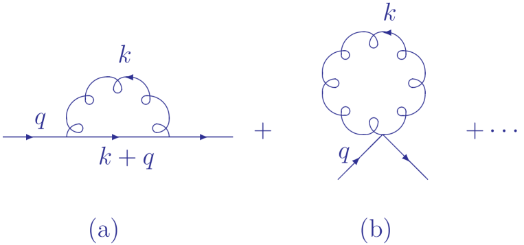
Figure 1: Graviton loop contributions to the scalar propagator. $q$ is the 4-momentum of the scalar.

we have shown in Refs. [9, 10, 11, 12, 13, 14, 15, 16, 17, 18] that the large virtual IR effects in the respective loop integrals for the scalar propagator in quantum general relativity can be resummed to the exact result

$$\begin{split}i\Delta^{\prime}_{F}(k)&=\frac{i}{k^{2}-m^{2}-\Sigma_{s}(k)+i\epsilon}\cr&=\frac{ie^{B^{\prime\prime}_{g}(k)}}{k^{2}-m^{2}-\Sigma^{\prime}_{s}+i\epsilon}\cr&\equiv i\Delta^{\prime}_{F}(k)|_{\text{resummed}}\end{split}$$ (7)

for   ($\Delta=k^{2}-m^{2}$)

$$\begin{split}B^{\prime\prime}_{g}(k)&=-2i\kappa^{2}k^{4}\frac{\int d^{4}\ell}{16\pi^{4}}\frac{1}{\ell^{2}-\lambda^{2}+i\epsilon}\\ &\qquad\frac{1}{(\ell^{2}+2\ell k+\Delta+i\epsilon)^{2}}\\ &=\frac{\kappa^{2}|k^{2}|}{8\pi^{2}}\ln\left(\frac{m^{2}}{m^{2}+|k^{2}|}\right),\end{split}$$ (8)

where the latter form holds for the UV(deep Euclidean) regime, so that (7) falls faster than any power of $|k^{2}|$ – by Wick rotation, the identification $-|k^{2}|\equiv k^{2}$ in the deep Euclidean regime gives immediate analytic continuation to the result in the last line of (8) when the usual $-i\epsilon,\;\epsilon\downarrow 0,$ is appended to $m^{2}$. An analogous result [9] holds for m=0; we show this in our Appendix 1 for completeness. Here, $-i\Sigma_{s}(k)$ is the 1PI scalar self-energy function so that $i\Delta^{\prime}_{F}(k)$ is the exact scalar propagator. As $\Sigma^{\prime}_{s}$ starts in ${\cal O}(\kappa^{2})$, we may drop it in calculating one-loop effects. It follows that, when the respective analogs of (7) are used for the elementary particles, one-loop corrections are finite. It can be shown actually that the use of our resummed propagators renders all quantum gravity loops UV finite [9, 10, 11, 12, 13, 14, 15, 16, 17, 18]. We have called this representation of the quantum theory of general relativity resummed quantum gravity (RQG).

We stress that (7) is not limited to the regime where $k^{2}\cong m^{2}$ but is an identity that holds for all $k^{2}$. This is readily shown as follows. If we invert both sides of (7) we get

$$\Delta_{F}^{-1}(k)-\Sigma_{s}(k)=(\Delta_{F}^{-1}(k)-\Sigma^{\prime}_{s}(k))e^{-B^{\prime\prime}_{g}(k)}$$ (9)

where the free inverse propagator is $\Delta_{F}^{-1}(k)=\Delta(k)+i\epsilon$. We introduce here the loop expansions

$$\Sigma_{s}(k)=\sum_{n=1}^{\infty}\Sigma_{s,n}(k),$$ (10)

$$\Sigma^{\prime}_{s}(k)=\sum_{n=1}^{\infty}\Sigma^{\prime}_{s,n}(k)$$ (11)

and we get, from elementary algebra, the exact relation

$$-\Sigma_{s,n}(k)=-\sum_{j=0}^{n}\Sigma^{\prime}_{s,j}(k)\left(-B^{\prime\prime}_{g}(k)\right)^{n-j}/(n-j)!$$ (12)

where we define for convenience $-\Sigma_{s,0}(k)=-\Sigma^{\prime}_{s,0}(k)=\Delta_{F}^{-1}(k)$ and ${\cal A}_{s,n}$ is the n-loop contribution to ${\cal A}_{s}$. This proves that every Feynman diagram contribution to $\Sigma_{s}(k)$ corresponds to a unique contribution to $\Sigma^{\prime}_{s}(k)$ to all orders in $\kappa^{2}/(4\pi)$ for all values of $k^{2}$. QED.

The key question is whether the terms which we have extracted from the Feynman series in (12) were actually in that series. When we take the limit that $k^{2}\rightarrow m^{2}$, the result is known to be valid from the discussion in Ref. [36] where the same result for the respective exponentiating virtual infrared divergence in (8) is obtained. Indeed, one generally has to introduce a regulator for the IR divergence and one shows that the terms which diverge as the regulator vanishes exponentiate in the factor $B^{\prime\prime}_{g}(k)$. When $k^{2}\neq m^{2}$, the IR divergence is regulated by $\Delta(k)$, so that we can use $\Delta(k)$ as our IR regulator. We can then isolate that part of the amplitude which diverges when $\Delta(k)\rightarrow 0$ when the UV divergences are themselves regulated, by n-dimensional methods [37] for example, so that they remain finite in this limit. At this point we stress the following: when we impose a gauge invariant regulator for the UV regime, to any finite order in the loop expansion, all UV divergences are regulated to finite results. If we then resum the IR dominant terms in this the UV-regulated theory, that resummation is valid independent of whether or not the theory is UV renormalizable, as the theory is finite order by order in the loop expansion in the UV when the UV regulator is imposed independent of whether or not it is renormalizable. The latter issue arises only if we remove the UV regulator. What we show now is that, after the IR resummation, the UV regulator can be removed and the UV regime remains finite order by order in the loop expansion after the IR resummation.

We call attention as well to the close analogy between our use of IR resummation in the presence of n-dimensional UV regularization to study the UV limit of quantum gravity with the use of exact Wilsonian coarse graining in Refs. [2, 3, 4, 5, 6, 7] to arrive at an effective average action for any given scale $k$ which has both an IR cut-off for momentum scales much smaller than $k$ and a UV cut-off for momentum scales much larger than $k$ so that the resulting field-space renormalization group equation is well-defined even for a non-renormalizable theory like quantum gravity. In both cases the UV limit can be studied by taking the UV limit of the resulting non-perturbative solution and in both cases the same result obtains: a non-Gaussian UV fixed point is found, as we present below.

To show that (7) holds with $B^{\prime\prime}_{g}(k)$ given by the expression in (8), we proceed as follows. We represent the respective $m$-loop contribution as defined above to the proper self-energy contribution to the inverse propagator as

$$i\Sigma_{s,m}(p)=\frac{1}{m!}\int\cdots\int\prod_{i=1}^{m}\frac{d^{n}k_{i}}{k_{i}^{2}-\lambda^{2}+i\epsilon}\rho_{m}(k_{1},\cdots,k_{m})$$ (13)

where $n$ is the analytically continued dimension of space-time to regulate UV divergences and the function $\rho_{m}$ is symmetric under the interchange of any two of the m virtual graviton n-momenta that are exchanged in (13), by the Bose symmetry obeyed by the spin 2 gravitons and the symmetry of the respective multiple integration volume. Here is the point in the discussion where the power of exact rearrangement techniques such as those in Ref. [20, 21] enters. For the case $m=1$, let $S^{\prime\prime}_{g}(k)\rho_{0}$ represent the leading contribution in the the limit $k\rightarrow 0$ to $\rho_{1}$. We have

$$\rho_{1}(k)=S^{\prime\prime}_{g}(k)\rho_{0}+\beta_{1}(k)$$ (14)

where this equation is exact and serves to define $\beta_{1}$ if we specify $S^{\prime\prime}_{g}(k)$, the soft graviton emission factor, and recall that

$$\rho_{0}=i\Sigma_{s,0}(p)=-i\Delta_{F}(p)^{-1}.$$ (15)

This can be determined from the Feynman rules for the Feynman [32, 33, 9] formulation of the scalar-graviton system in (6) or one can also use the off-shell extension of the formulas in Ref. [36]. We get [9]

$$\begin{split}S^{\prime\prime}_{g}(p,p,k)&=\frac{1}{(2\pi)^{4}}\frac{i\frac{1}{2}(\eta^{\mu\nu}\eta^{\bar{\mu}\bar{\nu}}+\eta^{\mu\bar{\nu}}\eta^{\bar{\mu}\nu}-\eta^{\mu\bar{\mu}}\eta^{\nu\bar{\nu}})(-i\kappa p_{\bar{\mu}})(2ip_{\mu})(-i\kappa{p^{\prime}}_{\bar{\nu}})(2i{p^{\prime}}_{\nu})}{(k^{2}-2kp+\Delta+i\epsilon)(k^{2}-2kp^{\prime}+\Delta^{\prime}+i\epsilon)}{\Big{|}}_{p=p^{\prime}}\\ &=\frac{2i\kappa^{2}p^{4}}{16\pi^{4}}\frac{1}{(k^{2}-2kp+\Delta+i\epsilon)^{2}}\end{split}$$ (16)

where $\Delta^{\prime}={p^{\prime}}^{2}-m^{2}$. To see this, from Fig. 1, note that the Feynman rules [32, 33, 9] give us the following result

$$\begin{split}i\Sigma_{s,1}(p)&=\Big{\{}-\frac{\int d^{n}k}{(2\pi)^{4}}iv_{3}(p,p-k)_{\mu\bar{\mu}}\frac{i}{(p-k)^{2}-m^{2}+i\epsilon}iv_{3}(p-k,p^{\prime})_{\nu\bar{\nu}}\\ &\qquad\qquad\frac{i\frac{1}{2}(\eta^{\mu\nu}\eta^{\bar{\mu}\bar{\nu}}+\eta^{\mu\bar{\nu}}\eta^{\bar{\mu}\nu}-\eta^{\mu\bar{\mu}}\eta^{\nu\bar{\nu}})}{k^{2}-\lambda^{2}+i\epsilon}\\ &\qquad-\frac{\int d^{n}k}{2(2\pi)^{4}}iv_{4}(p,p^{\prime})_{\mu\bar{\mu};\nu\bar{\nu}}\frac{i\frac{1}{2}(\eta^{\mu\nu}\eta^{\bar{\mu}\bar{\nu}}+\eta^{\mu\bar{\nu}}\eta^{\bar{\mu}\nu}-\eta^{\mu\bar{\mu}}\eta^{\nu\bar{\nu}})}{k^{2}-\lambda^{2}+i\epsilon}\Big{\}}\Big{|}_{p=p^{\prime}},\end{split}$$ (17)

where we have defined from the Feynman rules the respective 3-point($h\varphi\varphi$ and 4-point($hh\varphi\varphi$) vertices

$$\begin{split}iv_{3}(p,p^{\prime})_{\nu\bar{\nu}}&=-i\kappa\left(p_{\nu}{p^{\prime}}_{\bar{\nu}}+p_{\bar{\nu}}{p^{\prime}}_{\nu}-g_{\nu\bar{\nu}}(pp^{\prime}-m^{2})\right)\\ iv_{4}(p,p^{\prime})_{\mu\bar{\mu};\nu\bar{\nu}}&=-4i\kappa^{2}[(pp^{\prime}-m^{2})(\eta_{\mu\bar{\nu}}\eta_{\bar{\mu}\nu}+\eta_{\bar{\mu}\bar{\nu}}\eta_{\mu\nu}-\eta_{\mu\bar{\mu}}\eta_{\nu\bar{\nu}})\\ &\qquad\qquad-(p^{\mu^{\prime}}{p^{\prime}}^{\nu^{\prime}}+p^{\nu^{\prime}}{p^{\prime}}^{\mu^{\prime}})\{\eta_{\mu\mu^{\prime}}(\eta_{\bar{\mu}\nu}\eta_{\nu^{\prime}\bar{\nu}}+\eta_{\bar{\mu}\bar{\nu}}\eta_{\nu^{\prime}\nu}-\eta_{\nu^{\prime}\bar{\mu}}\eta_{\nu\bar{\nu}})\\ &\qquad\qquad+\eta_{\bar{\mu}\mu^{\prime}}(\eta_{\mu\nu}\eta_{\nu^{\prime}\bar{\nu}}+\eta_{\mu\bar{\nu}}\eta_{\nu^{\prime}\nu}-\eta_{\nu^{\prime}\mu}\eta_{\nu\bar{\nu}})\}]\end{split}$$ (18)

using the standard conventions so that p is incoming and p’ is outgoing for the scalar particle momenta at the respective vertices. In this way, we see that we may isolate the IR dominant part of $i\Sigma_{1}(p)$ by the separation

$$\begin{split}\frac{1}{k^{2}-2kp+\Delta+i\epsilon}&=-\frac{\Delta}{(k^{2}-2kp+\Delta+i\epsilon)^{2}}+\frac{1}{k^{2}-2kp+i\epsilon}\\ &\qquad-\frac{2\Delta^{2}}{(k^{2}-2kp+\Delta+i\epsilon)^{2}(k^{2}-2kp+i\epsilon)}\\ &\qquad-\frac{\Delta^{3}}{(k^{2}-2kp+\Delta+i\epsilon)^{2}(k^{2}-2kp+i\epsilon)^{2}}\\ &\qquad+\sum_{n=2}^{\infty}(-1)^{n}\frac{\Delta^{n}}{(k^{2}-2kp+i\epsilon)^{n+1}}\end{split}$$ (19)

from which we can see that the first term on the RHS gives, upon insertion into (17), the IR-divergent contribution for the coefficient of the lowest order inverse propagator for the on-shell limit $\Delta\rightarrow 0$. The second term does not produce an IR-divergence and the remaining terms vanish faster than $\Delta$ in the on-shell limit so that they do not contribute to the field renormalization factor which we seek to isolate. In this way we get finally

$$\begin{split}i\Sigma_{1}(p)&=\Big{\{}-\frac{\int d^{n}k}{(2\pi)^{4}}(-2i\kappa p_{\mu}p_{\bar{\mu}}+i\delta{v_{3}(p,p-k)_{\mu\bar{\mu}}})(\frac{-i\Delta}{(k^{2}-2kp+\Delta+i\epsilon)^{2}}+i~{}R\Delta_{F}(k,p))\\ &\qquad\qquad(-2i\kappa{p}^{\prime}_{\nu}{p^{\prime}}_{\bar{\nu}}+i\delta{v_{3}(p^{\prime}-k,p^{\prime})_{\nu\bar{\nu}}})\frac{i\frac{1}{2}(\eta^{\mu\nu}\eta^{\bar{\mu}\bar{\nu}}+\eta^{\mu\bar{\nu}}\eta^{\bar{\mu}\nu}-\eta^{\mu\bar{\mu}}\eta^{\nu\bar{\nu}})}{k^{2}-\lambda^{2}+i\epsilon}\\ &\qquad-\frac{\int d^{n}k}{2(2\pi)^{4}}iv_{4}(p,p^{\prime})_{\mu\bar{\mu};\nu\bar{\nu}}\frac{i\frac{1}{2}(\eta^{\mu\nu}\eta^{\bar{\mu}\bar{\nu}}+\eta^{\mu\bar{\nu}}\eta^{\bar{\mu}\nu}-\eta^{\mu\bar{\mu}}\eta^{\nu\bar{\nu}})}{k^{2}-\lambda^{2}+i\epsilon}\Big{\}}\Big{|}_{p=p^{\prime}}\\ &\qquad=\Big{\{}\frac{\int d^{n}k}{(2\pi)^{4}}[(-i\kappa p_{\bar{\mu}})(2ip_{\mu})\frac{-i\Delta}{(k^{2}-2kp+\Delta+i\epsilon)^{2}}(-i\kappa{p^{\prime}}_{\bar{\nu}})(2i{p^{\prime}}_{\nu})\\ &\qquad\qquad\frac{i\frac{1}{2}(\eta^{\mu\nu}\eta^{\bar{\mu}\bar{\nu}}+\eta^{\mu\bar{\nu}}\eta^{\bar{\mu}\nu}-\eta^{\mu\bar{\mu}}\eta^{\nu\bar{\nu}})}{k^{2}-\lambda^{2}+i\epsilon}+\frac{(2\pi)^{4}\beta_{1}(k)}{k^{2}-\lambda^{2}+i\epsilon}]\Big{\}}\Big{|}_{p=p^{\prime}},\end{split}$$ (20)

which agrees with (14,15,16) with

$$\begin{split}R\Delta_{F}(k,p)&=\frac{1}{k^{2}-2kp+i\epsilon}-\frac{2\Delta^{2}}{(k^{2}-2kp+\Delta+i\epsilon)^{2}(k^{2}-2kp+i\epsilon)}\\ &\qquad-\frac{\Delta^{3}}{(k^{2}-2kp+\Delta+i\epsilon)^{2}(k^{2}-2kp+i\epsilon)^{2}}\\ &\qquad+\sum_{n=2}^{\infty}(-1)^{n}\frac{\Delta^{n}}{(k^{2}-2kp+i\epsilon)^{n+1}},\\ i\delta{v_{3}(p,p-k)_{\mu\bar{\mu}}}&=iv_{3}(p,p-k)_{\mu\bar{\mu}}-\{-2i\kappa p_{\mu}p_{\bar{\mu}}\},\\ \beta_{1}(k)&=\Big{\{}-\frac{1}{(2\pi)^{4}}(-2i\kappa p_{\mu}p_{\bar{\mu}}+i\delta{v_{3}(p,p-k)_{\mu\bar{\mu}}})[\frac{-i\Delta}{(k^{2}-2kp+\Delta+i\epsilon)^{2}}\\ &\qquad\qquad+i~{}R\Delta_{F}(k,p)](i\delta{v_{3}(p^{\prime}-k,p^{\prime})_{\nu\bar{\nu}}})\{i\frac{1}{2}(\eta^{\mu\nu}\eta^{\bar{\mu}\bar{\nu}}+\eta^{\mu\bar{\nu}}\eta^{\bar{\mu}\nu}-\eta^{\mu\bar{\mu}}\eta^{\nu\bar{\nu}})\}\\ &\qquad\qquad-\frac{1}{(2\pi)^{4}}(-2i\kappa p_{\mu}p_{\bar{\mu}}+i\delta{v_{3}(p,p-k)_{\mu\bar{\mu}}})(i~{}R\Delta_{F}(k,p))\\ &\qquad\qquad(-2i\kappa{p}^{\prime}_{\nu}{p^{\prime}}_{\bar{\nu}})\{i\frac{1}{2}(\eta^{\mu\nu}\eta^{\bar{\mu}\bar{\nu}}+\eta^{\mu\bar{\nu}}\eta^{\bar{\mu}\nu}-\eta^{\mu\bar{\mu}}\eta^{\nu\bar{\nu}})\}\\ &\qquad\qquad-\frac{1}{(2\pi)^{4}}(i\delta{v_{3}(p,p-k)_{\mu\bar{\mu}}})(\frac{-i\Delta}{(k^{2}-2kp+\Delta+i\epsilon)^{2}})\\ &\qquad\qquad(-2i\kappa{p}^{\prime}_{\nu}{p^{\prime}}_{\bar{\nu}})\{i\frac{1}{2}(\eta^{\mu\nu}\eta^{\bar{\mu}\bar{\nu}}+\eta^{\mu\bar{\nu}}\eta^{\bar{\mu}\nu}-\eta^{\mu\bar{\mu}}\eta^{\nu\bar{\nu}})\}\\ &\qquad\qquad-\frac{1}{2(2\pi)^{4}}iv_{4}(p,p^{\prime})_{\mu\bar{\mu};\nu\bar{\nu}}\{i\frac{1}{2}(\eta^{\mu\nu}\eta^{\bar{\mu}\bar{\nu}}+\eta^{\mu\bar{\nu}}\eta^{\bar{\mu}\nu}-\eta^{\mu\bar{\mu}}\eta^{\nu\bar{\nu}})\}\Big{\}}\Big{|}_{p=p^{\prime}}.\end{split}$$ (21)

One can see that the result in (16) differs from the corresponding result in QED in Eq.(5.13) of Ref. [20] by the replacement of the electron charges $e$ by the gravity charges $\kappa p_{\bar{\mu}},~{}\kappa{p^{\prime}}_{\bar{\nu}}$ with the corresponding replacement of the photon propagator numerator $-i\eta_{\mu\nu}$ by the graviton propagator numerator $i\frac{1}{2}(\eta^{\mu\nu}\eta^{\bar{\mu}\bar{\nu}}+\eta^{\mu\bar{\nu}}\eta^{\bar{\mu}\nu}-\eta^{\mu\bar{\mu}}\eta^{\nu\bar{\nu}})$. That the squared modulus of these gravity charges grows quadratically in the deep Euclidean regime is what makes their effect therein in the quantum theory of general relativity fundamentally different from the effect of the QED charges in the deep Euclidean regime of QED, where the latter charges are constants order-by-order in perturbation theory.

Indeed, proceeding recursively, we write

$$\rho_{m}(k_{1},\cdots,k_{m})=S^{\prime\prime}_{g}(k_{m})\rho_{m-1}(k_{1},\cdots,k_{m-1})+\beta^{(1)}_{m}(k_{1},\cdots,k_{m-1};k_{m})$$ (22)

where here the notation indicates that the residual $\beta^{(1)}_{m}$ does not contain the leading infrared contribution for $k_{m}$ that is given by the first term on the RHS of (22). We iterate (22) to get

$$\begin{split}\rho_{m}(k_{1},\cdots,k_{m})&=S^{\prime\prime}_{g}(k_{m})S^{\prime\prime}_{g}(k_{m-1})\rho_{m-2}(k_{1},\cdots,k_{m-2})\\ &+S^{\prime\prime}_{g}(k_{m})\beta^{(1)}_{m-1}(k_{1},\cdots,k_{m-2};k_{m-1})\\ &+S^{\prime\prime}_{g}(k_{m-1})\beta^{(1)}_{m-1}(k_{1},\cdots,k_{m-2};k_{m})\\ &+\{-S^{\prime\prime}_{g}(k_{m-1})\beta^{(1)}_{m-1}(k_{1},\cdots,k_{m-2};k_{m})+\beta^{(1)}_{m}(k_{1},\cdots,k_{m-1};k_{m})\}\end{split}$$ (23)

The symmetry of $\rho_{m}$ implies that the quantity in curly brackets is also symmetric in the interchange of $k_{m-1}$ and $k_{m}$. We indicate this explicitly with the notation

$$\{-S^{\prime\prime}_{g}(k_{m-1})\beta^{(1)}_{m-1}(k_{1},\cdots,k_{m-2};k_{m})+\beta^{(1)}_{m}(k_{1},\cdots,k_{m-1};k_{m})\}=\beta^{(2)}_{m}(k_{1},\cdots,k_{m-2};k_{m-1},k_{m}).$$ (24)

Repeated application of (22) and use of the symmetry of $\rho_{m}$ leads us finally to the exact result

$$\begin{split}\rho_{m}(k_{1},\cdots,k_{m})&=S^{\prime\prime}_{g}(k_{1})\cdots S^{\prime\prime}_{g}(k_{m})\beta_{0}\\ &+\sum_{i=1}^{m}S^{\prime\prime}_{g}(k_{1})\cdots S^{\prime\prime}_{g}(k_{i-1})S^{\prime\prime}_{g}(k_{i+1})\cdots S^{\prime\prime}_{g}(k_{m})\beta_{1}(k_{i})\\ &+\cdots+\sum_{i=1}^{m}S^{\prime\prime}_{g}(k_{i})\beta_{m-1}(k_{1},\cdots,k_{i-1},k_{i+1},\cdots,k_{m})+\beta_{m}(k_{1},\cdots,k_{m})\end{split}$$ (25)

where the case m=1 has already been considered in (14) with $\rho_{0}\equiv\beta_{0}$. Here, we defined as well $\beta^{(i)}_{i}\equiv\beta_{i}$.

We can use the symmetry of the residuals $\beta_{i}$ to re-write $\rho_{m}$ as

$$\rho_{m}(k_{1},\cdots,k_{m})=\sum_{perm}\sum_{r=0}^{m}\frac{1}{r!(m-r)!}\prod_{i=1}^{r}S^{\prime\prime}_{g}(k_{i})\beta_{m-r}(k_{r+1},\cdots,k_{m})$$ (26)

so that we finally obtain, upon substitution into (13),

$$i\Sigma_{s,m}(p)=\sum_{r=0}^{m}\frac{1}{r!(m-r)!}\left(\int\frac{d^{n}k~{}S^{\prime\prime}_{g}(k)}{k^{2}-\lambda^{2}+i\epsilon}\right)^{r}\int\prod_{i=1}^{m-r}\frac{d^{n}k_{i}}{{k_{i}}^{2}-\lambda^{2}+i\epsilon}\beta_{m-r}(k_{1},\cdots,k_{m-r}).$$ (27)

With the definition

$$-B^{\prime\prime}_{g}(p)=\int\frac{d^{n}k~{}S^{\prime\prime}_{g}(k)}{k^{2}-\lambda^{2}+i\epsilon}$$ (28)

and the identification

$$i\Sigma^{\prime}_{s,r}(p)=\frac{1}{r!}\int\prod_{i=1}^{r}\frac{d^{n}k_{i}}{k_{i}^{2}-\lambda^{2}+i\epsilon}\beta_{r}(k_{1},\cdots,k_{r})$$ (29)

we introduce the result (27) into (9) via (10) to get

$$\begin{split}-i\left(\Delta_{F}(p)^{-1}-\Sigma_{s}(p)\right)&=i\sum_{m=0}^{\infty}\sum_{r=0}^{m}\Sigma^{\prime}_{s,m-r}(p)\frac{(-B^{\prime\prime}_{g}(p))^{r}}{r!}\\ &=ie^{-B^{\prime\prime}_{g}(p)}\sum_{\ell=0}^{\infty}\Sigma^{\prime}_{s,\ell}(p)\\ &=-ie^{-B^{\prime\prime}_{g}(p)}\left(\Delta_{F}(p)^{-1}-\sum_{\ell=1}^{\infty}\Sigma^{\prime}_{s,\ell}(p)\right).\end{split}$$ (30)

In this way, our resummed exact result for the complete scalar propagator in quantum general relativity is seen to be [9, 11, 12, 13]

$$\begin{split}i\Delta^{\prime}_{F}(p)&=\frac{ie^{B^{\prime\prime}_{g}(p)}}{(p^{2}-m^{2}-\Sigma^{\prime}_{s}(p)+i\epsilon)}\cr&\equiv i\Delta^{\prime}_{F}(p)|_{\text{resummed}}\equiv i\Delta^{\prime}_{F}(p)|_{\text{rsm}}\end{split}$$ (31)

where

$$\Sigma^{\prime}_{s}(p)\equiv\sum_{\ell=1}^{\infty}\Sigma^{\prime}_{s,\ell}(p).$$ (32)

We have introduced the shorthand “rsm” for “resummed” in the last line of (31) for later convenience.

This result (32) becomes identical to (7) when we take the limit $n\rightarrow 4$ in it. In taking this limit, we note that $B^{\prime\prime}_{g}(k)$ is UV finite so that the limit exists without further ado. As the IR limit of the coupling of the graviton to a particle is well-known [36] to independent of its spin, the entirely analogous result to (32) holds for the propagators of all particles [9, 11, 12, 13] with corresponding exponent $B^{\prime\prime}_{g}(k)$ and the attendant IR-improved proper self-energy function. We note that in $\Sigma^{\prime}_{s}(p)$ the limit $n\rightarrow 4$ can be taken if we represent it by its IR-improved propagator expansion in which, to any finite order in the loop expansion, the usual free Feynman propagator is replaced by its resummed version with the attendant IR-improved proper self-energy function, $\Sigma^{\prime}_{s}(p)$ or its graviton analog, set to zero on at least one internal line (per loop): for the scalar case this reads

$$i\Delta_{F}(p)|_{\text{resummed}}=\frac{ie^{B^{\prime\prime}_{g}(p)}}{(p^{2}-m^{2}+i\epsilon)}.$$ (33)

with a corresponding result for the graviton case. Standard resummation algebra then can be used to remove any double counting effects to any finite order in the loop expansion, as $B^{\prime\prime}_{g}(k)$ is a UV finite one-loop effect. Let us now see how one proves this last remark.

To this end, let $\Gamma^{\ell,m}(k_{1},\ldots,k_{\ell};k^{\prime}_{1},\ldots,k^{\prime}_{m})$ be the 1PI $\ell$-graviton, m-scalar proper vertex function, where we suppress all Lorentz indices without loss of content. We follow Ref. [38] and write $\Gamma^{\ell,m}(k_{1},\ldots,k_{\ell};k^{\prime}_{1},\ldots,k^{\prime}_{m})$ in terms of its skeleton expansion in which, to any finite order in the respective loop expansion, each graph ${\cal G}$ is mapped into a unique skeleton ${\cal S}$ in which all corrections to propagators and interaction vertices are removed. We then have the identification

$$\Gamma^{\ell,m}(k_{1},\ldots,k_{\ell};k^{\prime}_{1},\ldots,k^{\prime}_{m})=\sum_{\text{skeletons}\;{\cal S}}\Gamma^{{\cal S},\ell,m}(k_{1},\ldots,k_{\ell};k^{\prime}_{1},\ldots,k^{\prime}_{m};\Delta^{\prime}_{F},D^{\prime}_{F},\{\Gamma_{j}\},\kappa)$$ (34)

following the recipe in Ref. [38] so that here one uses the complete propagators, $\Delta^{\prime}_{F},D^{\prime}_{F}$, for the scalar and the graviton on the lines of the skeleton and one uses the complete interaction vertex foundations $\{\Gamma_{j}\}$ at each respective vertex in the skeleton to produce the exact, complete result for $\Gamma^{\ell,m}(k_{1},\ldots,k_{\ell};k^{\prime}_{1},\ldots,k^{\prime}_{m})$. In this representation, it is immediate how to obtain the attendant $N$-th loop result accurate up to and including the $N$-th loop for $\Gamma^{\ell,m}(k_{1},\ldots,k_{\ell};k^{\prime}_{1},\ldots,k^{\prime}_{m})$: one expands the propagators and complete interaction vertices to the appropriate order, $\leq N$ and retains all terms with $\leq N$ loops in the sum on the RHS of (34). In the case of the exact scalar propagator, for example, we expand it as usual in each term in (34),

$$i\Delta^{\prime}_{F}(p)=i\Delta_{F}(p)+i\Delta_{F}(p)(-i\Sigma_{s}(p))i\Delta_{F}(p)+\cdots,$$ (35)

and we stop at the term with $N$-factors of $(-i\Sigma_{s}(k))$ each one of which we evaluate only to one loop order in this last term, with the attendant higher loop evaluations in the terms with less than $N$ factors by the standard methodology. Inserting this result into (34) with the analogous ones for the graviton propagator and the interaction vertices we isolate the result accurate up to and including the $N$-th loop by dropping all contributions that involve more than $N$-loops. This is the standard Feynman diagrammatic practice. Since we have the n-dimensional regulation of the UV divergences, the result we obtain this way is UV finite.

To improve it we substitute the resummed representation for the propagators, which we denote as we have above so that we have

$$\Gamma^{\ell,m}(k_{1},\ldots,k_{\ell};k^{\prime}_{1},\ldots,k^{\prime}_{m})=\sum_{\text{skeletons}\;{\cal S}}\Gamma^{{\cal S},\ell,m}(k_{1},\ldots,k_{\ell};k^{\prime}_{1},\ldots,k^{\prime}_{m};{\Delta^{\prime}_{F}}|_{\text{rsm}},{D^{\prime}_{F}}|_{\text{rsm}},\{\Gamma_{j}\},\kappa)$$ (36)

To obtain the IR-improved result correct up to an including the $N$-th IR-improved loop, we repeat the same steps as we did for the un-improved case: for example, we expand the scalar propagator as

$$\begin{split}i\Delta^{\prime}_{F}(p)&=\frac{ie^{B^{\prime\prime}_{g}(p)}}{(p^{2}-m^{2}-\Sigma^{\prime}_{s}(p)+i\epsilon)}\cr&=ie^{B^{\prime\prime}_{g}(p)}\left(\Delta_{F}(p)+\Delta_{F}(p)(-i\Sigma^{\prime}_{s}(p))i\Delta_{F}(p)+\cdots\right)\end{split}$$ (37)

where we now stop the expansion at the term with $N$-factors of $(-i\Sigma^{\prime}_{s}(p))$ in which each factor is only computed to one-loop order. We then introduce this IR-improved $N$-loop result for the scalar propagator and the analogous results for the graviton propagator and the interaction vertices accurate as well to $N$ loops in the IR-improved loops into the the RHS of (36) and drop all terms with more than $N$ IR-improved loops. The result is now UV finite because the exponential factor in the respective propagators render the integration in deep UV finite for any finite order in the interaction strength $\kappa$ because these exponential factors fall faster than any of the finite powers of the loop momenta that occur at finite orders in $\kappa$ as given by the Feynman rules that follow from Refs. [32, 33] for (6).

Finally, we observe that (12) can be inverted to give as well the identity

$$-\Sigma^{\prime}_{s,n}(k)=-\sum_{j=0}^{n}\Sigma_{s,j}(k)\left(B^{\prime\prime}_{g}(k)\right)^{n-j}/(n-j)!$$ (38)

This allows us to employ the same result (36) in calculating the IR-improved self-energy so that it too is now UV finite with our IR-improved resummation prescription. It follows that, to any finite order in the IR-improved loop expansion, all $\Gamma^{\ell,m}(k_{1},\ldots,k_{\ell};k^{\prime}_{1},\ldots,k^{\prime}_{m})$ are UV finite. QED

As we have indicated above [9] and as Weinberg has shown in Ref. [36], the IR limit of the coupling of the graviton to a particle is independent of its spin, so that we get the same exponential behavior in the resummed propagator for all particles in the Standard Model. Indeed, when we use our resummed propagator results, as extended to all the particles in the SM Lagrangian and to the graviton itself, working now with the complete theory

$${\cal L}(x)=\frac{1}{2\kappa^{2}}\sqrt{-g}\left(R-2\Lambda\right)+\sqrt{-g}L^{\cal G}_{SM}(x)$$ (39)

where $L^{\cal G}_{SM}(x)$ is SM Lagrangian written in diffeomorphism invariant form as explained in Refs. [9, 11], we show in the Refs. [9, 10, 11, 12, 13, 14, 15, 16, 17, 18] that the denominator for the propagation of transverse-traceless modes of the graviton becomes ($M_{Pl}$ is the Planck mass)

$$q^{2}+\Sigma^{T}(q^{2})+i\epsilon\cong q^{2}-q^{4}\frac{c_{2,eff}}{360\pi M_{Pl}^{2}},$$ (40)

where we have defined

$$\begin{split}c_{2,eff}&=\sum_{\text{SM particles j}}n_{j}I_{2}(\lambda_{c}(j))\\ &\cong 2.56\times 10^{4}\end{split}$$ (41)

with $I_{2}$ defined [9, 10, 11, 12, 13, 14, 15, 16, 17, 18] by

$$I_{2}(\lambda_{c})=\int^{\infty}_{0}dxx^{3}(1+x)^{-4-\lambda_{c}x}$$ (42)

and with $\lambda_{c}(j)=\frac{2m_{j}^{2}}{\pi M_{Pl}^{2}}$ and [9, 10, 11, 12, 13, 14, 15, 16, 17, 18] $n_{j}$ equal to the number of effective degrees of particle $j$. For completeness, we repeat the derivation of (40) in our Appendix 2, using results from Appendix 3. In arriving at the numerical value in (41), we take the SM masses as follows: for the now presumed three massive neutrinos [39, 40], we estimate a mass at $\sim 3$ eV; for the remaining members of the known three generations of Dirac fermions $\{e,\mu,\tau,u,d,s,c,b,t\}$, we use [41, 42, 43] $m_{e}\cong 0.51$ MeV, $m_{\mu}\cong 0.106$ GeV, $m_{\tau}\cong 1.78$ GeV, $m_{u}\cong 5.1$ MeV, $m_{d}\cong 8.9$ MeV, $m_{s}\cong 0.17$ GeV, $m_{c}\cong 1.3$ GeV, $m_{b}\cong 4.5$ GeV and $m_{t}\cong 174$ GeV and for the massive vector bosons $W^{\pm},~{}Z$ we use the masses $M_{W}\cong 80.4$ GeV, $M_{Z}\cong 91.19$ GeV, respectively. We set the Higgs mass at $m_{H}\cong 126$GeV, in view of the limit from LEP2 [44, 45] and recent observations from ATLAS and CMS [46]. We note that (see the Appendix 1) when the rest mass of particle $j$ is zero, such as it is for the photon and the gluon, the value of $m_{j}$ turns-out to be $\sqrt{2}$ times the gravitational infrared cut-off mass [29, 30], which is $m_{g}\cong 3.1\times 10^{-33}$eV. We further note that, from the exact one-loop analysis of Ref.[47], it also follows (see Appendix 2) that the value of $n_{j}$ for the graviton and its attendant ghost is $42$. For $\lambda_{c}\rightarrow 0$, we have found the approximate representation (see Appendix 3)

$$I_{2}(\lambda_{c})\cong\ln\frac{1}{\lambda_{c}}-\ln\ln\frac{1}{\lambda_{c}}-\frac{\ln\ln\frac{1}{\lambda_{c}}}{\ln\frac{1}{\lambda_{c}}-\ln\ln\frac{1}{\lambda_{c}}}-\frac{11}{6}.$$ (43)

These results allow us to identify (we use $G_{N}$ for $G_{N}(0)$)

$$G_{N}(k)=G_{N}/(1+\frac{c_{2,eff}k^{2}}{360\pi M_{Pl}^{2}})$$ (44)

and to compute the UV limit $g_{*}$ as

$$g_{*}=\lim_{k^{2}\rightarrow\infty}k^{2}G_{N}(k^{2})=\frac{360\pi}{c_{2,eff}}\cong 0.0442.$$ (45)

We stress that this result has no threshold/cut-off effects in it. It is a pure property of the known world.

Turning now to the prediction for $\lambda_{*}$, we use the Euler-Lagrange equations to get Einstein’s equation as

$$G_{\mu\nu}+\Lambda g_{\mu\nu}=-\kappa^{2}T_{\mu\nu}$$ (46)

in a standard notation where $G_{\mu\nu}=R_{\mu\nu}-\frac{1}{2}Rg_{\mu\nu}$, $R_{\mu\nu}$ is the contracted Riemann tensor, and $T_{\mu\nu}$ is the energy-momentum tensor. Working then with the representation $g_{\mu\nu}=\eta_{\mu\nu}+2\kappa h_{\mu\nu}$ for the flat Minkowski metric $\eta_{\mu\nu}=\text{diag}(1,-1,-1,-1)$ we see that to isolate $\Lambda$ in Einstein’s equation (46) we may evaluate its VEV(vacuum expectation value of both sides). For any bosonic quantum field $\varphi$ we use the point-splitting definition (here, :  : denotes normal ordering as usual)

$$\begin{split}\varphi(0)\varphi(0)&=\lim_{\epsilon\rightarrow 0}\varphi(\epsilon)\varphi(0)\cr&=\lim_{\epsilon\rightarrow 0}T(\varphi(\epsilon)\varphi(0))\cr&=\lim_{\epsilon\rightarrow 0}\{:(\varphi(\epsilon)\varphi(0)):+<0|T(\varphi(\epsilon)\varphi(0))|0>\}\cr\end{split}$$ (47)

where the limit $\epsilon\equiv(\epsilon,\vec{0})\rightarrow(0,0,0,0)\equiv 0$ is taken from a time-like direction respectively. Thus, a scalar makes the contribution to $\Lambda$ given by

$$\begin{split}\Lambda_{s}&=-8\pi G_{N}\frac{\int d^{4}k}{2(2\pi)^{4}}\frac{(2k_{0}^{2})e^{-\lambda_{c}(k^{2}/(2m^{2}))\ln(k^{2}/m^{2}+1)}}{k^{2}+m^{2}}\cr&\cong-8\pi G_{N}[\frac{1}{G_{N}^{2}64\rho^{2}}],\cr\end{split}$$ (48)

where $\rho=\ln\frac{2}{\lambda_{c}}$ and we have used the calculus of Refs. [9, 10, 11, 12, 13, 14, 15, 16, 17, 18] as recapitulated here in Appendices 2,3. The standard equal-time (anti-)commutation relations algebra realizations then show that a Dirac fermion contributes $-4$ times $\Lambda_{s}$ to $\Lambda$. The deep UV limit of $\Lambda$ then becomes, allowing $G_{N}(k)$ to run as we calculated,

$$\begin{split}\Lambda(k)&\operatornamewithlimits{\longrightarrow}_{k^{2}\rightarrow\infty}k^{2}\lambda_{*},\cr\lambda_{*}&=-\frac{c_{2,eff}}{2880}\sum_{j}(-1)^{F_{j}}n_{j}/\rho_{j}^{2}\cr&\cong 0.0817\end{split}$$ (49)

where $F_{j}$ is the fermion number of $j$, $n_{j}$ is the effective number of degrees of freedom of $j$ and $\rho_{j}=\rho(\lambda_{c}(m_{j}))$. We see again that $\lambda_{*}$ is free of threshold/cut-off effects and is a pure prediction of our known world – $\lambda_{*}$ would vanish in an exactly supersymmetric theory.

For reference, the UV fixed-point calculated here, $(g_{*},\lambda_{*})\cong(0.0442,0.0817)$, can be compared with the estimates in Refs. [24, 25], which give $(g_{*},\lambda_{*})\approx(0.27,0.36)$. In making this comparison, one must keep in mind that the analysis in Refs. [24, 25] did not include the specific SM matter action and that there is definitely cut-off function sensitivity to the results in the latter analyses. What is important is that the qualitative results that $g_{*}$ and $\lambda_{*}$ are both positive and are less than 1 in size are true of our results as well.

For reference, we note that, if we restrict our resummed quantum gravity calculations above for $g_{*},\lambda_{*}$ to the pure gravity theory with no SM matter fields, we get the results

$$g_{*}=.0533,\;\lambda_{*}=-.000189.$$

We see that our results suggest that there are still significant cut-off effects in the results used for $g_{*},\;\lambda_{*}$ in Refs. [24, 25], which already seem to include an effective matter contribution when viewed from our resummed quantum gravity perspective, as an artifact of the obvious gauge and cut-off dependencies of the results. Indeed, from a purely quantum field theoretic point of view, the cut-off action is

$$\Delta_{k}S(h,C,\bar{C};\bar{g})=\frac{1}{2}<h,{\cal R}^{\text{grav}}_{k}h>+<\bar{C},{\cal R}^{\text{gh}}_{k}C>$$ (50)

where $\bar{g}$ is the general background metric, which is the Minkowski space metric $\eta$ here, and $C,\bar{C}$ are the ghost fields and the operators ${\cal R}^{\text{grav}}_{k},\;{\cal R}^{\text{gh}}_{k}$ implement the course graining as they satisfy the limits

$$\begin{split}{\underset{p^{2}/k^{2}\rightarrow\infty}{\text{lim}}}{\cal R}_{k}&=0,\\ {\underset{p^{2}/k^{2}\rightarrow 0}{\text{lim}}}{\cal R}_{k}&\rightarrow\mathfrak{Z}_{k}k^{2},\end{split}$$

for some $\mathfrak{Z}_{k}$ [3]. Here, the inner product is that defined in Ref. [3] in its Eqs.(2.14,2.15,2.19). The result is that the modes with $p\lesssim k$ have a shift of their vacuum energy by the cut-off operator. There is therefore no disagreement in principle between our gauge invariant results and the gauge dependent and cut-off dependent results in Refs. [3]. In other words, the graviton and ghost fields at low scales compared to k have a mass added to them, so that their vacuum energies are shifted by a mass of order k. Evidently, this shows up as a positive contribution to the cosmological constant and explains why the EFRG result for $\lambda_{*}$ has a positive value in the regime of the gauge parameter in Ref. [3] where the UV fixed point is attractive.

4 An Estimate of $\Lambda$

To see that the results here, taken together with those in Refs. [24, 25], allow us to estimate the value of $\Lambda$ today, we take the normal-ordered form of Einstein’s equation

$$:G_{\mu\nu}:+\Lambda:g_{\mu\nu}:=-\kappa^{2}:T_{\mu\nu}:.$$ (51)

The coherent state representation of the thermal density matrix then gives the Einstein equation in the form of thermally averaged quantities with $\Lambda$ given by our result in (LABEL:lambscalar) summed over the degrees of freedom as specified above in lowest order. In Ref. [25], it is argued that the Planck scale cosmology description of inflation needs the transition time between the Planck regime and the classical Friedmann-Robertson-Walker(FRW) regime at $t_{tr}\sim 25t_{Pl}$. (We comment below on the uncertainty of this choice of $t_{tr}$.) We thus introduce

$$\begin{split}\rho_{\Lambda}(t_{tr})&\equiv\frac{\Lambda(t_{tr})}{8\pi G_{N}(t_{tr})}\cr&=\frac{-M_{Pl}^{4}(k_{tr})}{64}\sum_{j}\frac{(-1)^{F}n_{j}}{\rho_{j}^{2}}\end{split}$$ (52)

and use the arguments in Refs. [49] ($t_{eq}$ is the time of matter-radiation equality) to get the first principles estimate, from the method of the operator field,

$$\begin{split}\rho_{\Lambda}(t_{0})&\cong\frac{-M_{Pl}^{4}(1+c_{2,eff}k_{tr}^{2}/(360\pi M_{Pl}^{2}))^{2}}{64}\sum_{j}\frac{(-1)^{F}n_{j}}{\rho_{j}^{2}}\cr&\qquad\quad\times\frac{t_{tr}^{2}}{t_{eq}^{2}}\times(\frac{t_{eq}^{2/3}}{t_{0}^{2/3}})^{3}\cr&\cong\frac{-M_{Pl}^{2}(1.0362)^{2}(-9.194\times 10^{-3})}{64}\frac{(25)^{2}}{t_{0}^{2}}\cr&\cong(2.4\times 10^{-3}eV)^{4}.\end{split}$$ (53)

where we take the age of the universe to be $t_{0}\cong 13.7\times 10^{9}$ yrs. In the latter estimate, the first factor in the second line comes from the period from $t_{tr}$ to $t_{eq}$ which is radiation dominated and the second factor comes from the period from $t_{eq}$ to $t_{0}$ which is matter dominated . This estimate should be compared with the experimental result [30] $\rho_{\Lambda}(t_{0})|_{\text{expt}}\cong((2.37\pm 0.05)\times 10^{-3}eV)^{4}$.

To sum up, in addition to our having put the Planck scale cosmology [24, 25] on a more rigorous basis, we believe our estimate of $\rho_{\Lambda}(t_{0})$ represents some amount of progress in the long effort to understand its observed value in quantum field theory. Evidently, the estimate is not a precision prediction, as hitherto unseen degrees of freedom may exist and they have not been included, for example.

Indeed, we see that our result for the contribution to $\Lambda$ from a particle of rest mass $m$ scales as $1/\ln^{2}(2/\lambda_{c}(m))$ so that for masses $m<<M_{Pl}$ the larger the mass, the larger the contribution in magnitude. We note that the t, b, c, s, d, u, $\tau$, $\mu$, e and the three neutrinos (together) contribute respectively 21.1%, 17.6%, 16.7%, 15.2% , 13.5%, 13.2%, 5.63%, 4.97%, 4.01% and 7.93% of $\Lambda$ whereas the Higgs, W and Z bosons contribute -1.73%, -5.10% and -10.1% of $\Lambda$ respectively. The photon and the gluon, taken together, contribute -2.51% of $\Lambda$, while the graviton contributes -0.277% thereof. Naively, such dependence on particle mass might appear to contradict the Appelquist-Carazzone decoupling theorem [51], by which larger values of $m$ might be expected to be more suppressed. Two comments are in order. First, the decoupling theorem in Ref. [51] was only proved for renormalizable theories whereas the Einstein-Hilbert theory we deal with here is (power-countingly) nonrenormalizable. After we resum the theory, it is UV finite with a characteristic scale of $\sim M_{Pl}$ for the scale beyond which the UV modes are suppressed. Again, this is not the hypothesis of the Appelquist-Carazzone theorem. The key is the scale $M_{Pl}$. In the analyses presented above, we assume that $m/M_{Pl}<<1$ in deriving our results. For a quantity such as the integral on the RHS of the (LABEL:lambscalar) for $\Lambda_{s}$, which diverges like 4-powers of the cut-off without resummation and which has a dependence on $M_{Pl}^{4}$ when we resum the theory, the remaining dependence on the particle mass $m$ arises from the strength of the suppression of the modes beyond the characteristic scale $M_{Pl}$ and this is stronger for the smaller values of $m$ because they are farther away from $M_{Pl}$ which dominates the integral, as we expect from the uncertainty principle. This phenomenon becomes even more transparent if we consider masses $m>>M_{Pl}$, so that we are not subject to effects of finite physical intrinsic scales. For two masses $m_{1},\;m_{2}$ satisfying $m_{i}>>M_{Pl}$, we calculate that the contribution to $\Lambda_{s}$ scales as $m_{i}M_{Pl}$ so that we have the behavior one would expect from summing the zero modes of a field of rest mass $m_{i}$ when the resummation causes the phase space integral to cut-off at a scale $\sim M_{Pl}$ yielding the factor $-8\pi G_{N}(M_{Pl}^{3}m_{i})$ since the vacuum energy density of the field is given by (Here ${\cal H}$ is the usual free field Hamiltonian density.)

$$<0|{\cal H}|0>\sim\int^{M_{Pl}}\frac{d^{3}k}{(2\pi)^{3}}\frac{1}{2}\omega(k)=\int^{M_{Pl}}\frac{d^{3}k}{(2\pi)^{3}}\frac{1}{2}\sqrt{k^{2}+m_{i}^{2}}$$

where $\omega(k)$ is the usual frequency for mode $\vec{k}$ of the field and reduces to $m_{i}$ when $k^{2}<<m_{i}^{2}$. The larger mass makes a larger contribution because its zero modes are larger. This naturally raises the question of what would happen to our estimate if there would be a GUT theory at high scale? We now comment on this.

In the current status of the standard GUT phenomenology, we know that the main viable approaches involve susy GUT’s because the standard non-susy models have trouble to match the value of $\sin^{2}\theta_{W}$ and have the three $SU_{2L}\times U_{1}\times SU(3)^{c}$ couplings [52, 53] meet given their now precise values [30, 54] at the scale $M_{Z}$, the rest mass of the $Z^{0}$ heavy gauge boson in the Glashow-Salam-Weinberg theory[52]. To illustrate how a susy GUT might affect our estimate of $\Lambda$ we use the susy SO(10) GUT model in Ref. [55] for definiteness.

In this model, the break-down of the GUT gauge symmetry to the low energy gauge symmetry occurs with an intermediate stage with gauge group $SU_{2L}\times SU_{2R}\times U_{1}\times SU(3)^{c}$ where the final break-down to the Standard Model [52, 53] gauge group, $SU_{2L}\times U_{1}\times SU(3)^{c}$, occurs at a scale $M_{R}\gtrsim 2TeV$ while the breakdown of global susy occurs at the (EW) scale $M_{S}$ which satisfies $M_{R}>M_{S}$. For our purposes the key observation is that susy multiplets do not contribute to our formula in (52) when susy is not broken – there is exact cancellation between fermions and bosons in a given degenerate susy multiplet. Thus only the the broken susy multiplets can contribute. In the model at hand, these are just the multiplets associated with the known SM particles and the extra Higgs multiplet required by susy in the MSSM [56]. In view of recent LHC results [57], we take for illustration the values $M_{R}\cong 4M_{S}\sim 2.0{\text{TeV}}$ and set the following susy partner values:

$$\begin{split}m_{\tilde{g}}&\cong 1.5(10){\text{TeV}}\\ m_{\tilde{G}}&\cong 1.5{\text{TeV}}\\ m_{\tilde{q}}&\cong 1.0{\text{TeV}}\\ m_{\tilde{\ell}}&\cong 0.5{\text{TeV}}\\ m_{\tilde{\chi}^{0}_{i}}&\cong\begin{cases}&0.4{\text{TeV}},\;i=1\\ &0.5{\text{TeV}},\;i=2,3,4\end{cases}\\ m_{\tilde{\chi}^{\pm}_{i}}&\cong 0.5{\text{TeV}},\;i=1,2\\ m_{S}&=.5{\text{TeV}},\;S=A^{0},\;H^{\pm},\;H_{2},\end{split}$$ (54)

where we use a standard notation for the susy partners of the known quarks($q\leftrightarrow\tilde{q}$), leptons($\ell\leftrightarrow\tilde{\ell}$) and gluons($G\leftrightarrow\tilde{G}$), and the EW gauge and Higgs bosons($\gamma,\;Z^{0},\;W^{\pm},\;H,$
$A^{0},\;H^{\pm},\;H_{2}\leftrightarrow\tilde{\chi}$) with the extra Higgs particles denoted as usual [56] by $A^{0}$(pseudo-scalar), $H^{\pm}$(charged) and $H_{2}$(heavy scalar). $\tilde{g}$ is the gravitino, for which we show two examples of its mass for illustration. These particles then generate the extra contribution

$$\begin{split}\Delta W_{\rho,\text{GUT}}&=\sum_{j\in\{\text{MSSM low energy susy partners}\}}\frac{(-1)^{F}n_{j}}{\rho_{j}^{2}}\\ &\cong 1.13(1.12)\times 10^{-2}\end{split}$$ (55)

to the factor $W_{\rho}\equiv\sum_{j}\frac{(-1)^{F}n_{j}}{\rho_{j}^{2}}$ on the RHS of (52) for the two respective values of $m_{\tilde{g}}$ called out by the parentheses. The corresponding values of $\rho_{\Lambda}$ are $-(1.67\times 10^{-3}\text{eV})^{4}(-(1.65\times 10^{-3}\text{eV})^{4})$, respectively. The sign of these results would appear to put them in conflict with the positive observed value quoted above by many standard deviations, even when we allow for the considerable uncertainty in the various other factors multiplying $W_{\rho}$ in (52), all of which are positive in our framework. This may be alleviated either by adding new particles to the model, approach (A), or by allowing a soft susy breaking mass term for the gravitino that resides near the GUT scale $M_{GUT}$, which is $\sim 4\times 10^{16}GeV$ here [55], approach (B). In approach (A), we double the number of quarks and leptons, but we invert the mass hierarchy between susy partners, so that the new squarks and sleptons are lighter than the new quarks and leptons. This can work as long as as we increase $M_{R},\;M_{S}$ so that we have the new quarks and leptons at $M_{\text{High}}\sim 3.4(3.3)\times 10^{3}\text{TeV}$ while leaving their partners at $M_{\text{Low}}\sim.5{\text{TeV}}$. For approach (B), the mass of the gravitino soft breaking term should be set to $m_{\tilde{g}}\sim 2.3\times 10^{15}{\text{GeV}}$. More generally, our estimate in (53) can be used as a constraint of general susy GUT models and we hope to explore such in more detail elsewhere. This admittedly limited discussion of susy GUT effects highlights what one can expect for the impact on our estimate in (53) from higher mass scale physics.

Moreover, we need to stress that the value of $t_{tr}$ cannot be taken as precise, as we now elaborate. Specifically, we are using for it the theory of Ref. [25]. We can see that the solution to the renormalization group improved Einstein equations in Ref. [25] relates $M_{Pl}\cong\xi H(t_{tr})\cong\alpha/t_{tr}$ where $\alpha=1/(2-2\Omega_{\Lambda}^{*})$ with $\Omega_{\Lambda}^{*}$ equal to the relative vacuum energy in the UV fixed point regime so that $\Omega_{\Lambda}^{*}\in(0,1)$. Here, $H$ is the Hubble parameter as usual and $\xi$ is of order unity and positive. For power law Planck scale inflation, we need $\alpha>1$, or $\Omega_{\Lambda}^{*}>1/2$. The authors in Ref. [25] take as ’generic’ $\Omega_{\Lambda}^{*}=0.98$ which leads to $\alpha=25$ and in the solution to their renormalization group improved Einstein equations to the $t_{tr}=\alpha t_{Pl}=25t_{Pl}$ that we have used here. Taking the difference between $\Omega_{\Lambda}^{*}$ and $1$ an order of magnitude smaller would amount to fine tuning, so it is probably unreasonable. In addition, in order to match smoothly onto the FRW classical solution, $t_{tr}$ cannot be too close to $t_{Pl}$, where the classical solution surely fails. Thus, we need $\alpha$ significantly larger than 1. In other words, what the authors in Ref. [25] have taken really does seem to be ’generic’, as they put it. We feel $t_{tr}$ could be smaller by a factor $\sim 3$ and could be larger by a similar factor and still be ’generic’. Even this error estimate alone would mean that our final result for $\rho_{\Lambda}$ is at least uncertain at the factor of $10$ level in the Bonanno and Reuter model. This should be taken in addition to the uncertainty associated with the relation between the momentum scale $k$ and the cosmological time $t$ as we have indicated above for Ref. [25], where the estimates here realize this via Eqs.(2.2) and (5.1) in Ref. [25], $k(t)=\xi H(t)\cong\alpha/t$. Given that we are switching from the Planck regime to the FRW regime, there is uncertainty in $t_{tr}$ from both pieces of this last relation. Realistically, especially given the non-rigorousness of any argument based on fine tuning, we actually do not know the precise value of $t_{tr}$ at this point to better than a couple of orders of magnitude which translate to a conservative uncertainty at the level of $10^{4}$ on our estimate of $\rho_{\Lambda}$. We caution the reader to keep this in mind.

We discuss in closing three final important matters that we have not mentioned:(1), the effect of the various spontaneous symmetry vacuum energies on our $\rho_{\Lambda}$ estimate methodology as exhibited here; (2), the issue of the impact of our approach on big bang nucleosynthesis(BBN) [58]; and, (3), the covariance of theory in the presence of time dependent values of $\Lambda$ and of $G_{N}$. We consider these issues in turn, where we start with (1).

From the standard methods we know for example that the energy of the broken vacuum for the EW case contributes an amount of order $M_{W}^{4}$ to $\rho_{\Lambda}$. If we consider the GUT symmetry breaking we expect an analogous contribution from spontaneous symmetry breaking of order $M_{GUT}^{4}$. When compared to the RHS of (52), which is $\sim(-(1.0362)^{2}W_{\rho}/64)M_{Pl}^{4}\simeq\frac{10^{-2}}{64}M_{Pl}^{4}$, we see that adding these effects thereto would make relative changes in our results at the level of $\frac{64}{10^{-2}}\frac{M_{W}^{4}}{M_{Pl}^{4}}\cong 1\times 10^{-65}$ and $\frac{64}{10^{-2}}\frac{M_{GUT}^{4}}{M_{Pl}^{4}}\cong 7\times 10^{-7}$, respectively, where we use our value of $M_{GUT}$ given above in the latter evaluation for definiteness. We do ignore such small effects here.

Concerning the impact, or the lack thereof, of our approach to $\Lambda$ on the phenomenology of big bang nucleosynthesis(BBN) [58], we recall that the authors in Ref. [25] have already noted that when on passes from the Planck era to the FRW era, a gauge transformation (from the attendant diffeomorphism invariance) is necessary to maintain consistency with the solutions of the system (2)(or of its more general form as give below) at the boundary between the two regimes at the transition time $t_{tr}$. Requiring that the Hubble parameter be continuous at $t_{tr}$ the authors in Ref. [25] arrive the gauge transformation on the time for the FRW era relative to the Planck era

$$t\rightarrow t^{\prime}=t-t_{as}$$ (56)

so that the continuity of the Hubble parameter at the boundary gives

$$\frac{\alpha}{t_{tr}}=\frac{1}{2(t_{tr}-t_{as})}$$ (57)

when $a(t)\propto t^{\alpha}$ in the (sub-)Planck regime. This implies

$$t_{as}=(1-\frac{1}{2\alpha})t_{tr}.$$ (58)

In our case , we have from Ref. [25] the generic case $\alpha=25$, so that

$$t_{as}=0.98t_{tr}.$$ (59)

Here, we have used the diffeomorphism invariance of the theory to choose another coordinate transformation for the FRW era, namely,

$$t\rightarrow t^{\prime}=\gamma t$$ (60)

as a part of a dilatation where $\gamma$ now satisfies the boundary condition required for continuity of the Hubble parameter at $t_{tr}$:

$$\frac{\alpha}{t_{tr}}=\frac{1}{2\gamma t_{tr}}$$ (61)

so that

$$\gamma=\frac{1}{2\alpha}.$$ (62)

The model in Ref. [25] purports that, for $t>t_{tr}$, one has the time $t^{\prime}$ and an effective FRW cosmology with such a small value of $\Lambda$ that it may be treated as zero. Here, we extend this by retaining $\Lambda\neq 0$ so that we may estimate its value. But, with our diffeomorphism transformation between the (sub-)Planck regime and the FRW regime, we can see that, at the time of BBN, the ratio of $\rho_{\Lambda}$ to $\frac{3H^{2}}{8\pi G_{N}}$ is

$$\begin{split}\Omega_{\Lambda}(t_{BBN})&=\frac{M_{Pl}^{2}(1.0362)^{2}9.194\times 10^{-3}(25)^{2}/(64t_{BBN}^{2})}{(3/(8\pi G_{N}))(1/(2\gamma t_{BBN})^{2})}\cr&\cong\frac{\pi 10^{-2}}{24}\cr&=1.31\times 10^{-3}.\end{split}$$ (63)

Thus, at $t_{BBN}$ our $\rho_{\Lambda}$ is small enough that it has a negligible effect on the standard BBN phenomenology. We see that the uncertainty in the value of $\alpha$, which is the value of $t_{tr}$ in units of $\frac{1}{M_{Pl}},$ does not affect the estimate in (63) because the factors of $\alpha^{2}=25^{2}$ cancel between the numerator and the denominator on the RHS in the first line of (63). This is in contrast with our estimate of $\rho_{\Lambda}(t_{0})$ in (53) where the dependence on $\alpha^{2}=25^{2}$ is not cancelled, as we have discussed above.

Turning next to the issue of the covariance of the theory when $\Lambda$ and $G_{N}$ depend on time, we follow in Eqs.(2) the corresponding realization of the improved Friedmann and Einstein equations as given in Eqs.(3.24) in Ref. [24]. We note that the equations in (2) should be compared to the more general realization given in Eqs.(2.1) in Ref. [25] – we have effectively followed the latter realization in our discussions in this Section. The difference between the two realizations is the solution of the constraint following from Bianchi’s identity:

$$D^{\nu}\left(\Lambda g_{\nu\mu}+8\pi G_{N}T_{\nu\mu}\right)=0;$$ (64)

for, in (2), this identity is solved for a covariantly conserved $T_{\mu\nu}$ as well whereas in Eqs.(2.1) in Ref. [25], one has the modified conservation requirement, as we noted above,

$$\dot{\rho}+3\frac{\dot{a}}{a}(1+\omega)\rho=-\frac{\dot{\Lambda}+8\pi\rho\dot{G}_{N}}{8\pi G_{N}}$$ (65)

to be compared with (2) in which the RHS of this latter equation is set to zero. The phenomenology which we referenced from Ref. [24] is qualitatively unchanged by the simplification in (2) but of course the details of the that phenomenology, such as the (sub-)Planck era exponent for the time dependence of $a$, etc., are affected, as is the relation between $\dot{\Lambda}$ and $\dot{G}_{N}$ in (2). What we can say is that (2) contains a special case of the more general realization of the Bianchi identity requirement when both $\Lambda$ and $G_{N}$ depend on time whereas what we have done in this Section uses that more general realization. We should also note that only when $\dot{\Lambda}+8\pi\rho\dot{G}_{N}=0$ holds is covariant conservation of matter in the current universe guaranteed and that either the case with or the case without such guaranteed conservation is possible provided the attendant deviation is small. Detailed studies of such deviation, including its maximum possible size, can be found in Refs. [59, 60, 61].

We want however to stress again that the model Planck scale cosmology of Bonanno and Reuter which we use is just that, a model. More work needs to be done to remove from it the type of uncertainties which we just elaborated in our estimate of $\Lambda$. We look forward, however, to additional possible checks from experiment with just this latter goal in mind.

Note Added:

Here, we point out for clarity that in computing $\Lambda$ in the Planck regime the assumption of $K=0$ is presumed as that is the only case for which the Bonanno-Reuter Planck scale cosmology has been shown to allow a smooth connection from the Planck regime for times near or earlier than the Planck time to the semi-classical FRW regime for times after $t_{tr}$. For $K=0$, by definition, equal time slices are flat 3-spaces, exactly as we have employed in the vacuum states used to compute the zero-point energies that comprise $\Lambda$. Thus the results in Sections 3 and 4 are fully self-consistent.

Appendix 1: Evaluation of Gravitational Infrared Exponent

In the text, we use several limits of the gravitational infrared exponent $B^{\prime\prime}_{g}$ defined in (28). Here, we present these evaluations for completeness.

We have to consider

$$\begin{split}-B^{\prime\prime}_{g}(p)&=\int\frac{d^{4}k~{}S^{\prime\prime}_{g}(k)}{k^{2}-\lambda^{2}+i\epsilon}\\ &=\int\frac{d^{4}k}{(2\pi)^{4}(k^{2}-\lambda^{2}+i\epsilon)}\frac{i\frac{1}{2}(\eta^{\mu\nu}\eta^{\bar{\mu}\bar{\nu}}+\eta^{\mu\bar{\nu}}\eta^{\bar{\mu}\nu}-\eta^{\mu\bar{\mu}}\eta^{\nu\bar{\nu}})(-i\kappa p_{\bar{\mu}})(2ip_{\mu})(-i\kappa{p^{\prime}}_{\bar{\nu}})(2i{p^{\prime}}_{\nu})}{(k^{2}-2kp+\Delta+i\epsilon)(k^{2}-2kp^{\prime}+\Delta^{\prime}+i\epsilon)}{\Big{|}}_{p=p^{\prime}}\\ &=\frac{2i\kappa^{2}p^{4}}{16\pi^{4}}\int\frac{d^{4}k}{(k^{2}-\lambda^{2}+i\epsilon)}\frac{1}{(k^{2}-2kp+\Delta+i\epsilon)^{2}}\end{split}$$ (66)

where $\Delta=p^{2}-m^{2}$. The integral on the RHS of (66) is given by

$$\begin{split}I&=\int\frac{d^{4}k}{(k^{2}-\lambda^{2}+i\epsilon)}\frac{1}{(k^{2}-2kp+\Delta+i\epsilon)^{2}}\\ &=\frac{-i\pi^{2}}{p^{2}}\frac{1}{x_{+}-x_{-}}{\big{[}}x_{+}\ln(1-1/(\sqrt{2}x_{+}))-x_{-}\ln(1-1/(\sqrt{2}x_{-})){\big{]}}\end{split}$$

with

$$x_{\pm}=\frac{1}{2\sqrt{2}}\left(\bar{\Delta}+\bar{\lambda}^{2}\pm((\bar{\Delta}+\bar{\lambda}^{2})^{2}-4(\bar{\lambda}^{2}-i\bar{\epsilon}))^{\small 1/2}\right)$$ (67)

for $\bar{\Delta}=1-m^{2}/p^{2},~{}\bar{\lambda}^{2}=\lambda^{2}/p^{2}\text{and}~{}\bar{\epsilon}=\epsilon/p^{2}$. In this way, we arrive at the results, for $p^{2}<0$,

$$B^{\prime\prime}_{g}(p)=\begin{cases}&\frac{\kappa^{2}|p^{2}|}{8\pi^{2}}\ln\left(\frac{m^{2}}{m^{2}+|p^{2}|}\right),~{}~{}m\neq 0\\ &\frac{\kappa^{2}|p^{2}|}{8\pi^{2}}\ln\left(\frac{m_{g}^{2}}{m_{g}^{2}+|p^{2}|}\right),~{}~{}m=m_{g}=\lambda\\ &\frac{2\kappa^{2}|p^{2}|}{8\pi^{2}}\ln\left(\frac{m_{g}^{2}}{|p^{2}|}\right),~{}~{}m=0,~{}m_{g}=\lambda\end{cases}$$ (68)

where we have made more explicit the presence of the observed small mass, $m_{g}$, of the graviton. When m=0 and one wants to use dimensional regularization for the IR regime instead of $m_{g}$, we normalize the propagator at a Euclidean point $k^{2}=-\mu^{2}$ and use standard factorization arguments [62, 63, 64, 65, 66] to take the factorized result for $B^{\prime\prime}_{g}$ from (68) as

$$B^{\prime\prime}_{g}(p)|_{\text{factorized}}=\frac{2\kappa^{2}|p^{2}|}{8\pi^{2}}\ln\left(\frac{|\mu^{2}|}{|p^{2}|}\right),~{}~{}m=0,~{}m_{g}=0.$$ (69)

In physical applications, such mass singularities are absorbed by the definition of the initial state “parton” densities and/or are canceled by the KLN theorem in the final state; we do not exponentiate them in the exactly massless case.

We stress that the standard analytic properties of the 1PI 2pt functions obtain here, as we use standard Feynman rules. Wick rotation changes the Minkowski space Feynman loop integral $\int d^{4}k$ with $k=(k^{0},k^{1},k^{2},k^{3})$ for real $k^{j}$ and $k^{2}={k^{0}}^{2}-{k^{1}}^{2}-{k^{2}}^{2}-{k^{3}}^{2}$ into the integral $i\int d^{4}k_{E}$ with $k=(ik^{0},k^{1},k^{2},k^{3})$ and $k^{2}=-{k^{0}}^{2}-{k^{1}}^{2}-{k^{2}}^{2}-{k^{3}}^{2}\equiv-k_{E}^{2}$ with $k_{E}$ the Euclidean 4-vector $k_{E}=(k^{0},k^{1},k^{2},k^{3})$ with metric $\delta_{\mu\nu}=diag(1,1,1,1)$. Thus our results rigorously correspond to $|p^{2}|=-p^{2}$ in (68), (69) with $m^{2}$ replaced with $m^{2}-i\epsilon$, with $\epsilon\downarrow 0$, following Feynman, for $p^{2}<0$; by Wick rotation this is the regime relevant to the UV behavior of the Feynman loop integral. Standard complex variables theory then uniquely specifies our exponent for any value of $p^{2}$.

Appendix 2: Graviton Inverse Propagator

To obtain the result in (40) we first consider [9] the diagrams in Figs. 2 and 3. These graphs have a superficial degree of divergence in the UV of +4 and are a test of our methods because, in the usual treatment of the theory, they generate a UV divergence in the respective 1PI 2-point function for the coefficient of $q^{4}$ which can not be removed by the standard field and mass renormalizations.

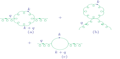
Figure 2: The graviton((a),(b)) and its ghost((c)) one-loop contributions to the graviton propagator. $q$ is the 4-momentum of the graviton.

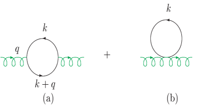
Figure 3: The scalar one-loop contribution to the graviton propagator. $q$ is the 4-momentum of the graviton.

For example, consider the graph in Fig. 3a. When we use our resummed propagators, we get (here, $k\rightarrow(ik^{0},\vec{k})$ by Wick rotation, and we work in the transverse-traceless space)

$$\begin{split}i\Sigma(q)^{1a}_{\bar{\mu}\bar{\nu};\mu\nu}&=i\kappa^{2}\frac{\int d^{4}k}{2(2\pi)^{4}}\frac{\left(k^{\prime}_{\bar{\mu}}k_{\bar{\nu}}+k^{\prime}_{\bar{\nu}}k_{\bar{\mu}}\right)e^{\frac{\kappa^{2}|{k^{\prime}}^{2}|}{8\pi^{2}}\ln\left(\frac{m^{2}}{m^{2}+|{k^{\prime}}^{2}|}\right)}}{\left({k^{\prime}}^{2}-m^{2}+i\epsilon\right)}\\ &\qquad\frac{\left(k^{\prime}_{\mu}k_{\nu}+k^{\prime}_{\nu}k_{\mu}\right)e^{\frac{\kappa^{2}|k^{2}|}{8\pi^{2}}\ln\left(\frac{m^{2}}{m^{2}+|k^{2}|}\right)}}{\left(k^{2}-m^{2}+i\epsilon\right)}.\end{split}$$ (70)

We see explicitly that the exponential damping in the deep Euclidean regime has rendered the graph in Fig. 3a finite in the UV. For the same reason, all of the graphs in Figs. 2 and 3 are UV finite when we use our respective resummed propagators to compute them.

To evaluate the effect of the corrections in Figs. 2 and 3 on the graviton propagator, we continue to work in the transverse, traceless space and isolate the effects from Figs. 2 and 3 on the coefficient of the $q^{4}$ in the graviton propagator denominator,

$$q^{2}+\frac{1}{2}q^{4}\Sigma^{T(2)}+i\epsilon,$$ (71)

so that we need to evaluate the transverse, traceless self-energy function $\Sigma^{T}(q^{2})$ that follows from (70) for Fig. 3a and its analogs for Figs. 3b and 2 by the standard methods. Here, we work in the expectation that, in consequence to the newly UV finite calculated quantum loop effects in Figs. 2 and 3, the Fourier transform of the graviton propagator that enters Newton’s law, our ultimate goal here, will receive support from from $|q|^{2}<<M_{Pl}^{2}$. We will therefore work in the limit that $q^{2}/M_{Pl}^{2}$ is relatively small, $\lesssim.1$, for example . This will allow us to see the dominant effects of our new finite quantum loop effects. In other words, we will work to $\sim 10\%$ (leading-log) accuracy in what follows. See Appendix 2 for more discussion on this point.

First let us dispense with the contributions from Figs. 2b and Fig. 3b. These are independent of $q^{2}$ so that we use a mass counter-term to remove them and set the graviton mass to $0$. Following the suggestion of Feynman in Ref. [33], we will change this to a small non-zero value below to take into account the recently established small value of the cosmological constant [29, 30]. See also the discussion in Ref. [67, 68, 69, 70] where it is shown that the quantum fluctuations in the exact de Sitter metric implied by the non-zero cosmological constant correspond in general to a mass for the graviton. Here, as we expand about a flat background, we take this effect into account as a small infrared regulator for the graviton. The deviations from flat space in the deep Euclidean region that we study due to the observed value of the cosmological constant are at the level of $e^{10^{-61}}-1$! This is safely well beyond the accuracy of our methods.

Returning to Fig. 3a, when we project onto the transverse, traceless space, that is to say, the graviton helicity space $\{e^{\mu\nu}(\pm 2)=\epsilon^{\mu}_{\pm}\epsilon^{\nu}_{\pm},\,\text{where}\,\epsilon^{\nu}_{\pm}=\pm(\hat{x}\pm i\hat{y})/\sqrt{2}\,\text{when}\,\\ \hat{x},~{}\hat{y}\,\text{are purely space-like and}(\vec{\hat{x}},\vec{\hat{y}},\vec{q}/|\vec{q}|)\,\text{form a right-handed coordinate basis}\}$, we get (see the Appendix 3) the result

$$i\Sigma^{T}(q^{2})_{3a}=\frac{-i\kappa^{2}m^{4}}{96\pi^{2}}\int^{1}_{0}d\alpha\int^{\infty}_{0}dx\frac{x^{3}(2(x+1)\bar{d}+\bar{d}^{2})}{(x+1)^{2}(x+1+\bar{d})^{2}}(1+x)^{-\lambda_{c}x}$$ (72)

where $\lambda_{c}=\frac{2m^{2}}{\pi M_{Pl}^{2}}$, $\bar{d}=\alpha(1-\alpha)\vec{q}^{2}/m^{2}$ so that we have made the substitution $x=k^{2}$ and imposed the mass counter-term as we noted. We have taken for definiteness $q=(0,\vec{q})$. We also use $q=|\vec{q}|$ when there is no chance for confusion. We are evaluating (72) in the deep UV where $m^{2}/q^{2}<<1$ and where $q^{2}/M_{Pl}^{2}\lesssim 0.1$ – see footnote 8. Accordingly, we get

$$i\Sigma^{T}(q^{2})_{3a}=\frac{-i\kappa^{2}}{96\pi^{2}}\left(\frac{|\vec{q}|^{2}m^{2}c_{1}}{3}+\frac{|\vec{q}|^{4}c_{2}}{30}\right)$$ (73)

where

$$\begin{split}c_{1}=I_{1}(\lambda_{c})&=\int^{\infty}_{0}dxx^{3}(1+x)^{-3-\lambda_{c}x}\\ c_{2}=I_{2}(\lambda_{c})&=\int^{\infty}_{0}dxx^{3}(1+x)^{-4-\lambda_{c}x}.\end{split}$$ (74)

Using the usual field renormalization, we see that Fig. 3a makes the contribution

$$i\tilde{\Sigma}^{T}(q^{2})_{3a}\cong\frac{-i\kappa^{2}|\vec{q}|^{4}c_{2}}{2880\pi^{2}}$$ (75)

to the transverse traceless graviton proper self-energy function.

Turning now to Figs. 2, the pure gravity loops, we use a contact between our work and that of Refs. [47]. In Refs. [47], the entire set of one-loop divergences has been computed for the theory in (6). The basic observation is the following. As we work only to the leading logarithmic accuracy in $\ln\lambda_{c}$, it is sufficient to identify the correspondence between the divergences as calculated in the n-dimensional regularization scheme in Ref. [47] and as they would occur when $\lambda_{c}\rightarrow 0$. This we do by comparing our result for (72) when $q^{2}\rightarrow 0$ with the corresponding result in Ref. [47] for the same theory. In this way we see that we have the correspondence

$$-\ln\lambda_{c}\leftrightarrow\frac{1}{2-n/2}.$$ (76)

This allows us to read-off the leading log result for the pure gravity loops directly from the results in Ref. [47]. Since $-\ln\lambda_{c}=\ln{M_{Pl}}^{2}-\ln m^{2}-\ln\frac{2}{\pi}$, we see that our exponentiated propagators have cut-off our UV divergences at the scale $\sim M_{Pl}$ and the correspondence in (76) shows the usual relation between the effective UV cut-off scale and the pole in $(2-n/2)$ in dimensional regularization. Note as well that, if the small cosmological constant[29, 30] is set to zero , the graviton is then exactly massless and we normalize its propagator at a Euclidean point $p^{2}=-\mu^{2}$ as is standard for massless non-Abelian gauge theories for example. It follows that for the graviton case and for all other cases where $m=0$, as we explain in Appendix 1 (see (69)), the mass $m$ in (76) is replaced with $m=\mu$ – there is no zero mass divergence in the case that the mass of the respective particle is zero. The UV correspondence is the same in both the $m\neq 0$ and $m=0$ cases.

Specifically, the result in Ref. [47], when interpreted as we have just explained, is that the pure gravity loops give a factor of 42 times the scalar loops for the coefficient $a_{2}$ above when we work in the regime where $|q^{2}|$ is relatively small compared to $M_{Pl}^{2}$. Here, we again take into account the recent evidence for a non-zero cosmological constant [29, 30], which can be seen to provide the small non-zero rest mass for the graviton, $m_{g}\cong 3.1\times 10^{-33}$eV, which serves as an IR regulator for the graviton. This is the value of rest mass in $\lambda_{c}$ which should be used for pure gravitational loops – see footnote 9 for more discussion on this point relevant to Refs. [71, 72]. See the Appendix 1 for the derivation of the corresponding infrared exponents.

We note that, for $\lambda_{c}=0$, the constant $c_{2}$ is infinite and, as we have already imposed both the mass and field renormalization counter-terms, there would be no physical parameter into which that infinity could be absorbed: this is just another manifestation that QGR, without our resummation, is a non-renormalizable theory.

Using the universality of the coupling of the graviton when the momentum transfer scale is relatively small compared to $M_{Pl}$, we can extend the result for the scalar field above to the remaining known particles in the Standard Model by counting the number of physical degrees of freedom for each such particle and replacing the mass of the scalar with the respective mass of that particle. For a massive fermion we get a factor of 4 relative to the scalar result with the appropriate change in the mass parameter from $m$ to $m_{f}$, the mass of that fermion, for a massive vector, we get a factor of 3 relative to the scalar result, with the corresponding change in the mass from $m$ to $m_{V}$, the mass of that vector, etc. In this way, we arrive at the result that the denominator of the graviton propagator becomes, in the Standard Model,

$$q^{2}+\Sigma^{T}(q^{2})+i\epsilon\cong q^{2}-q^{4}\frac{c_{2,eff}}{360\pi M_{Pl}^{2}},$$ (77)

where we have defined

$$\begin{split}c_{2,eff}&=\sum_{\text{SM particles j}}n_{j}I_{2}(\lambda_{c}(j))\\ &\cong 2.56\times 10^{4}\end{split}$$ (78)

with $I_{2}$ defined above and with $\lambda_{c}(j)=\frac{2m_{j}^{2}}{\pi M_{Pl}^{2}}$ and [12] $n_{j}$ equal to the number of effective degrees of particle $j$ as already illustrated. The values for Standard Model masses used in arriving at the numerical value for $c_{2,eff}$ in (78) are explained in the text. We also note that (see Appendix 3) for $\lambda_{c}\rightarrow 0$, we have found the approximate representation

$$I_{2}(\lambda_{c})\cong\ln\frac{1}{\lambda_{c}}-\ln\ln\frac{1}{\lambda_{c}}-\frac{\ln\ln\frac{1}{\lambda_{c}}}{\ln\frac{1}{\lambda_{c}}-\ln\ln\frac{1}{\lambda_{c}}}-\frac{11}{6}.$$ (79)

The results (77), (78) and (79) have been used in the text.

Appendix 3: Evaluation of Gravitationally Regulated Loop Integrals

In this section we present the derivation of the representations which we have used in the text in evaluating the gravitationally regulated loop integrals in Figs. 2,3.

Considering the integrals in Fig. 3 to show the methods, we need the result for

$$\begin{split}{\cal I}_{\bar{\mu}\bar{\nu};\mu\nu}&=i\frac{\int d^{4}k}{(2\pi)^{4}}\frac{\left(k^{\prime}_{\bar{\mu}}k_{\bar{\nu}}+k^{\prime}_{\bar{\nu}}k_{\bar{\mu}}\right)e^{\frac{\kappa^{2}|{k^{\prime}}^{2}|}{8\pi^{2}}\ln\left(\frac{m^{2}}{m^{2}+|{k^{\prime}}^{2}|}\right)}}{\left({k^{\prime}}^{2}-m^{2}+i\epsilon\right)}\\ &\qquad\frac{\left(k^{\prime}_{\mu}k_{\nu}+k^{\prime}_{\nu}k_{\mu}\right)e^{\frac{\kappa^{2}|k^{2}|}{8\pi^{2}}\ln\left(\frac{m^{2}}{m^{2}+|k^{2}|}\right)}}{\left(k^{2}-m^{2}+i\epsilon\right)}.\end{split}$$ (80)

In the limit that $|q^{2}|<<M_{Pl}^{2}$, standard symmetric integration methods give us, for the transverse parts,

$${\cal I}_{\bar{\mu}\bar{\nu};\mu\nu}=\frac{i\pi^{2}}{12}\{g_{\bar{\mu}\bar{\nu}}g_{\mu\nu}+permutations\}I_{0}$$ (81)

where we have

$$I_{0}\cong\frac{\int_{0}^{1}d\alpha\int_{0}^{\infty}dkk^{3}}{(2\pi)^{4}}\frac{k^{4}e^{\lambda_{c}(k^{2}/m^{2})\ln(m^{2}/(m^{2}+k^{2}))}}{[k^{2}+m^{2}+|q^{2}|\alpha(1-\alpha)]^{2}}$$ (82)

and where we used the symmetrization, valid under the respective integral sign,

$$k_{\bar{\mu}}k_{\bar{\nu}}k_{\mu}k_{\nu}\rightarrow\frac{k^{4}}{24}\{g_{\bar{\mu}\bar{\nu}}g_{\mu\nu}+permutations\}$$ (83)

and $\lambda_{c}=2m^{2}/(\pi M_{Pl}^{2})$. The integral $I_{0}$, with the use of the mass counter-term, then leads us to evaluate the difference,

$$\Delta I=I_{0}(q)-I_{0}(0)\cong\frac{\int_{0}^{1}d\alpha\int_{0}^{\infty}dx}{2(2\pi)^{4}}\frac{x^{3}(x+1)^{-\lambda_{c}x}}{(x+1)^{2}(x+1+\bar{d})^{2}}\left(-2\bar{d}(x+1)-\bar{d}^{2}\right)$$ (84)

where we define here $\bar{d}=|q^{2}|\alpha(1-\alpha)/m^{2}$. It is seen that the dominant part of the integrals comes from the regime where $x\sim 1/(\rho\lambda_{c})$ with $\rho=-\ln\lambda_{c}$, so that we may finally write

$$\begin{split}\Delta I&=I_{0}(q)-I_{0}(0)\\ &\cong\frac{\int_{0}^{1}d\alpha\int_{0}^{\infty}dx}{2(2\pi)^{4}}\frac{x^{3}(x+1)^{-\lambda x}}{(x+1)^{2}(x+1+\bar{d})^{2}}\left(-2\bar{d}(x+1)-\bar{d}^{2}\right)\\ &\cong-\frac{|q|^{2}I_{1}}{6(2\pi)^{4}}-\frac{|q|^{4}I_{2}}{60(2\pi)^{4}}\end{split}$$ (85)

where we have defined

$$\begin{split}I_{1}(\lambda_{c})&=\int^{\infty}_{0}dxx^{3}(1+x)^{-3-\lambda_{c}x},\\ I_{2}(\lambda_{c})&=\int^{\infty}_{0}dxx^{3}(1+x)^{-4-\lambda_{c}x}.\end{split}$$

The result (85) has been used in the text.

For the limit in practice, where we have $\lambda_{c}\rightarrow 0$, we can get accurate estimates for the integrals $I_{1},I_{2}$ as follows. Consider first $I_{2}$. Write $x^{3}=(x+1-1)^{3}=(x+1)^{3}-3(x+1)^{2}+3(x+1)-1$ to get

$$\begin{split}I_{2}(\lambda_{c})&=\int^{\infty}_{0}dx\left((1+x)^{-1}-3(x+1)^{-2}+3(x+1)^{-3}-(x+1)^{-4}\right)(1+x)^{-\lambda_{c}x}\\ &\cong\int^{\infty}_{0}dx(x+1)^{-1-\lambda_{c}x}-\frac{11}{6}.\end{split}$$

Use then the change of variable $r=\lambda_{c}x$ to get, for $\rho=\ln(1/\lambda_{c})$,

$$\begin{split}\int^{\infty}_{0}dx(x+1)^{-1-\lambda_{c}x}&=\int^{\infty}_{0}dr\frac{e^{-r\ln(r+\lambda_{c})-\rho r}}{r+\lambda_{c}}\\ &=-\ln\lambda_{c}+\int^{\infty}_{0}dr\ln(r+\lambda_{c})(\ln(r+\lambda_{c})+r/(r+\lambda_{c})+\rho)e^{-r\ln(r+\lambda_{c})-\rho r}\\ &\cong\rho+\int^{\infty}_{0}dr\sum_{j=0}^{\infty}\frac{1}{j!}((\rho+1)(\partial/\partial\alpha)^{j+1}+(\partial/\partial\alpha)^{j+2})(\partial/\partial\rho)^{j}r^{\alpha}e^{-\rho r}|_{\alpha=0}\\ &=\rho+\sum_{j=0}^{\infty}\frac{1}{j!}((\rho+1)(\partial/\partial\alpha)^{j+1}+(\partial/\partial\alpha)^{j+2})(\partial/\partial\rho)^{j}\Gamma(\alpha+1)\rho^{-\alpha-1}|_{\alpha=0}\\ &\cong\rho+\frac{-(\rho+1)\ln\rho+\ln^{2}\rho}{\rho-\ln\rho}\\ &=\rho-\ln\rho-\frac{\ln\rho}{\rho-\ln\rho}.\end{split}$$ (86)

This gives us the approximation

$$I_{2}(\lambda_{c})=\rho-\ln\rho-\frac{\ln\rho}{\rho-\ln\rho}-\frac{11}{6}$$ (87)

when $\lambda_{c}\rightarrow 0$, as we noted in the text.

The integral $I_{1}$ is a field renormalization constant so, in the usual renormalization program, we do not need it for most of the applications. Here, we will discuss it as well for completeness. We get

$$\begin{split}I_{1}(\lambda_{c})&=\int_{0}^{\infty}dx(1+x)^{-\lambda_{c}x}-3\left(I_{2}(\lambda_{c})+\frac{11}{6}\right)+\frac{5}{2}\\ &=\int_{0}^{\infty}dx(1+x)^{-\lambda_{c}x}-3I_{2}(\lambda_{c})-3,\end{split}$$

where, as above, we use

$$\begin{split}\int_{0}^{\infty}dx(1+x)^{-\lambda_{c}x}&=\frac{\int_{0}^{\infty}dr}{\lambda_{c}}e^{-r\ln(r+\lambda_{c})-r\rho}\\ &\cong\frac{\int_{0}^{\infty}dr}{\lambda_{c}}\sum_{j=0}^{\infty}\frac{1}{j!}(\partial/\partial\rho)^{j}(\partial/\partial\alpha)^{j}r^{\alpha}e^{-\rho r}|_{\alpha=0}\\ &=\frac{1}{\lambda_{c}}\sum_{j=0}^{\infty}\frac{1}{j!}(\partial/\partial\rho)^{j}(\partial/\partial\alpha)^{j}\Gamma(1+\alpha)\rho^{-\alpha-1}|_{\alpha=0}\\ &\cong\frac{1}{\lambda_{c}}\frac{1}{\rho-\ln\rho}.\end{split}$$

Thus, we get

$$I_{1}(\lambda_{c})\cong\frac{1}{\lambda_{c}}\frac{1}{\rho-\ln\rho}-3I_{2}(\lambda_{c})-3.$$ (88)

Finally, let us show why we can neglect the terms $\bar{d}$ that were in the denominators of $I_{j},~{}j=1,2$. It is enough to look into the differences

$$\Delta I_{j}=\frac{\int_{0}^{\infty}dxx^{3}}{(x+1)^{j}}\left(\frac{1}{(x+1)^{2}}-\frac{1}{(x+1+\bar{d})^{2}}\right)(x+1)^{-\lambda_{c}x},~{}j=1,2$$ (89)

where we note that the integral $I_{1}$ is absorbed by the standard field renormalization where here for convenience we do this at $|q^{2}|=0$ when we neglect $\bar{d}$ in the denominator of $I_{1}$ or at the zero of the respective graviton propagator away from the origin otherwise. From this perspective, the main integral to examine to illustrate the level of our approximation becomes

$$\begin{split}\Delta I_{2}&=\frac{\int_{0}^{\infty}dx}{(x+1)^{2}}\{\frac{(x+1)^{-\lambda_{c}x}}{(x+1)^{2}}-\frac{(x+1)^{-\lambda_{c}x}}{(x+1+\bar{d})^{2}}\}\\ &=\frac{\int_{0}^{\infty}dr\,e^{-r\ln(r+\lambda_{c})-r\rho}}{(r+\lambda_{c})^{2}}\{\frac{1}{(r+\lambda_{c})^{2}}-\frac{1}{(r+\lambda_{c}+\sigma)^{2}}\}\\ &\cong\int_{0}^{\infty}dr\int_{0}^{\infty}d\alpha_{1}\alpha_{1}\int_{0}^{\infty}d\alpha_{2}\alpha_{2}e^{-r\ln r-r\rho-\alpha_{1}(r+\lambda_{c})-\alpha_{2}(r+\lambda_{c})}\left(1-e^{-\alpha_{2}\sigma}\right),\end{split}$$ (90)

where we have defined $\sigma=\lambda_{c}\bar{d}$. The approximation, valid for small values of $\sigma$,

$$\begin{split}\left(1-e^{-\alpha_{2}\sigma}\right)&=2e^{-\alpha_{2}\sigma/2}\sinh(\alpha_{2}\sigma/2)\\ &\cong\alpha_{2}\sigma e^{-\alpha_{2}\sigma/2}\end{split}$$ (91)

then allows us to get

$$\begin{split}\Delta I_{2}&\cong 4\sigma\frac{\partial^{2}}{\partial\sigma^{2}}\int_{0}^{\infty}dr\,e^{-r\rho}\left(1-\frac{\lambda_{c}+\sigma/2}{r+\lambda_{c}+\sigma/2}\right)\\ &\cong 2+\rho\sigma+2\rho\sigma(1+\frac{1}{4}\rho\sigma)e^{\rho\sigma/2}(C+\ln(\rho\sigma/2)+\sum_{n=1}^{\infty}\frac{(-1)^{n}(\rho\sigma/2)^{n}}{n\;n!})\\ \end{split}$$ (92)

which shows that this difference is indeed non-leading log. The analogous analysis holds for $\Delta I_{1}$ as well.

References

• [1] S. Weinberg, in General Relativity, an Einstein Centenary Survey, eds. S. W. Hawking and W. Israel, (Cambridge Univ. Press, Cambridge, 1979).
• [2] M. Reuter, Phys. Rev. D57 (1998) 971, and references therein.
• [3] O. Lauscher and M. Reuter, Phys. Rev. D66 (2002) 025026, and references therein.
• [4] E. Manrique, M. Reuter and F. Saueressig, Ann. Phys. 326 (2011) 44 and references therein.
• [5] A. Bonanno and M. Reuter, Phys. Rev. D62 (2000) 043008, and references therein.
• [6] D. F. Litim, Phys. Rev. Lett.92(2004) 201301; Phys. Rev. D64 (2001) 105007; P. Fischer and D.F. Litim, Phys. Lett. B638 (2006) 497 and references therein.
• [7] D. Don and R. Percacci, Class. Quant. Grav. 15 (1998) 3449; R. Percacci and D. Perini, Phys. Rev. D67(2003) 081503; ibid.68 (2003) 044018; R. Percacci, ibid.73(2006) 041501; A. Codello, R. Percacci and C. Rahmede, Int.J. Mod. Phys. A23(2008) 143, and references therein.
• [8] K. G. Wilson, Phys. Rev. B4 (1971) 3174, 3184; K. G. Wilson, J.Kogut, Phys. Rep. 12 (1974) 75; F. Wegner, A. Houghton, Phys. Rev. A8(1973) 401; S. Weinberg, “Critical Phenomena for Field Theorists”, Erice Subnucl. Phys. (1976) 1; J. Polchinski, Nucl. Phys. B231 (1984) 269.
• [9] B.F.L. Ward, Open Nucl.Part.Phys.Jour. 2(2009) 1.
• [10] B.F.L. Ward, Mod. Phys. Lett. A17 (2002) 237.
• [11] B.F.L. Ward, Mod. Phys. Lett. A19 (2004) 143.
• [12] B.F.L. Ward, J. Cos. Astropart. Phys.0402 (2004) 011.
• [13] B.F.L. Ward, hep-ph/0605054, Acta Phys. Polon. B37 (2006) 1967.
• [14] B.F.L. Ward, hep-ph/0503189, Acta Phys. Polon. B37 (2006) 347.
• [15] B.F.L. Ward, hep-ph/0502104, in Focus on Black Hole Research, ed. P.V. Kreitler,(Nova Sci. Publ., Inc., New York, 2006) p. 95.
• [16] B.F.L. Ward, hep-ph/0411050, Int. J. Mod. Phys. A20 (2005) 3502.
• [17] B.F.L. Ward, hep-ph/0411049, Int. J. Mod. Phys. A20 (2005) 3128.
• [18] B.F.L. Ward, hep-ph/0410273, in Proc. ICHEP 2004, vol. 1, eds. H. Chen et al.,(World Sci. Publ. Co., Singapore, 2005) p. 419 and references therein.
• [19] B.F.L. Ward, Mod. Phys. Lett. A23 (2008) 3299.
• [20] D. R. Yennie, S. C. Frautschi, and H. Suura, Ann. Phys. 13 (1961) 379; see also K. T. Mahanthappa, Phys. Rev. 126 (1962) 329, for a related analysis.
• [21] See also S. Jadach and B.F.L. Ward, Comput. Phys. Commun. 56(1990) 351; Phys.Lett. B274 (1992) 470; S. Jadach et al., Comput. Phys. Commun. 102 (1997) 229; S. Jadach, W. Placzek and B.F.L Ward, Phys. Lett. B390 (1997) 298; S. Jadach, M. Skrzypek and B.F.L. Ward,Phys. Rev. D 55 (1997) 1206; S. Jadach, W. Placzek and B.F.L. Ward, Phys. Rev. D 56 (1997) 6939; S. Jadach, B.F.L. Ward and Z. Was,Phys. Rev. D 63 (2001) 113009; Comp. Phys. Commun. 130 (2000) 260; ibid.124 (2000) 233; ibid.79 (1994) 503; ibid.66 (1991) 276; S. Jadach et al., ibid.140 (2001) 432, 475.
• [22] J. Ambjorn et al., Phys. Lett. B690 (2010) 420, and references therein.
• [23] P. Horava, Phys. Rev. D 79 (2009) 084008.
• [24] A. Bonanno and M. Reuter, Phys. Rev. D65 (2002) 043508.
• [25] A. Bonanno and M. Reuter, Jour. Phys. Conf. Ser. 140 (2008) 012008, arXiv:0803.2546; and references therein.
• [26] I. L. Shapiro and J. Sola, Phys. Lett. B475 (2000) 236.
• [27] See for example A. H. Guth and D.I. Kaiser, Science 307 (2005) 884; A. H. Guth, Phys. Rev. D23 (1981) 347, and references therein.
• [28] See for example A. Linde, Lect. Notes. Phys. 738 (2008) 1, and references therein.
• [29] A.G. Riess et al., Astron. Jour. 116 (1998) 1009; S. Perlmutter et al., Astrophys. J. 517 (1999) 565; and, references therein.
• [30] C. Amsler et al., Phys. Lett. B667 (2008) 1.
• [31] B.F.L. Ward, to appear.
• [32] R.P. Feynman, Acta Phys. Pol.24 (1963) 697-722.
• [33] R.P. Feynman, Feynman Lectures on Gravitation, eds. F.B. Moringo and W.G. Wagner,(Caltech, Pasadena, 1971).
• [34] L.D. Faddeev and V.N. Popov, “Perturbation theory for gauge invariant fields”, preprint ITF-67-036, NAL-THY-57 (translated from Russian by D. Gordon and B.W. Lee). Available from http://lss.fnal.gov/archive/test-preprint/fermilab-pub-72-057-t.shtml.
• [35] L.D. Faddeev and V.N. Popov, Phys. Lett. B25 (1967) 29-30.
• [36] S. Weinberg, The Quantum Theory of Fields, v.1,(Cambridge University Press, Cambridge, 1995).
• [37] G. ’t Hooft and M. Veltman, Nucl. Phys. B44(1972) 189, and references therein.
• [38] J.D. Bjorken and S.D. Drell, Relativistic Quantum Fields,(McGraw-Hill, Menlo Park, 1965).
• [39] See for example D. Wark, in Proc. ICHEP02, eds. S. Bentvelsen et al., (North-Holland,Amsterdam, 2003), Nucl. Phys. B (Proc. Suppl.) 117 (2003) 164.
• [40] See for example M. C. Gonzalez-Garcia, hep-ph/0211054, in Proc. ICHEP02, eds. S. Bentvelsen et al., (North-Holland,Amsterdam, 2003), Nucl. Phys. B (Proc. Suppl.) 117 (2003) 186, and references therein.
• [41] K. Hagiwara et al., Phys. Rev. D66 (2002) 010001.
• [42] H. Leutwyler and J. Gasser, Phys. Rept. 87 (1982) 77, and references therein.
• [43] S. Eidelman et al., Phys. Lett. B592 (2004) 1.
• [44] D. Abbaneo et al., hep-ex/0212036.
• [45] M. Gruenewald, hep-ex/0210003, in Proc. ICHEP02, eds. S. Bentvelsen et al., (North-Holland,Amsterdam, 2003), Nucl. Phys. B Proc. Suppl. 117(2003) 280.
• [46] F. Gianotti, in Proc. ICHEP2012, in press; J. Incandela, ibid., 2012, in press; G. Aad et al., Phys. Lett. B716 (2012) 1; S. Chatrchyan et al., Phys. Lett. B716 (2012) 30.
• [47] G. ’t Hooft and M. Veltman, Ann. Inst. Henri Poincare XX (1974) 69.
• [48] Ya. B. Zeldovich, Sov. Phys. Uspekhi 11 (1968) 381.
• [49] V. Branchina and D. Zappala, G. R. Gravit. 42 (2010) 141; arXiv:1005.3657, and references therein.
• [50] J. Sola, J. Phys. A41 (2008) 164066.
• [51] T. Appelquist and J. Carazzone, Phys. Rev. D11 (1975) 2856.
• [52] S.L. Glashow, Nucl. Phys. 22 (1961) 579; S. Weinberg, Phys. Rev. Lett. 19 (1967) 1264; A. Salam, in Elementary Particle Theory, ed. N. Svartholm (Almqvist and Wiksells, Stockholm, 1968), p. 367; G. ’t Hooft and M. Veltman, Nucl. Phys. B44,189 (1972) and 50, 318 (1972); G. ’t Hooft, ibid. 35, 167 (1971); M. Veltman, ibid. 7, 637 (1968).
• [53] D. J. Gross and F. Wilczek, Phys. Rev. Lett. 30 (1973) 1343; H. David Politzer, ibid.30 (1973) 1346; see also , for example, F. Wilczek, in Proc. 16th International Symposium on Lepton and Photon Interactions, Ithaca, 1993, eds. P. Drell and D.L. Rubin (AIP, NY, 1994) p. 593, and references therein.
• [54] S. Bethke, Eur. Phys. J. C64 (2009) 689.
• [55] P.S. Bhupal Dev and R.N. Mohapatra, Phys. Rev. D82 (2010) 035014, and references therein.
• [56] See for example H.E. Haber and G.L. Kane, Phys. Rep.117 (1985) 75, and references therein.
• [57] See for example S. Lowette, in Proc. Rencontres de Moriond EW 2012, in press, and references therein.
• [58] See for example G. Stiegman, Ann. Rev. Nucl. Part. Sci.57 (2007) 463, and references therein.
• [59] S. Basilakos, M. Plionis and J. Sola, arXiv:0907.4555.
• [60] J. Grande et al., J. Cos. Astropart. Phys. 1108 (2011) 007, arXiv:1103.4632.
• [61] H. Fritzsch and J. Sola, arXiv:1202.5097, and references therein.
• [62] R.K. Ellis et al., Phys. Lett. B78 (1978) 281-4.
• [63] R.K. Ellis et al., Nucl. Phys. B152 (1979) 285-329.
• [64] D. Amati, R. Petronzio and G. Veneziano G, Nucl. Phys. Bbf 146 (1978) 29-49.
• [65] S. Libby and G. Sterman G, Phys. Rev. D18 (1978) 3252-68.
• [66] A. Mueller, Phys. Rev. D18 (1978) 3705-27.
• [67] M. Novello, R.P. Neves, Class. Quant. Grav.20 (2003) L67-73.
• [68] M. Novello and R.P. Neves, Class. Quant. Grav.19(2002) 5335-51.
• [69] J.P. Gazeau and M. Novello, arXiv.org:/gr-qc/0610054.
• [70] M. Novello M, in Proc. 5th International Conference on Mathematical Methods in Physics, eds. J.A.H Neto and A.A. Bytsenko, PoS IC2006 (2006) 009.
• [71] H. van Dam and M. Veltman, Nucl. Phys. B22 (1970) 397-411.
• [72] V.I. Zakharov, Pisma Zh. Eksp. Teor. Fiz. 12 (1970) 447-449.