Dynamics of nodal points and the nodal count on a family of quantum graphs

Abstract.

We investigate the properties of the zeros of the eigenfunctions on quantum graphs (metric graphs with a Schrödinger-type differential operator). Using tools such as scattering approach and eigenvalue interlacing inequalities we derive several formulas relating the number of the zeros of the $n$-th eigenfunction to the spectrum of the graph and of some of its subgraphs. In a special case of the so-called dihedral graph we prove an explicit formula that only uses the lengths of the edges, entirely bypassing the information about the graph’s eigenvalues. The results are explained from the point of view of the dynamics of zeros of the solutions to the scattering problem.

1. Introduction

Spectral properties of differential operators on graphs have recently arisen as models for such diverse areas of research as quantum chaos, photonic crystals, quantum wires and nanostructures. We refer the interested reader to the reviews [1, 2] as well as to collections of recent results [3, 4]. As a part of this research program, the study of eigenfunctions, and in particular, their nodal domains is an exciting and rapidly developing research direction. It is an extension to graphs of the investigations of nodal domains on manifolds, which started already in the 19th century by the pioneering work of Chladni on the nodal structures of vibrating plates. Counting nodal domains started with Sturm’s oscillation theorem which states that a vibrating string is divided into exactly $n$ nodal intervals by the zeros of its $n$-th vibrational mode. In an attempt to generalize Sturm’s theorem to manifolds in more than one dimension, Courant formulated his nodal domains theorem for vibrating membranes, which bounds the number of nodal domains of the $n$-th eigenfunction by $n$ [5]. Pleijel has shown later that Courant’s bound can be realized only for finitely many eigenfunctions [6]. The study of nodal domains counts was revived after Blum et al have shown that nodal count statistics can be used as a criterion for quantum chaos [7]. A subsequent paper by Bogomolny and Schmit illuminated the fascinating connection between nodal statistics and percolation theory [8]. A recent paper by Nazarov and Sodin addresses the counting of nodal domains of eigenfunctions of the Laplacian on $\mathbb{S}^{2}$ [9]. They prove that on average, the number of nodal domains increases linearly with $n$, and the variance about the mean is bounded. At the same time, it was shown that the nodal sequence - the sequence of numbers of nodal domains ordered by the corresponding spectral parameters - stores geometrical information about the domain [10]. Moreover, there is a growing body of numerical and theoretical evidence which shows that the nodal sequence can be used to distinguish between isospectral manifolds [11, 12, 13].

As far as counting nodal domains on graphs is concerned, it has been shown that trees behave as one-dimensional manifolds, and the analogue of Sturm’s oscillation theory applies [14, 15, 16, 17], as long as the eigenfunction does not vanish at any vertex. Thus, denoting by $\nu_{n}$ the number of nodal domains of the $n$’th eigenfunction, one has $\nu_{n}=n$ for tree graphs. Courant’s theorem applies for the eigenfunctions on a generic graph: $\nu_{n}\leq n$, [18]. It should be noted that there is a correction due to multiplicity of the $n$-th eigenvalue and the upper bound becomes $n+m-1$, where $m$ is the multiplicity [19]. In addition, a lower bound for the number of nodal domains was discovered recently. It is shown in [20] that the nodal domains count of the $n$-th eigenfunction has no less than $n-\beta$ nodal domains, where $\beta$ is the number of independent cycles in the graph. Again, this result is valid for generic eigenfunctions, namely, the eigenfunction has no zero entries on the vertices and belongs to a simple eigenvalue. In a few cases, the nodal counts of isospectral quantum graphs were shown to be different, and thus provided further support to the conjecture that nodal count resolves isospectrality [21]. A recent review entitled “Nodal domains on graphs - How to count them and why?" [22] provides a detailed answer to the question which appears in its title (as it was known when the article was written). In particular, this manuscript contains a numerically established formula for the nodal count of a specific quantum graph, expressed in terms of the lengths of its edges. This was the first, and to this date the only, explicit nodal count formula for a non-trivial graph and in this manuscript we succeed in rigorously proving it.

This leads us to focus on the study of nodal domains on quantum graphs from a new point of view. Namely, we shall show that one can count the number of nodal domains by using scattering data obtained by attaching semi-infinite leads to the graph. Scattering on graphs was proposed as a paradigm for chaotic scattering in [23, 24] with new applications and further developments in the field described in [25, 26, 27]. The work presented here is based on the concepts and ideas developed in these studies.

The paper is organized in the following way. The current section provides the necessary definitions and background from the theory of quantum graphs. The conversion of finite graphs to scattering systems by adding leads will be discussed in the next section and the expression for the scattering matrix will be derived and studied in detail. The connection of the scattering data with nodal domains and the counting methods it yields will be presented in section 3. Section 4 applies the above counting methods in order to derive a formula for the nodal count of graphs with disjoint cycles. This formula relates the nodal count to the spectra of the graph and some of its subgraphs. Thus, information about the eigenfunctions is exclusively obtained from the eigenvalue spectrum. The last section relates the different ways of counting and discusses possible future developments.

1.1. Quantum graphs

In this section we describe the quantum graph which is a metric graph with a Shrödinger-type self-adjoint operator defined on it. Let $\Gamma=(\mathcal{V},\mathcal{E})$ be a connected graph with vertices $\mathcal{V}=\{v_{j}\}$ and edges $\mathcal{E}=\{e_{j}\}$. The sets $\mathcal{V}$ and $\mathcal{E}$ are required to be finite.

We are interested in metric graphs, i.e. the edges of $\Gamma$ are $1$-dimensional segments with finite positive lengths $\{L_{e}\}_{e\in\mathcal{E}}$. On the edge $e=(u,v)$ we use two coordinates, $x_{e,v}$ and $x_{e,u}$. The coordinate $x_{e,v}$ measures the distance along the edge starting from the vertex $v$; $x_{e,u}$ is defined similarly. The two coordinates are connected by $x_{e,v}+x_{e,u}=L_{e}$. Sometimes, when the precise nature of the coordinate is unimportant, we will simply write $x_{e}$ or even $x$.

A metric graph becomes quantum after being equipped with an additional structure: assignment of a self-adjoint differential operator. This operator will be often called the Hamiltonian. In this paper we study the zeros of the eigenfunctions of the negative second derivative operator ($x$ is the coordinate along an edge)

(1.1) $$H\ :\ f(x)\mapsto-\frac{d^{2}f}{dx^{2}}.$$

or the more general Schrödinger operator

(1.2) $$H\ :\ f(x)\mapsto-\frac{d^{2}f}{dx^{2}}+V(x)f(x),$$

where $V(x)$ is a potential. Note that the value of a function or the second derivative of a function at a point on the edge is well-defined, thus it is not important which coordinate, $x_{e,v}$ or $x_{e,u}$ is used. This is in contrast to the first derivative which changes sign according to the direction of the chosen coordinate.

To complete the definition of the operator we need to specify its domain.

Definition 1.1.

We denote by $\widetilde{H}^{2}(\Gamma)$ the space

$$\widetilde{H}^{2}(\Gamma):=\bigoplus_{e\in\mathcal{E}}H^{2}(e),$$

which consists of the functions $f$ on $\Gamma$ that on each edge $e$ belong to the Sobolev space $H^{2}(e)$. The restriction of $f$ to the edge $e$ is denoted by $f_{e}$. The norm in the space $\widetilde{H}^{2}(\Gamma)$ is

$$\|f\|_{\widetilde{H}^{2}(\Gamma)}:=\sum\limits_{e\in\mathcal{E}}\|f_{e}\|^{2}_{H^{2}(e)}.$$

Note that in the definition of $\widetilde{H}^{2}(\Gamma)$ the smoothness is enforced along edges only, without any junction conditions at the vertices at all. However, the standard Sobolev trace theorem (e.g., [28]) implies that each function $f_{e}$ and its first derivative have well-defined values at the endpoints of the edge $e$. Since the direction is important for the first derivative, we will henceforth adopt the convention that, at an end-vertex of an edge $e$, the derivative is calculate into the edge and away from the vertex. That is the coordinate $x$ is chosen so that the vertex corresponds to $x=0$.

To complete the definition of the operator we need to specify its domain. All conditions that lead to the operator (1.1) being self-adjoint have been classified in [29, 30, 31]. We will only be interested in the so-called extended $\delta$-type conditions, since they are the only conditions that guarantee continuity of the eigenfunctions, something that is essential if one wants to study changes of sign of the said eigenfunctions.

Definition 1.2.

The domain $\mathcal{H}$ of the operator (1.2) consists of the functions $f\in\widetilde{H}^{2}(\Gamma)$ such that

1. $f$ is continuous on every vertex:

   (1.3) $$f_{e_{1}}(v)=f_{e_{2}}(v),$$

   for every vertex $v$ and edges $e_{1}$ and $e_{2}$ that have $v$ as an endpoint.

2. the derivatives of $f$ at each vertex $v$ satisfy

   (1.4) $$\sum_{e\in\mathcal{E}_{v}}\frac{df}{dx_{e}}(v)=\alpha_{v}f(v),\qquad\alpha_{v}\in\mathbb{R},$$

   where $\mathcal{E}_{v}$ is the set of edges incident to $v$.

Sometimes the condition (1.4) is written in a more robust form

(1.5) $$\cos(\gamma_{v})\sum_{e\in\mathcal{E}_{v}}\frac{df}{dx_{e}}(v)=\sin(\gamma_{v})f(v),$$

which is also meaningful for infinite values of $\alpha_{v}=\tan(\gamma_{v})$. Henceforth we will understand $\alpha_{v}=\infty$ as the Dirichlet condition $f(v)=0$. The case $\alpha_{v}=0$ is often referred to as the Neumann-Kirchhoff condition.

Finally, we will assume that the potential $V(x)$ is bounded and piecewise continuous. To summarize our discussion, the operator (1.2) with the domain $\mathcal{H}$ is self-adjoint for any choice of real $\alpha_{v}$. Since we only consider compact graphs, the spectrum is real, discrete and with no accumulation points. We will slightly abuse notation and denote by $\sigma(\Gamma)$ the spectrum of an operator $H$ defined on the graph $\Gamma$. It will be clear from the context which operator $H$ we mean and what are the vertex conditions.

The eigenvalues $\lambda\in\sigma(\Gamma)$ satisfy the equation

(1.6) $$-\frac{d^{2}f}{dx^{2}}+V(x)f(x)=\lambda f(x).$$

It can be shown that under the conditions specified above the operator $H$ is bounded from below [31]. Thus we can number the eigenvalues in the ascending order, starting with $1$. Sometimes we abuse the notation further and also call $k$, such that $\lambda=k^{2}$, an eigenvalue of the graph $\Gamma$. This also should lead to no confusion since, with the conditions $\mathrm{Re}(k)\geq 0$, $\mathrm{Im}(k)\geq 0$, the relation between $k$ and $\lambda$ is bijective.

1.2. Nodal count

The main purpose of this article is to investigate the number of zeros and the number of nodal domains of the eigenfunctions of a connected quantum graph. We aim to give formulas linking these quantities to the geometry of the graphs and to the eigenvalues of the graph and its subgraphs, but avoiding any reference to the values of the eigenfunctions themselves.

The number of internal zeros or nodal points of the function $f$ will be denoted by $\mu(f)$. We will use the shorthand $\mu_{n}$ to denote $\mu(f_{n})$ where $f_{n}$ is the $n$-th eigenfunction of the graph in question. The sequence $\{\mu_{n}\}$ will be called the nodal point count sequence. A positive (negative) domain with respect to $f$ is a maximal connected subset in $\Gamma$ where $f$ is positive (correspondingly, negative). The total number of positive and negative domains will be called the nodal domain count of $f$ and denoted by $\nu(f)$. Similarly to $\mu_{n}$, we use $\nu_{n}$ as a short-hand for $\nu(f_{n})$ and refer to $\{\nu_{n}\}$ as the nodal domain count sequence.

The two quantities $\mu_{n}$ and $\nu_{n}$ are closely related, although, due to the graph topology, the relationship is more complex than on a line, where $\nu=\mu+1$. Namely, one can easily establish the bound

(1.7) $$\mu-\beta_{\Gamma}+1\leq\nu\leq\mu+1,$$

where $\beta_{\Gamma}$ is the cyclomatic number of $\Gamma$. The cyclomatic number can be computed as

(1.8) $$\beta_{\Gamma}=|\mathcal{E}|-|\mathcal{V}|+1.$$

The cyclomatic number has several related interpretations: it counts the number of independent cycles in the graph (hence the name) and therefore it is the first Betti number of $\Gamma$ (hence the notation $\beta$). It also counts the minimal number of edges that need to be removed from $\Gamma$ to turn it into a tree. Correspondingly, $\beta_{\Gamma}=0$ if and only if $\Gamma$ is a tree.

There is another simple but useful observation relating the cycles on the graph and the number of zeros: if the eigenfunction of the graph does not vanish on the vertices of the graph, the number of zeros on any cycle of the graph is even. Indeed, an eigenfunction of a second order operator can only have simple zeros, thus at every zero $f$ changes sign. On a cycle there must be an even number of sign changes.

As mentioned earlier, we will be interested in the number of zeros and nodal domains of the eigenfunctions of operators (1.1) and (1.2) on graphs. According to the well known ODE theorem by Sturm [32, 33, 34], the zeros of the $n$-th eigenfunction of the operator of type (1.2) on an interval divide the interval into $n$ nodal domains. By contrast, in the corresponding question in $\mathbb{R}^{2}$ only an upper bound is possible, given by the Courant’s nodal line theorem [5], $\nu_{n}\leq n$. In a series of papers [14, 15, 18, 17, 20], it was established that a generic eigenfunction of the quantum graph satisfies both an upper and a lower bound. Namely, let $\lambda_{n}$ be a simple eigenvalue of $-\frac{d^{2}}{dx^{2}}+V(x)$ on a graph $\Gamma$ and its eigenfunction $f_{n}$ be non-zero at all vertices of $\Gamma$. Then the number of the nodal domains of $f_{n}$ satisfies

(1.9) $$n-\beta_{\Gamma}\leq\nu_{n}\leq n.$$

Similarly, for the number of zeros we have

(1.10) $$n-1\leq\mu_{n}\leq n-1+\beta_{\Gamma}.$$

Note that the upper bound in (1.10) follows from the upper bound in (1.9) and inequality (1.7). The lower bound in (1.10) requires an independent proof which is given in [35]. An interesting feature of quantum graphs is that, unlike the $\mathbb{R}^{d}$ case, the upper bound $\nu_{n}\leq n$ is in general not valid for degenerate eigenvalues.

In the present paper we combine these a priori bounds with scattering properties of a certain family of graphs to derive formulas for the nodal counts $\mu_{n}$ and $\nu_{n}$.

1.3. Quantum evolution map

When the potential $V(x)$ is equal to zero, the eigenvalue equation

(1.11) $$-\frac{d^{2}f}{dx^{2}}=k^{2}f(x),$$

has, on each edge, a solution that is a linear combination of the two exponents ${\mathrm{e}}^{\pm{\mathrm{i}}kx}$ if $k\neq 0$. We will write it in the form

(1.12) $$f_{e}(x_{e,v})=a_{e,v}^{\,in}\exp(-{\mathrm{i}}kx_{e,v})+a_{e,v}^{\,out}\exp({\mathrm{i}}kx_{e,v}),$$

where the variable $x_{e,v}$ measures the distance from the vertex $v$ of the edge $e$. The coefficient $a_{e,v}^{\,in}$ is the incoming amplitude on the edge $e$ (with respect to the vertex $v$) and $a_{e,v}^{\,out}$ is correspondingly the outgoing amplitude. However the same function can be expressed using the coordinate $x_{e,u}$ as

(1.13) $$f_{e}(x_{e,u})=a_{e,u}^{\,in}\exp(-{\mathrm{i}}kx_{e,u})+a_{e,u}^{\,out}\exp({\mathrm{i}}kx_{e,u}).$$

Since these two expressions should define the same function and since the two coordinates are connected, through the identity $x_{e,v}+x_{e,u}=L_{e}$, we arrive to the following relations

(1.14) $$a_{e,v}^{\,in}={\mathrm{e}}^{{\mathrm{i}}kL_{e}}a_{e,u}^{\,out}\qquad a_{e,u}^{\,in}={\mathrm{e}}^{{\mathrm{i}}kL_{e}}a_{e,v}^{\,out}$$

Fixing a vertex $v$ of degree $d_{v}$ and using (1.12) to describe the solution on the edges $\mathcal{E}_{v}$ adjacent to $v$ we obtain from (1.3) and (1.4) $d_{v}$ equations on the $2d_{v}$ variables $a_{e,v}^{\,out}$ and $a_{e,v}^{\,in}$. These equations can be rearranged as

(1.15) $$\vec{a}_{v}^{\,out}=\sigma^{(v)}(k)\vec{a}_{v}^{\,in},$$

where $\vec{a}_{v}^{\,out}$ and $\vec{a}_{v}^{\,in}$ are the vectors of the corresponding coefficients and $\sigma^{(v)}(k)$ is a $d_{v}\times d_{v}$ unitary matrix. The matrix $\sigma^{(v)}(k)$ is called the vertex-scattering matrix, it depends on $k$ for values of $\alpha_{v}$ other than $0$ or $\infty$ and its entries have been calculated in [36].

Collect all coefficients $a_{e,v}^{\,in}$ into a vector $\vec{a}$ of size $2|\mathcal{E}|$ and define the matrix $J$ acting on $\vec{a}$ by requiring that it swaps around $a_{e,v}^{\,in}$ and $a_{e,u}^{\,in}$ for all $e=(u,v)$. Then, collecting equations (1.15) into one system and using connection (1.14) and the matrix $J$ to rewrite everything in terms of $\vec{a}$ we have

$$J{\mathrm{e}}^{-{\mathrm{i}}kL}\vec{a}=\Sigma(k)\vec{a}.$$

Here all matrices have the dimension equal to double the number of edges, $2|\mathcal{E}|$. The matrix $L$ is the diagonal matrix of edge lengths, each length appearing twice and $\Sigma$ is the block-diagonalizable matrix with individual $\sigma^{(v)}$ as blocks, namely

$$\Sigma_{(e_{1},v_{1}),(e_{2},v_{2})}=\delta_{v_{1},v_{2}}\sigma^{(v_{1})}_{e_{1},e_{2}}.$$

Noting that $J^{-1}=J$, the condition on $\vec{a}$ can be rewritten as

(1.16) $$\vec{a}={\mathrm{e}}^{{\mathrm{i}}kL}J\Sigma(k)\vec{a},$$

The unitary matrix $U(k):={\mathrm{e}}^{{\mathrm{i}}kL}J\Sigma(k)$ is variously called the bond scattering matrix [36] or the quantum evolution map [2]. The matrix $J\Sigma(k)$ describes the scattering of the waves on the vertices of the graph and ${\mathrm{e}}^{{\mathrm{i}}kL}$ gives the phase shift acquired by the waves while traveling along the edges. The quantum evolution map can be used to compute the non-zero eigenvalues of the graph through the equation

(1.17) $$\det\left(\mathbb{I}-U(k)\right)=0.$$

We stress that $U(k)$ is not a scattering matrix in the conventional sense, since the graph is not open. Turning graph into a scattering system is the subject of the next section.

2. Attaching infinite leads to the graph

A quantum graph may be turned into a scattering system by attaching any number of infinite leads to some or all of its vertices. This idea was already discussed in [36, 24, 37]. We repeat it here and further investigate the analytic and spectral properties of the graph’s scattering matrix, that would enable the connection to the nodal count.

Let $\Gamma=\left(\mathcal{V},\mathcal{E}\right)$ be a quantum graph. We choose some $M\leq\left|\mathcal{V}\right|$ out of its vertices and attach to each of them an infinite lead. We call these $M$ vertices, the marked vertices, and supply them with the same vertex conditions as they had in $\Gamma$. Namely, each marked vertex $v$ retains its $\delta$-type condition with the same parameter $\alpha_{v}$ (recall (1.4)). We denote the extended graph that contains the leads by $\tilde{\Gamma}$ and investigate its generalized eigenfunctions.

The solution of the eigenvalue equation, (1.11), on a lead $l$ which is attached to the vertex $v$, can be written in the form

(2.1) $$f_{l}(x_{l,v})=c_{l,v}^{\,in}\exp(-{\mathrm{i}}kx_{l,v})+c_{l,v}^{\,out}\exp({\mathrm{i}}kx_{l,v}).$$

The variable $x_{l,v}\in[0,\infty)$ measures the distance from the vertex $v$ along the lead $l$ and the coefficients $c_{l,v}^{\,in},\,c_{l,v}^{\,out}$ are the incoming and outgoing amplitudes on the lead $l$ (compare with (1.12)). We use the notation $\vec{c}^{\,out}$, $\vec{c}^{\,in}$ for the vectors of the corresponding coefficients and follow the derivation that led to (1.16) in order to obtain

(2.2) $$\left(\begin{array}[]{c}\vec{c}^{\,out}\\ \vec{a}\end{array}\right)={\mathrm{e}}^{{\mathrm{i}}kL_{o}}J_{o}\Sigma(k)\left(\begin{array}[]{c}\vec{c}^{\,in}\\ \vec{a}\end{array}\right).$$

All the matrices above are square matrices of dimension $2\left|\mathcal{E}\right|+M$. There are two differences from equation (1.16). First, in the matrix $L_{o}$ each lead is represented by a single zero on the diagonal, in contrast to the positive lengths of the graph edges, appearing twice each. The matrix $J_{o}$ swaps around the coefficients $a$ corresponding to opposite directions on internal edges, but acts as an identity on the leads. These differences arise because for an infinite lead we do not have two representations (1.12) and (1.13) and therefore no connection formulas (1.14) allowing to eliminate outgoing coefficients. Writing the matrix ${\mathrm{e}}^{{\mathrm{i}}kL}J\Sigma(k)$ in blocks corresponding to the edge coefficients and lead coefficients results in

(2.3) $$\left(\begin{array}[]{c}\vec{c}^{\,out}\\ \vec{a}\end{array}\right)=\left(\begin{array}[]{cc}R(k)&T_{o}(k)\\ T_{i}(k)&\tilde{U}(k)\end{array}\right)\left(\begin{array}[]{c}\vec{c}^{\,in}\\ \vec{a}\end{array}\right),$$

where the dimensions of the matrices $R$, $T_{o}$, $T_{i}$ and $\tilde{U}$ are $M\times M$, $M\times 2|\mathcal{E}|$, $2|\mathcal{E}|\times M$ and $2|\mathcal{E}|\times 2|\mathcal{E}|$ correspondingly. We stress that the matrix $\tilde{U}(k)$ describes the evolution of the waves inside the compact graph and has eigenvalues that can now lie inside the unit circle due to the “leaking” of the waves into the leads.

Equation (2.3) can be used to define a unitary scattering matrix $S$ such that $\vec{c}^{\,out}=S\,\vec{c}^{\,in}$, as described in the following theorem.

Theorem 2.1.

Let

(2.4) $$\left(\begin{array}[]{c}\vec{c}^{\,out}\\ \vec{a}\end{array}\right)=Q\left(\begin{array}[]{c}\vec{c}^{\,in}\\ \vec{a}\end{array}\right),\qquad\mbox{where}\qquad Q=\left(\begin{array}[]{cc}R&T_{o}\\ T_{i}&\tilde{U}\end{array}\right)$$

is a unitary matrix with the blocks $R$, $T_{o}$, $T_{i}$ and $\tilde{U}$ of sizes $M\times M$, $M\times 2|\mathcal{E}|$, $2|\mathcal{E}|\times M$ and $2|\mathcal{E}|\times 2|\mathcal{E}|$ correspondingly. For every choice of $\vec{c}^{\,in}\in\mathbb{C}^{M}$, consider relation (2.4) as a set of linear equations in the variables $\vec{c}^{\,out}\in\mathbb{C}^{M}$ and $\vec{a}\in\mathbb{C}^{2|\mathcal{E}|}$. Then

1. There exists at least one $2|\mathcal{E}|\times M$ matrix $C$ such that

   (2.5) $$\left(\mathbb{I}-\tilde{U}\right)C=T_{i},$$

2. Let

   (2.6) $$S=R+T_{o}C.$$

   Then $S$ is a unitary matrix independent of the particular choice of $C$ in equation (2.5).

3. The solutions of (2.3) are given by

   (2.7) $$\vec{c}^{\,out}=S\vec{c}^{\,in},$$

   (2.8) $$\vec{a}\in\{C\vec{c}^{\,in}+\operatorname{Ker}(\mathbb{I}-\tilde{U})\}.$$

   In particular, $\vec{c}^{\,out}$ is defined uniquely by $\vec{c}^{\,in}$.

The proof of the theorem distinguishes between the case of a trivial $\operatorname{Ker}(\mathbb{I}-\tilde{U})$ and the case of singular $\mathbb{I}-\tilde{U}$. The following lemma makes the treatment of the latter case easier.

Lemma 2.2.

Let $Q$ be as in theorem 2.1. Then the following hold:

(2.9) $$\operatorname{Range}T_{i}\subseteq\operatorname{Range}\,(\mathbb{I}-\tilde{U}),$$

(2.10) $$\operatorname{Ker}\,(\mathbb{I}-\tilde{U})\subseteq\operatorname{Ker}T_{o}$$

Proof.

Since in a finite-dimensional space $\operatorname{Range}A=(\operatorname{Ker}A^{*})^{\perp}$, equation (2.9) is equivalent to

$$\left(\operatorname{Ker}T_{i}^{*}\right)^{\perp}\subseteq\left(\operatorname{Ker}\,(\mathbb{I}-\tilde{U}^{*})\right)^{\perp},$$

which is in turn equivalent to

$$\operatorname{Ker}\,(\mathbb{I}-\tilde{U}^{*})\subseteq\operatorname{Ker}T_{i}^{*}.$$

Let $\vec{v}\in\operatorname{Ker}(\mathbb{I}-\tilde{U}^{*})$. Using the unitarity of $Q^{*}$ we get

(2.11) $$\left\|\left(\begin{array}[]{c}0\\ \vec{v}\end{array}\right)\right\|=\left\|\left(\begin{array}[]{cc}R^{*}&T_{i}^{*}\\ T_{o}^{*}&\tilde{U}^{*}\end{array}\right)\left(\begin{array}[]{c}0\\ \vec{v}\end{array}\right)\right\|=\left\|\left(\begin{array}[]{c}T_{i}^{*}\vec{v}\\ \tilde{U}^{*}\vec{v}\end{array}\right)\right\|=\left\|\left(\begin{array}[]{c}T_{i}^{*}\vec{v}\\ \vec{v}\end{array}\right)\right\|.$$

Equating the left-hand side to the right-hand side of the equation above we get $T_{i}^{*}\vec{v}=0$. Equation (2.10) is proved in a similar manner by replacing $Q^{*}$ with $Q$ in the above. ∎

Proof of theorem 2.1.

Case 1: $\det(\mathbb{I}-\tilde{U})\neq 0$.

To show part (1) we simply set $C=(\mathbb{I}-\tilde{U})^{-1}\,T_{i}$. Furthermore, equation (2.3) has a unique solution, given by

(2.12) $$\vec{a} =\left(\mathbb{I}-\tilde{U}\right)^{-1}T_{i}\vec{c}^{\,in}$$

(2.13) $$\vec{c}^{\,out} =\left(R+T_{o}\left(\mathbb{I}-\tilde{U}\right)^{-1}T_{i}\right)\vec{c}^{\,in},$$

which proves part (3).

The unique definition of $C$ guarantees the uniqueness of $S=R+T_{o}C$. To finish the proof of part (2) we use the unitarity of $Q$, which provides the identities

$$R^{*}R+T_{i}^{*}T_{i} =T_{o}^{*}T_{o}+\tilde{U}^{*}\tilde{U}=\mathbb{I}$$

(2.14) $$R^{*}T_{o}+T_{i}^{*}\tilde{U} =T_{o}^{*}R+\tilde{U}^{*}T_{i}=\mathbf{0}.$$

From here we get

$$S^{*}S =R^{*}R+R^{*}T_{o}C+C^{*}T_{o}^{*}R+C^{*}T_{o}^{*}T_{o}C$$

$$=\mathbb{I}-T_{i}^{*}T_{i}-T_{i}^{*}\tilde{U}C-C^{*}\tilde{U}^{*}T_{i}+C^{*}\left(\mathbb{I}-\tilde{U}^{*}\tilde{U}\right)C.$$

Expanding, factorizing and using the definition of $C$ in the form $T_{i}+\tilde{U}C=C$, we arrive to

$$S^{*}S =\mathbb{I}+C^{*}C-(T_{i}^{*}+C^{*}\tilde{U}^{*})(T_{i}+\tilde{U}C)=\mathbb{I}$$

Case 2: $\det(\mathbb{I}-\tilde{U})=0$.

Existence of a solution $C$ to the equation $(\mathbb{I}-\tilde{U})C=T_{i}$ is guaranteed by equation (2.9) of Lemma 2.2.

The columns of $C$ are defined up to addition of arbitrary vectors from $\operatorname{Ker}\,(\mathbb{I}-\tilde{U})$. However, Lemma 2.2, equation (2.10) implies that these vectors are in the null-space of $T_{o}$, therefore the product $T_{o}C$ has unique value independent of the particular choice of the solution $C$. The proof of the unitarity of $S$ has already been given in case 1 and did not rely on the invertibility of $\mathbb{I}-\tilde{U}$. This proves part (2).

The last $2|\mathcal{E}|$ equations of (2.3) are $(\mathbb{I}-\tilde{U})\vec{a}=T_{i}\vec{c}^{\,in}$. From (2.5), all solutions $\vec{a}$ of this equation are given by $C\vec{c}^{\,in}+\operatorname{Ker}(\mathbb{I}-\tilde{U})$. On the other hand, the first $M$ equations of (2.3) are $\vec{c}^{\,out}=R\vec{c}^{\,in}+T_{o}\vec{a}$ and substituting the already obtained expression for $\vec{a}$ and using (2.10) we finally arrive to $\vec{c}^{\,out}=(R+T_{o}C)\vec{c}^{\,in}$. This finished the proof of the theorem. ∎

We would like to study the unitary scattering matrices, $S(k)$ as a one-parameter family in $k\in\mathbb{R}$. The matrix $Q(k)$ is a meromorphic function of $k$ in the entire complex plane [29]. For all $k$ values which satisfy $\det(\mathbb{I}-\tilde{U})\neq 0$, $S(k)$ is given explicitly by

(2.15) $$S(k)=R+T_{o}\left(\mathbb{I}-\tilde{U}\right)^{-1}T_{i},$$

and $S(k)$ is therefore also a meromorphic function in $k$ at these values. The significance of the values of $k$ for which $\det(\mathbb{I}-\tilde{U})=0$ is explained in the following lemma.

Lemma 2.3.

Let $\Gamma^{*}$ be the quantum graph obtained from the original compact quantum graph, $\Gamma$, by imposing the condition $f(v)=0$ at all of its $M$ marked vertices, in addition to the conditions already imposed there. Then the spectrum $\sigma\left(\Gamma^{*}\right)$ coincides with the set

(2.16) $$\Delta=\left\{k^{2}\in\mathbb{R}\,\left|\,\det\left(\mathbb{I}-\tilde{U}\right)=0\right.\right\}.$$

Proof.

We mention that imposition of the additional vertex conditions makes the problem overdetermined. In most circumstances the set $\Delta$ will be empty. The operator $H$ is still symmetric but no longer self-adjoint, because its domain is too narrow.

Denote by $\tilde{\Gamma}$ the graph with the leads attached. Let $k^{2}\in\sigma\left(\Gamma^{*}\right)$ and let $f$ be the corresponding eigenfunction on $\Gamma^{*}$. Then $f$ can be extended to the leads by zero. It will still satisfy the vertex conditions of $\tilde{\Gamma}$ and will therefore satisfy (2.3) with $\vec{c}^{\,in}=\vec{c}^{\,out}=0$ and $\vec{a}\neq 0$. The last $2|\mathcal{E}|$ equations of (2.3) imply $\det(\mathbb{I}-\tilde{U})=0$.

In the other direction, let $k^{2}\in\Delta$. Choose $\vec{a}\in\operatorname{Ker}(\mathbb{I}-\tilde{U})$. We see that equation (2.3) is satisfied with the chosen $\vec{a}$ and with $\vec{c}^{\,in}=\vec{c}^{\,out}=0$. These coefficients describe a function on $\tilde{\Gamma}$ which vanishes completely on the leads and therefore its restriction to $\Gamma$ satisfies Dirichlet boundary conditions on the marked vertices by continuity. This implies $k^{2}\in\sigma\left(\Gamma^{*}\right)$. ∎

Corollary 2.4.

The set $\Delta$ is discrete.

Proof.

The corollary is immediate since $\Delta\subset\sigma\left(\Gamma\right)$, which is discrete. ∎

Lemma 2.5.

$S\left(k\right)$ is a meromorphic function which is analytic on the real line.

Proof.

The blocks of the matrix $\Sigma(k)$ in equation (2.2) are meromorphic (see [29], Theorem 2.1 and the discussion following it), therefore all the blocks of the matrix $Q$ are meromorphic on the entire complex plane. Since the set $\Delta$ on which the matrix $\mathbb{I}-\tilde{U}$ is singular is discrete, equation (2.15) defines a meromorphic function. To show that $S(k)$ in fact does not have singularities on the real line, we observe, that, for $k\in\mathbb{R}\setminus\Delta$ we have shown that $S(k)$ defined by (2.15) is unitary. Therefore $S(k)$ remains bounded as we approach the “bad” set $\Delta$ and the singularities are removable. Theorem 2.1 gives a prescription for computing the correct value of $S(k)$ for $k\in\Delta$. ∎

We now examine the $k$-dependence of the eigenvalues of $S(k)$. To avoid technical difficulties we restrict our attention to the case when only $\alpha=0$ (Neumann) or $\alpha=\infty$ (Dirichlet) are allowed as coefficients of the $\delta$-type vertex conditions, equation (1.4). In this case the matrix $\Sigma(k)$ described in section 1.3 is independent of $k$ making calculations easier. The general case can be treated using methods of [38], however we will not need it for applications.

Lemma 2.6.

Let every vertex of the graph $\Gamma$ have either Neumann or Dirichlet condition imposed on it. Then the eigenvalues of $S(k)$ move counterclockwise on the unit circle, as $k$ increases.

Proof.

Let $e^{i\varphi}$ be an eigenvalue of $S$ with the normalized eigenvector $v$. Differentiating the normalization condition $v^{*}v=1$ with respect to $k$ we get

(2.17) $$v^{*}\dot{v}=0.$$

Now we take the derivative of $Sv=e^{i\varphi}v$ with respect to $k$ to get

$$\left(\frac{{\rm d}}{{\rm dk}}S\right)v+S\dot{v}=i\dot{\varphi}e^{i\varphi}v+e^{i\varphi}\dot{v}.$$

We multiply the above equation on the left with $v^{*}S^{*}=e^{-i\varphi}v^{*}$ and use $v^{*}v=1$ and equation (2.17) to obtain:

$$v^{*}S^{*}\left(\frac{{\rm d}}{{\rm dk}}S\right)v=i\dot{\varphi}.$$

Thus we need to show that $\frac{1}{i}S^{*}\frac{{\rm d}}{{\rm dk}}S$ is positive definite. Comparing equations (2.2) and (2.3) and using that $\Sigma$ is $k$-independent, we obtain that

$$R(k)=R(0),\qquad T_{o}(k)=T_{o}(0),\qquad T_{i}(k)={\mathrm{e}}^{{\mathrm{i}}kL}T_{i}(0),\qquad\tilde{U}(k)={\mathrm{e}}^{{\mathrm{i}}kL}\tilde{U}(0).$$

Differentiating the latter two matrices with respect to $k$ produces

$$\dot{\tilde{U}}=iL\tilde{U},\qquad\dot{T_{i}}=iLT_{i}.$$

We can now differentiate equation (2.5) to obtain

(2.18) $$(1-\tilde{U})\dot{C}=\dot{T_{i}}+\dot{\tilde{U}}C=iL(T_{i}+\tilde{U}C)=iLC,$$

where we used (2.5) again in the final step.

For the matrix in question we now obtain

$$S^{*}\frac{{\rm d}}{{\rm dk}}S=\left(R^{*}+C^{*}T_{o}^{*}\right)T_{o}\dot{C}=-T_{i}^{*}\tilde{U}\dot{C}+C^{*}\left(\mathbb{I}-\tilde{U}^{*}\tilde{U}\right)\dot{C},$$

where equations (2.14) have been used in the second step. Using $-T_{i}^{*}=C^{*}(\tilde{U}^{*}-\mathbb{I})$ which is a conjugate of (2.5), we obtain

$$S^{*}\frac{{\rm d}}{{\rm dk}}S=C^{*}\left(\tilde{U}^{*}\tilde{U}-\tilde{U}+\mathbb{I}-\tilde{U}^{*}\tilde{U}\right)\dot{C}.$$

Using (2.18) this simplifies to

$$S^{*}\frac{{\rm d}}{{\rm dk}}S=iC^{*}LC.$$

Since $L$ is diagonal with positive entries we conclude that $\frac{1}{i}S^{*}\frac{{\rm d}}{{\rm dk}}S$ is positive definite. ∎

We end this section by stating a result known as the inside-outside duality, which relates the spectrum of the compact graph, $\Gamma$, to the eigenvalues of its scattering matrix, $S(k)$. This is a well known result, mentioned already in [36]. We bring it here with a small modification, related to the already mentioned set, $\Delta$.

Proposition 2.7.

The spectrum of $\Gamma$ is $\Delta\cup\left\{k\,|\,\det\left(\mathbb{I}-S\right)=0\right\}$.

Proof.

We remind the reader that when a lead is attached to a (marked) vertex, the new vertex conditions are also of $\delta$-type with the same value of the constant $\alpha_{v}$. The conditions at the vertices that are not marked remain unchanged.

Let $k$ be such that $\det\left(\mathbb{I}-S\right)=0$. Let $\vec{c}$ be the corresponding eigenvector, $S\vec{c}=\vec{c}$. Letting $\vec{c}^{\,in}=\vec{c}$ we find $\vec{c}^{\,out}=\vec{c}$ and $\vec{a}$ according to theorem 2.1. The corresponding generalized eigenfunction $\tilde{f}$ satisfies correct vertex conditions at all the non-marked vertices. It is also continuous at the marked vertices and satisfies

(2.19) $$\sum_{e\in\mathcal{E}_{v}}\frac{d\tilde{f}}{dx_{e}}(v)+\sum_{l\in\mathcal{E}^{\infty}_{v}}\frac{d\tilde{f}}{dx_{l}}(v)=\alpha_{v}\tilde{f}(v),$$

where $\mathcal{E}_{v}$ is the set of the finite edges incident to $v$ and $\mathcal{E}^{\infty}_{v}$ is the set of the infinite leads attached to it. Referring to (2.1) we notice that $c_{v,l}^{\,in}=c_{l,v}^{\,out}$ implies that the derivative of $\tilde{f}$ on the lead is zero. Therefore equation (2.19) reduces to the corresponding equation on the compact graph. Thus the restriction of $\tilde{f}$ to the compact graph satisfies vertex conditions at all vertices and $k^{2}$ is an eigenvalue of $\Gamma$. Inclusion $\Delta\subseteq\sigma(\Gamma)$ has already been shown in lemma 2.3.

Conversely, let $k^{2}$ be an eigenvalue of the compact graph $\Gamma$ and let $f$ be the corresponding eigenfunction. Then $f$ can be continued onto the leads as $f(v)\cos(kx)$, where $f(v)$ is the value of $f$ at the vertex $v$ where the lead is attached to the graph. Comparing to (2.1) we see that $c_{l,v}^{in}=c_{l,v}^{out}=f(v)/2$. Therefore the resulting extended function is characterized by vectors $\vec{a}$, $\vec{c}^{\,in}$ and $\vec{c}^{\,out}$ such that $\vec{c}^{\,in}=\vec{c}^{\,out}=S\vec{c}^{\,in}$. If the function $f$ was non-zero on at least one of the marked vertices, $\vec{c}^{\,in}\neq 0$ is a valid eigenvector of $S(k)$ with eigenvalue 1. If $f$ is zero on all marked vertices, $k\in\Delta$ by lemma 2.3. ∎

3. Applications to the nodal domains count

3.1. Application for a single lead case.

We wish to study the nodal count sequence of a certain graph $\Gamma$ by attaching a single lead to one of its vertices. Let $S(k)=e^{i\varphi(k)}$ be the corresponding one dimensional scattering matrix. For each real $k>0$ there exists a generalized eigenfunction, $f(k;\,x)$, of the Laplacian with eigenvalue $k^{2}$ on the extended graph, $\tilde{\Gamma}$, as proved in theorem 2.1. In addition, up to a multiplicative factor, this function is uniquely determined on the lead, where it equals

$$f_{lead}(k;\,x) =c^{in}\exp(-ikx)+c^{out}\exp(ikx)=c^{in}\left[\exp(-ikx)+\exp\left(i\left(\varphi(k)+kx\right)\right)\right]$$

$$=c^{in}\exp\left(i\frac{\varphi(k)}{2}\right)\cos\left(kx+\frac{\varphi(k)}{2}\right).$$

The positions of the nodal points of this function on the lead are therefore uniquely defined for every real $k>0$ and given by

(3.1) $$D_{lead}\left(k\right)=\left\{x\geq 0\,\left|\,x\in-\frac{\varphi\left(k\right)}{2k}+\frac{\pi}{2k}+\frac{\pi}{k}\mathbb{Z}\right.\right\}.$$

We exploit this by treating $k$ as a continuous parameter and inspecting the change in the positions of the nodal points as $k$ increases. Let $x=-\frac{\varphi\left(k\right)}{2k}+\frac{\pi}{2k}+\frac{\pi}{k}n_{x}$ be the position of a certain nodal point on the lead at some value $k$, i.e., $x\in D_{lead}\left(k\right)$. The direction of movement of this nodal point is given by

(3.2) $$\frac{\textrm{d}}{\textrm{dk}}\left(-\frac{\varphi\left(k\right)}{2k}+\frac{\pi}{2k}+\frac{\pi}{k}n_{x}\right) = -\frac{k\varphi^{\prime}(k)-\varphi(k)+\pi+2\pi n_{x}}{2k^{2}}$$

$$= -\frac{1}{k}\left(\frac{\varphi^{\prime}(k)}{2}+x\right)<0,$$

where for the last inequality we need to assume that all the vertex conditions of $\Gamma$ are either of Dirichlet or of Neumann type in order to use the conclusion of lemma 2.6 , $\varphi^{\prime}\left(k\right)>0$. From (3.2) we learn that all nodal points on the lead move towards the graph, as $k$ increases.

The event of a nodal point arriving to the graph from the lead occurs at values $k$ for which $0\in D_{lead}\left(k\right)$ and will be called an entrance event. We may use (3.1) to characterize these events in terms of the scattering matrix:

(3.3) $$0\in D_{lead}\left(k\right)\Leftrightarrow\operatorname{mod}_{2\pi}\left(\varphi(k)\right)=\pi.$$

After such an event occurs, the nodal point from the lead enters the regime of the graph $\Gamma$ and may change the total number of the nodal points of $f(k;\,x)$ within $\Gamma$.

Another significant type of events is described by

(3.4) $$\operatorname{mod}_{2\pi}\left(\varphi(k)\right)=0.$$

Proposition 2.7 shows that such an event happens at a spectral point of $\Gamma$ and at this event, the restriction of $f(k;\,x)$ on $\Gamma$ equals the corresponding eigenfunction of $\Gamma$. These events form the whole spectrum of $\Gamma$ if and only if $\Delta=\emptyset$. This is indeed the case if we choose to attach the lead to a position where none of the graph’s eigenfunctions vanish (lemma 2.3). In addition, we will assume in the following discussion that $\Gamma$ has a simple spectrum. This is needed for the unique definition of the nodal count sequences and is shown in [39] to be the generic case for quantum graphs.

The two types of events described by (3.3) and (3.4) interlace, as we know from lemma 2.6 (compare also with theorem A.1). We may investigate the nodal count of tree graphs by merely considering these two types of events and their interlacing property. We count the number of nodal points within $\Gamma$ only at the spectral points to obtain the sequence $\left\{\mu_{n}\right\}$. Between each two spectral points we have an entrance event, during which the number of nodal points within $\Gamma$ increases by one, as a single nodal point has entered from the lead into the regime of $\Gamma$. This interlacing between the increments of the number of nodal points and its sampling gives $\mu_{n}=n-1$ and $\nu_{n}=\mu_{n}+1=n$.

The above conclusion is indeed true for tree graphs under certain assumptions (see [14, 15, 17]). However, when graphs with cycles are considered, there are other interesting phenomena to take into account:

1. In the paragraph above it was taken for granted that at an entrance event the nodal points count increases by one. This is indeed so if the nodal point which arrives from the lead enters exactly one of the edges of $\Gamma$ without interacting with other nodal points which already exist on the graph. However, when the lead is attached to a cycle of the graph, the generic behavior is either a split or a merge. Assume for simplicity that the attachment vertex has degree 3, counting the lead. A split event happens when a nodal point from the lead splits into two nodal points that proceed the two internal edges. This will increase the number of nodal points on $\Gamma$ correspondingly. In a merge event the entering nodal point merges with another nodal point coming along one of the internal edges. The resulting nodal point proceeds along the other internal edge. The number of nodal points on $\Gamma$ will not change during such an event. If a lead is attached to a vertex of higher degree the variety of scenarios can be larger.

2. Another type of events that were not considered are ones in which a nodal point travels on the graph and reaches a vertex which is not connected to the lead. When this vertex belongs to a cycle, the generic behavior would be a split or a merge event and would correspondingly increase or decrease the number of nodal points present inside the graph.

These complications are dealt with in section 4.1, where we use the single lead approach to derive a nodal count formula for graphs which contain a single cycle. In the following section, 3.2, we consider a modification of this method — we attach two leads to a graph and use the corresponding scattering matrix to express nodal count related quantities of the graph. Later, in section 3.3, we show how the two leads approach yields an exact nodal count formula for a specific graph.

3.2. Sign-weighted counting function

The number of nodal points on a certain edge $e=\left(u,v\right)$ at an eigenvalue $k_{n}$ is given by

(3.5) $$\left\lfloor\frac{k_{n}L_{e}}{\pi}\right\rfloor+\frac{1}{2}\left(1-(-1)^{\left\lfloor\frac{k_{n}L_{e}}{\pi}\right\rfloor}\operatorname{sign}[f_{n}(u)\,f_{n}(v)]\right),\$$

where $\lfloor x\rfloor$ stands for the largest integer which is smaller than $x$, and $f_{n}$ is the corresponding eigenfunction [18]. We infer that the relative sign of the eigenfunction at two chosen points is of particular interest when counting nodal domains. While the most natural candidates for the two points are end-points of an edge, the results of this section apply to any two points on a graph. Denoting these points $x_{1}$ and $x_{2}$, we are interested in the sign of the product $f_{n}(x_{1})f_{n}(x_{2})$, where $f_{n}$ is the $n$-th eigenfunction of the graph. We define the sign-weighted counting function $N_{x_{1},x_{2}}(k)$ as

(3.6) $$N_{x_{1},x_{2}}(k)=\#\{k_{n}\leq k:f_{n}(x_{1})f_{n}(x_{2})>0\}-\#\{k_{n}\leq k:f_{n}(x_{1})f_{n}(x_{2})<0\}.$$

Using the scattering matrix formalism allows us to obtain the following elegant formula

Theorem 3.1.

Let $\Gamma$ be a graph with Neumann or Dirichlet vertex conditions and $x_{1}$ and $x_{2}$ be points on the graph such that no eigenfunction turns to zero at $x_{1}$ or $x_{2}$. Denote by $S(k)$ the $2\times 2$ scattering matrix obtained by attaching leads to the points $x_{1}$ and $x_{2}$. Let $\mathbb{I}_{\epsilon}$ be the matrix

(3.7) $$\mathbb{I}_{\epsilon}=\left(\begin{matrix}1&-\epsilon\\ -\epsilon&1\end{matrix}\right)=\mathbb{I}-\epsilon\sigma_{1},$$

where $\sigma_{1}$ is the first Pauli matrix. Then

(3.8) $$N_{x_{1},x_{2}}(k)=\frac{1}{\pi}\left[\lim_{\epsilon\to 0}\arg\det(\mathbb{I}_{\epsilon}-S(k))-\phi(k)\right],$$

where $e^{2i\phi(k)}=\det(S(k))$ and a suitable continuous branch of the argument is chosen. The convergence is pointwise everywhere except at $k\in\sigma(\Gamma)$ (where $N_{x_{1},x_{2}}$ is discontinuous).

Proof.

First of all, we observe that the scattering matrix of a graph with only Neumann or Dirichlet conditions is complex symmetric: $S_{j,k}=S_{k,j}$. This can be verified explicitly by using representation (2.5)-(2.6), together with (2.2) and the fact that the matrix $\Sigma(k)$ is real and symmetric under the specified conditions.

For a moment, consider that only one lead is connected, to the point $x_{1}$. Then the events that change the sign of $f(x_{1})$ and $f(x_{2})$, where $f$ is the one-lead scattering solution, are the values of $k$ such that (A) a zero comes into the vertex $x_{1}$ from the lead (“Dirichlet events”) or (B) a zero crosses the point $x_{2}$. The former are easy to characterize: they interlace with the events when a “Neumann point” comes into the vertex $x_{1}$, which happen precisely at $\sigma(\Gamma)$, as discussed in section 3.1.

Denote by $\kappa$ the value of $k$ when a zero crosses the point $x_{2}$ where the lead is not attached. Now consider the scattering system when both leads are attached, at points $x_{1}$ and $x_{2}$. At $k=\kappa$ the one-lead scattering solution $f(x)$ can be continued to the second lead by setting it to vanish on the entire lead. This would create a valid two-lead solution with $c_{2}^{in}=c_{2}^{out}=0$. By inspecting (2.7) we conclude that the vector $(1,0)^{T}$ is therefore an eigenvector of the two-lead scattering matrix $S(\kappa)$. This happens whenever the matrix $S(k)$ is diagonal. We conclude that the events of type (B) happen in a one-lead scattering scenario precisely when the two-lead scattering matrix satisfies $S(k)_{1,2}=S(k)_{2,1}=0$.

Introducing the notation,

(3.9) $$\zeta(k) =\det(I-S(k))$$

(3.10) $$\tau(k) =S(k)_{1,2}=S(k)_{2,1},$$

we can summarize the earlier discussion as follows. The eigenvalues of the graph are given by the zeros of $\zeta(k)$ (see proposition 2.7), and the relative sign of the $n$-th eigenfunction, $\operatorname{sign}[f_{n}(x_{1})\,f_{n}(x_{2})]$, is equal to the parity of the total number of zeros of $\zeta$ and $\tau$ that are strictly less than $k_{n}$. Note that the condition that no eigenfunction is zero on $x_{1}$ or $x_{2}$ implies that the set $\Delta$ in proposition 2.7 is empty and that the zeros of the functions $\zeta$ and $\tau$ are distinct.

Applying complex conjugation to $\zeta(k)$ we obtain

(3.11) $$\zeta(k)^{*}=\det(S^{*})\zeta(k)=\zeta(k)/\det(S).$$

Similarly, using the explicit formula for the inverse of a $2\times 2$ matrix together with the unitarity of $S$, we obtain for $\tau(k)$

(3.12) $$\tau(k)^{*}=-\det(S^{*})\tau(k)=-\tau(k)/\det(S).$$

These relations allow us to represent $\zeta(k)=r(k)e^{i\phi(k)}$ and $\tau(k)=\frac{i}{2}t(k)e^{i\phi(k)}$, when recalling that $e^{2i\phi(k)}=\det(S(k))$.

We now evaluate

$$\det(\mathbb{I}_{\epsilon}-S) =\det(\mathbb{I}-S)-\epsilon(S_{1,2}+S_{2,1})-\epsilon^{2}$$

$$=\zeta(k)-\epsilon\tau(k)-\epsilon^{2}=(r(k)-{\mathrm{i}}\epsilon t(k))e^{{\mathrm{i}}\phi(k)}-\epsilon^{2},$$

and, therefore,

(3.13) $$\det(\mathbb{I}_{\epsilon}-S)e^{-i\phi(k)}=(r(k)-{\mathrm{i}}\epsilon t(k))+o(\epsilon).$$

It is now clear that, when $r(k)\neq 0$ (i.e. when $k\not\in\sigma(\Gamma)$), the $\epsilon\to 0$ limit of the above ratio is a non-zero real number and therefore its argument is an integer multiple of $\pi$.

To evaluate this integer we focus on the values of $k$ when $z(k)=r(k)-{\mathrm{i}}\epsilon t(k)$ crosses the line $\mathrm{Re}(z)=0$. When the crossing is in the counter-clockwise direction, the integer above increases, and otherwise it decreases. The counter-clockwise versus clockwise direction of the crossing is decided exclusively by the sign of the ratio $r(k_{n}-0)/t(k_{n}-0)$, which coincides with the parity of the total number of zeros of the two functions. This, in turn, has been shown to coincide with the relative sign of the eigenfunction. ∎

Remark 3.2.

It is interesting to compare the above formula for the sign-weighted counting function with the corresponding formula for the more commonly used spectral counting function,

(3.14) $$N(k)=\#\{k_{n}\leq k\}.$$

Under conditions of theorem 3.1 the counting function $N(k)$ can be represented as

(3.15) $$N(k)=\frac{1}{\pi}\left[\lim_{\epsilon\to 0}\arg\det(\mathbb{I}-\epsilon\mathbb{I}-S)-\phi(k)\right],$$

Combining the two we can obtain a counting function that counts only the eigenvalues whose eigenfunctions have differing signs at $x_{1}$ and $x_{2}$,

(3.16) $$N_{x_{1},x_{2}}^{-}(k):=\#\{k_{n}\leq k:f_{n}(x_{1})f_{n}(x_{2})<0\}=\frac{1}{2\pi}\lim_{\epsilon\to 0}\arg\frac{\det(\mathbb{I}-\epsilon\mathbb{I}-S)}{\det(\mathbb{I}-\epsilon\sigma_{1}-S)}.$$

3.3. Using two leads to derive an exact nodal count formula

In the current section we derive a nodal count formula for the graph, $\Gamma$, given in figure 3.1.

Figure 3.1. The quantum graph whose nodal count we compute. The lengths of the edges and the vertex conditions are indicated. D stands for Dirichlet vertex conditions and N for Neumann ones.

This graph is a member of an isospectral pair, as described in [40]. The isospectral twin of this graph is the graph shown in figure 3.2.

Figure 3.2. The tree graph which is isospectral to the graph in figure 3.1. The lengths of the edges and the vertex conditions are indicated.

Examining the topology of each of the graphs according to (1.9) tells us that the tree graph has the nodal count $\nu_{n}=n$ and the nodal count of the graph $\Gamma$, which has a cycle, obey the bounds $n-1\leq\nu_{n}\leq n$. It was claimed in [41] that the nodal count of $\Gamma$ is

(3.17) $$\nu_{n}=n-\frac{1}{2}-\frac{1}{2}\left(-1\right)^{\left\lfloor\frac{b+c}{a+b+c}n\right\rfloor}.$$

This formula was not proved there, but rather a numerical justification was given. We present here a proof for the following theorem

Theorem 3.3.

Let $a,b,c$ be positive real numbers such that $\frac{b}{c}\notin\mathbb{Q}$ and $\frac{a}{b+c}\notin\mathbb{Q}$. Let $\Gamma$ be the graph described in figure 3.1. Then the nodal points count sequence of $\Gamma$ is

(3.18) $$\mu_{n}=n+\operatorname{mod}_{2}\left(\left\lfloor\frac{b+c}{a+b+c}n\right\rfloor\right),$$

and the nodal domains count sequence of $\Gamma$ is:

(3.19) $$\nu_{n}=\begin{cases}n&n\leq\left\lfloor\frac{a}{b+c}\right\rfloor+1\\ n-1+\operatorname{mod}_{2}\left(\left\lfloor\frac{b+c}{a+b+c}n\right\rfloor\right)&n>\left\lfloor\frac{a}{b+c}\right\rfloor+1\end{cases},$$

Remark 3.4.

Note that for eigenvalues high enough in the spectrum, the exact nodal count (3.19) coincides with the previously known numeric result, (3.17).

The method of proof of the formulas (3.18), (3.19) involves attaching leads to the graph and keeping track of the nodal points dynamics with respect to an increment of the spectral parameter. This specific example both presents the ability to derive an exact formula and also demonstrates the technical complications that may arise while using this method.

3.3.1. A brief outline of the proof

Define a graph with two vertices connected by two edges of lengths $2b$ and $2c$. This graph is actually a cycle of length $2b+2c$. Connect two leads to the vertices of this graph to obtain the graph in figure 3.3. Denote this graph by $\tilde{\Gamma}$ and notice that $\Gamma$ as a metric graph is a subgraph of $\tilde{\Gamma}$. The graph $\tilde{\Gamma}$ has a symmetry of reflection along an axis which passes through the middle of the graph. We will exploit this symmetry in the next section.

Figure 3.3. The graph $\tilde{\Gamma}$ and its symmetry axis (dotted). The values of its generalized eigenfunction are specified on the leads.

The Laplacian on $\tilde{\Gamma}$ possesses a continuous spectrum and each generalized eigenvalue, $k^{2},$ has a two-dimensional generalized eigenspace, characterized by $\vec{c}^{\,in}\in\mathbb{C}^{2}$ (theorem 2.1). We will describe a one parameter ($k\in\mathbb{R}$) family of generalized eigenfunctions on $\tilde{\Gamma}$, $f(k;\,x)$. We thus consider $f(k;\,x)$ as a function on $\tilde{\Gamma}$ which changes continuously with $k$ - this will be emphasized by the notation $f(k;\,\cdot)$. This $k$-dependent function would be chosen such that its restriction on the subgraph $\Gamma$ at $k^{2}\in\sigma\left(\Gamma\right)$ equals the corresponding eigenfunction of $\Gamma$. The strategy of the proof is to keep track of the number of nodal points of $f(k;\,\cdot)$ as it changes with $k$ and to sample this number at $k^{2}\in\sigma\left(\Gamma\right)$. We will notice that the nodal points travel continuously from infinity towards the cycle and we will characterize the dynamics of the nodal points which enter the cycle. This will allow us to find the change in the number of nodal points during such entrance events. We will then calculate the number of eigenvalues which occur between two consequent entrance events and will combine all those observations to deduce the nodal count formulas (3.18) and (3.19).

3.3.2. Towards a proof of theorem 3.3

Let $\tilde{\Gamma}$ be the graph that is described in section 3.3.1 and appears in figure 3.3. A generalized eigenfunction of $\tilde{\Gamma}$ with eigenvalue $k^{2}$, on the j^th lead, is given by

$$f_{j}(k;\,x_{j})=c_{j}^{in}\exp(-ikx_{j})+c_{j}^{out}\exp(ikx_{j}),$$

where $j=1,2$ and the coefficients

$$\vec{c}^{\,in}=\left(\begin{array}[]{c}c_{1}^{in}\\ c_{2}^{in}\end{array}\right),\,\vec{c}^{\,out}=\left(\begin{array}[]{c}c_{1}^{out}\\ c_{2}^{out}\end{array}\right)$$

are related by

(3.20) $$\vec{c}^{\,out} =S(k)\vec{c}^{\,in}.$$

The graph $\tilde{\Gamma}$ obeys a symmetry of reflection along a vertical axis which passes through the center of the graph. This reflection symmetry exchanges the two leads of $\tilde{\Gamma}$ and it implies that its scattering matrix, $S(k)$, commutes with the matrix

$$\sigma=\left(\begin{array}[]{cc}0&1\\ 1&0\end{array}\right).$$

This, together with the unitarity of $S(k)$ (theorem 2.1) allows us to write it in the form

(3.21) $$S(k)=\left(\begin{array}[]{cc}\cos\left(\gamma\left(k\right)\right)e^{i\varphi\left(k\right)}&\sin\left(\gamma\left(k\right)\right)e^{i\left(\varphi\left(k\right)+\nicefrac{{\pi}}{{2}}\right)}\\ \sin\left(\gamma\left(k\right)\right)e^{i\left(\varphi\left(k\right)+\nicefrac{{\pi}}{{2}}\right)}&\cos\left(\gamma\left(k\right)\right)e^{i\varphi\left(k\right)}\end{array}\right).$$

The exact form of $S(k)$ (expressed in terms of the edge lengths parameters $a,b,c$) can be calculated using (2.2) , (2.3) and (2.6).

Following the approach described in section 3.1 we treat $k$ as a continuous parameter and choose $\vec{c}^{\,in}$ to vary continuously with $k.$ Namely, we choose a certain continuous vector function $\vec{c}^{\,in}:\left(0,\infty\right)\to\mathcal{\mathrm{\mathbb{C}}}^{2}$. Relation (3.20) yields the continuous function $\vec{c}^{\,out}:\left(0,\infty\right)\to\mathcal{\mathrm{\mathbb{C}}}^{2}$ and both $\vec{c}^{\,in}\left(k\right)$ and $\vec{c}^{\,out}\left(k\right)$ determine $f(k;\,\cdot)$, a function on $\tilde{\Gamma}$ that changes continuously with $k$. We next describe a specific choice of $\vec{c}^{\,in}\left(k\right)$ that yields a function $f(k;\,x)$ with the following properties which are convenient for our proof.

Property 3.5.

The values of the function on the leads are real, i.e.,

$$\,\,\,\,f_{j}(k;\,x_{j})=\overline{f_{j}(k;\,x_{j})}\text{\,\,\, for}\,\,j=1,2.$$

Property 3.6.

Denote the zeros of the function and of its derivative on the leads by

$$D_{j}\left(k\right) := \left\{x_{j}\geq 0\,\left|\,f_{j}(k;\,x_{j})=0\right.\right\}$$

$$N_{j}\left(k\right) := \left\{x_{j}\geq 0\,\left|\,\frac{\partial}{\partial x_{j}}f_{j}(k;\,x_{j})=0\right.\right\}.$$

They obey

$$D_{1}\left(k\right)=N_{2}\left(k\right)\,\,\text{and}\,\,\,D_{2}\left(k\right)=N_{1}\left(k\right).$$

The usefulness of these properties is made transparent in the following proposition.

Proposition 3.7.

Let $a,b,c$ be positive real numbers, such that $\frac{b}{c}\notin\mathbb{Q}$. Let $\Gamma$ and $\tilde{\Gamma}$ the graphs defined above (with the edge lengths parameters $a,b,c$).

1. For each $k\in\mathbb{R}$ properties 3.5 and 3.6 define a function $f(k;\,\cdot)$ on $\tilde{\Gamma}$ which is unique up to a multiplication by a scalar and a reflection along a vertical axis which passes through the middle of $\tilde{\Gamma}$.

2. The above function, $f(k;\,\cdot)$, can be chosen to be continuous in $k$.

3. If $k^{2}\in\sigma\left(\Gamma\right)$, the restriction of the function $f(k;\,\cdot)$ to the graph on $\Gamma$ coincides with the eigenfunction of $\Gamma$ up to reflection.

The following lemma will aid us in proving the uniqueness of $f(k;\,\cdot)$.

Lemma 3.8.

Let $b,c$ be positive real numbers, such that $\frac{b}{c}\notin\mathbb{Q}$. Then the set

$$\Delta=\left\{k\in\mathbb{R}\,\left|\,\det\left(\mathbb{I}-\tilde{U}\right)=0\right.\right\},$$

that was defined in (2.16), lemma 2.3, is an empty set.

Proof.

Lemma 2.3 tells us that $\Delta=\sigma\left(\Gamma^{*}\right)$, where $\Gamma^{*}$ is a cycle graph with additional Dirichlet conditions imposed on its two vertices (figure 3.4).

Figure 3.4. The graph $\Gamma^{*}$, which obeys $\Delta=\sigma\left(\Gamma^{*}\right)$.

Assume that $k$ is in the spectrum of $\Gamma^{*}$. The corresponding eigenfunction should then be of the form $\sin\left(kx\right)$ on each of the edges (up to a multiplicative factor). The Dirichlet boundary conditions imply that $\sin\left(2bk\right)=\sin\left(2ck\right)=0$ and therefore $b$ and $c$ both belong to the set $\frac{\pi}{2k}\mathbb{N}$. This means that $\frac{b}{c}\in\mathbb{Q}$ and contradicts the assumption.

∎

Proof.

of proposition 3.7

Let $k\in\mathbb{R}$. Let $f(k;\,\cdot)$ be a generalized eigenfunction of $\tilde{\Gamma}$ which obeys the properties 3.5 and 3.6. From property 3.5 we conclude that

$$c_{j}^{in}=\overline{c_{j}^{out}}\,\,\text{for }j=1,2.$$

Thus, for a suitable $c_{j}$ and $\alpha_{j}$,

$$c_{j}^{in} =c_{j}\exp\left(i\alpha_{j}\right)$$

(3.22) $$c_{j}^{out} =c_{j}\exp\left(-i\alpha_{j}\right).$$

We plug this in the expression for the values of $f$ on the leads

$$f_{j}(k;\,x_{j}) =c_{j}^{in}\exp(-ikx_{j})+c_{j}^{out}\exp(ikx_{j})=2c_{j}\cos(\alpha_{j}-kx_{j}),$$

and obtain

$$D_{j}\left(k\right) =\left\{x_{j}\geq 0\,\left|\,f_{j}(k;\,x_{j})=0\right.\right\}$$

$$=\left\{x_{j}\geq 0\,\left|\,x_{j}\in\frac{\alpha_{j}}{k}+\frac{\pi}{2k}+\frac{\pi}{k}\mathbb{Z}\right.\right\}$$

$$N_{j}\left(k\right) =\left\{x_{j}\geq 0\,\left|\,\frac{\partial}{\partial x_{j}}f_{j}(k;\,x_{j})=0\right.\right\}$$

$$=\left\{x_{j}\geq 0\,\left|\,x_{j}\in\frac{\alpha_{j}}{k}+\frac{\pi}{k}\mathbb{Z}\right.\right\}.$$

Property 3.6 now translates to

(3.23) $$\alpha_{2}=\alpha_{1}+\frac{\pi}{2}.$$

We use (3.21),(3.22) and (3.23) and plug them in (3.20) to get equations on $c_{j},\alpha_{j}$. There are two possible solutions, which describe two functions that are the same up to a reflection along a vertical axis which passes through the middle of $\tilde{\Gamma}$. One of the solutions reads

(3.24) $$c_{1}^{in}(k) = \frac{1}{2}\exp\left(-i\frac{\varphi\left(k\right)}{2}\right)$$

(3.25) $$c_{2}^{in}(k) = \begin{cases}\frac{\cos\left(\gamma\left(k\right)\right)-1}{2\sin\left(\gamma\left(k\right)\right)}\exp\left(-i\frac{\varphi\left(k\right)-\pi}{2}\right)&\gamma\left(k\right)\notin 2\pi\mathbb{Z}\\ 0&\gamma\left(k\right)\in 2\pi\mathbb{Z}\end{cases},$$

and the corresponding function is given on the leads by

$$f_{1}(k;\,x_{1}) = \cos\left(\frac{\varphi\left(k\right)}{2}+kx_{1}\right)$$

$$f_{2}(k;\,x_{2}) = \begin{cases}\frac{\cos\left(\gamma\left(k\right)\right)-1}{\sin\left(\gamma\left(k\right)\right)}\cos\left(\frac{\varphi\left(k\right)-\pi}{2}+kx_{2}\right)&\gamma\left(k\right)\notin 2\pi\mathbb{Z}\\ 0&\gamma\left(k\right)\in 2\pi\mathbb{Z}\end{cases}.$$

Note that $f_{2}(k;\,\cdot)$ is continuous in $k$. In addition, $f_{1}(k;\,\cdot)$ and $f_{2}(k;\,\cdot)$ that are given above can be multiplied by any $k$-continuous scalar function to yield an appropriate solution which is also continuous in $k$. This proves that $f(k;\,\cdot)$ is uniquely defined on the leads and also $k$-continuous there. It is left to show the same for the values of $f(k;\,\cdot)$ on the cycle. Theorem 2.1 implies that $f(k;\,\cdot)$ may have multiple values on the cycle only for $k^{2}\in\Delta$. However, since $\Delta=\emptyset$ (lemma 3.8), this cannot happen and $f(k;\,\cdot)$ is uniquely defined on the cycle. In addition, the values of $f(k;\,\cdot)$ on the cycle are determined by equation (2.12), which shows that these values are continuous in $k$, due to the reversibility of $\mathbb{I}-\tilde{U}$ and the $k$-continuity of $\vec{c}^{\,in}$.

We start proving part 3 of the proposition by assuming that $k^{2}\in\sigma\left(\Gamma\right)$. We have that there exists a real eigenfunction with eigenvalue $k^{2}$ on $\Gamma$. We fix a function $g(k;\,\cdot)$ on $\tilde{\Gamma}$ to equal this eigenfunction when restricted on $\Gamma.$ Then the values of this function, $g(k;\,\cdot)$, can be uniquely continued so that it is defined on the whole of $\tilde{\Gamma}$. It is easy to verify that the obtained function obeys properties 3.5 and 3.6 and we conclude from the proof of part 1 of the proposition that it is equal to $f(k;\,\cdot)$ up to a multiplication by a scalar or a reflection.

∎

Proposition 3.7 shows that there are only two $k$-continuous functions, $f(k;\,x)$, which obey the properties 3.5 and 3.6. We call such a function a real contra-phasal solution, due to the properties that it has. These functions will be used to prove theorem 3.3. We carry on by stating a few lemmas which describe the dynamical properties of the nodal points of such a real contra-phasal solution.

Lemma 3.9.

The nodal points of a real contra-phasal solution move on the leads towards the cycle as $k$ increases.

Proof.

While proving proposition 3.7 we have showed that one of the real contra-phasal solutions has the following values on the leads

$$f_{1}(k;\,x_{1}) = \cos\left(\frac{\varphi\left(k\right)}{2}+kx_{1}\right)$$

(3.26) $$f_{2}(k;\,x_{2}) = \begin{cases}\frac{\cos\left(\gamma\left(k\right)\right)-1}{\sin\left(\gamma\left(k\right)\right)}\cos\left(\frac{\varphi\left(k\right)-\pi}{2}+kx_{2}\right)&\gamma\left(k\right)\notin 2\pi\mathbb{Z}\\ 0&\gamma\left(k\right)\in 2\pi\mathbb{Z}\end{cases}.$$

The positions of its nodal points on the leads are therefore given by

$$D_{1}\left(k\right) = \left\{x_{1}\geq 0\,\left|\,x_{1}\in-\frac{\varphi\left(k\right)}{2k}-\frac{\pi}{2k}+\frac{\pi}{k}\mathbb{Z}\right.\right\}$$

(3.27) $$D_{2}\left(k\right) = \left\{x_{2}\geq 0\,\left|\,x_{2}\in-\frac{\varphi\left(k\right)}{2k}+\frac{\pi}{k}\mathbb{Z}\right.\right\}.$$

Let $x\left(k\right)=-\frac{\varphi\left(k\right)}{2k}+\frac{\pi}{2k}+\frac{\pi}{k}n_{x}$ be the position of a certain nodal point on the first lead at the value $k$, i.e., $x\left(k\right)\in D_{1}\left(k\right)$. The direction in which this nodal point travel on the first lead is given by

(3.28) $$x^{\prime}\left(k\right)=\frac{\textrm{d}}{\textrm{dk}}\left(-\frac{\varphi\left(k\right)}{2k}+\frac{\pi}{2k}+\frac{\pi}{k}n_{x}\right) = -\frac{k\varphi^{\prime}(k)-\varphi(k)+\pi+2\pi n_{x}}{2k^{2}}$$

$$= -\frac{1}{k}\left(\frac{\varphi^{\prime}(k)}{2}+x\right).$$

A simple calculation based on (3.21) gives

$$\det S\left(k\right)=\exp\left(i2\varphi\left(k\right)\right).$$

Denoting the eigenvalues of $S\left(k\right)$ by $\exp\left(i\varphi_{1}\left(k\right)\right),\exp\left(i\varphi_{2}\left(k\right)\right)$, we have that $\varphi\left(k\right)=\varphi_{1}\left(k\right)+\varphi_{2}\left(k\right)$ and can therefore conclude from lemma 2.6 that $\varphi^{\prime}\left(k\right)>0$. Plugging this in (3.28) together with $x\geq 0$ shows that $x^{\prime}\left(k\right)>0$. We thus get that all nodal points on the first lead move towards the cycle, as $k$ increases. A similar derivation leads to the same conclusion for the nodal points on the second lead. The second real contra-phasal solution is a reflection of the one mentioned above and therefore its nodal points obviously also move towards the cycle.

∎

Lemma 3.10.

Let $k$ be a value at which a nodal point is positioned on a vertex of $\tilde{\Gamma}$. The following scenarios exist for the dynamics of the mentioned nodal point.

1. The nodal point had arrived to the vertex from a lead. Then, upon entering the cycle the nodal point will either split into two nodal points or merge with another nodal point arriving from the cycle. The set of $k$ values at which these events happen is $\left\{k_{p}^{*}\right\}_{p=1}^{\infty}:=\left\{\frac{\pi}{2b+2c}p\right\}$. The split events happen at $k\in\left\{k_{1}^{*},k_{3}^{*},k_{5}^{*},...\right\}$ and the merge events at $k\in\left\{k_{2}^{*},k_{4}^{*},k_{6}^{*},...\right\}$.

2. No nodal point arrives to the vertex from the lead during this event. The nodal point had therefore arrived to the vertex from the cycle. It will just flow to the other edge of the cycle. These events happen at $k$ values for which $\gamma\left(k\right)\in\pi\mathbb{Z}$.

Proof.

When a nodal point enters the cycle from one of the leads, say the first one, $f_{1}(k_{p}^{*};\,0)=0$, and we have from property 3.7 that on the second lead $\frac{\partial}{\partial x_{2}}f_{2}(k_{p}^{*};\,0)=0$. We therefore have that the restriction of $f$ to the cycle during such an event is equal to an eigenfunction of a single edge of length $2b+2c$ with Dirichlet vertex conditions at its endpoints. This implies that the entrance events occur at $k_{p}^{\ast}=\frac{\pi}{2b+2c}p$. These events are of two types (explanation follows):

1. At $k_{2m-1}^{\ast}=\frac{\pi}{2b+2c}\left(2m-1\right)$ the entering nodal point splits into two new nodal points which continue to move in the cycle. Hence the total number of nodal points increases by one.

2. At $k_{2m}^{\ast}=\frac{\pi}{2b+2c}2m$ the entering nodal point merges with another nodal point coming towards it from the cycle. Hence the total number of nodal points decreases by one (see figure 3.5).

During an entrance event, $k=k_{p}^{*}$, the nodal point is positioned on a vertex of $\tilde{\Gamma}$ and about to enter the cycle. We observe that the number of nodal points on the cycle must be even. This implies that at the entrance event the mentioned nodal point either merges with another nodal point form the cycle (so that the number of nodal points on the cycle remains unchanged), or splits into two nodal points (which increases this number by two). The occurrence of a split or a merge event is determined by the values of $f(k_{p}^{*};\,\cdot)$ restricted on the cycle. As mentioned before, this restriction is an eigenfunction on the edge of length $2b+2c$ and it is therefore equals $\sin\left(\frac{p\pi}{2b+2c}x\right)$ up to a multiplicative scalar. For an even value of $p$, this function has opposite signs in the vicinity of the endpoints of the edge. This means that when the nodal point is located exactly on the vertex of $\tilde{\Gamma}$, the two nodal domains of $f(k_{p}^{*};\,\cdot)$ on the cycle which are bounded by this nodal point have opposite signs. (see figure 3.5-during).

before

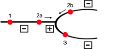
during

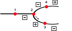
after

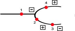
Figure 3.5. A description of a merge event. The nodal points (2a) and (2b) merge and become the nodal point (2). The signs of the nodal domains of $f^{(k)}$ are marked with squares.

However, a short while before this event, the neighborhood of this vertex was contained in a single nodal domain with a definite sign. The $k$-continuity of the solution implies that this is possible only if a short while before the event there was another nodal point in the vicinity of the vertex that has disappeared while merging with the nodal point at the vertex (see figure 3.5-before) . A similar reasoning shows that split events occur for odd $p$ values.

We have treated by now the possibility that the nodal point at the vertex had arrived from the lead. It might also happen that $f(k;\,\cdot)$ equals zero at a vertex of $\tilde{\Gamma}$ when $f(k;\,\cdot)$ vanishes on the lead which is connected to that vertex. For the real contra-phasal solution given in (3.26) this happens exactly at $\gamma\left(k\right)=\pi\mathbb{Z}$. This event would happen only on vertex number two for that solution (and on vertex number one for the reflected solution). These events do not change the number of nodal points on the graph, and therefore we do not need to keep track of them.

∎

Lemma 3.11.

Let $a,b,c$ be positive real numbers such that $\frac{b}{c}\notin\mathbb{Q}$ and $\frac{a}{b+c}\notin\mathbb{Q}$ and $\Gamma$, $\tilde{\Gamma}$ be the graphs described above. The number of nodal points on $\Gamma$ of a real contra-phasal solution on $\tilde{\Gamma}$ is increased by one at $k$ such that $k^{2}\in\sigma\left(\Gamma\right)$.

Proof.

When $k$ equals an eigenvalue of $\Gamma$, the solution restricted on $\Gamma$ equals an eigenfunction of $\Gamma$, i.e., either $f_{1}(k;\,a)=0$ or $f_{2}(k;\,a)=0$. A nodal point is therefore positioned on the boundary of $\Gamma$, and from lemma 3.9 we deduce that this nodal point moves towards the cycle, increasing by one the number of nodal points on $\Gamma$. It is only left to verify that there is no simultaneous split or merge events which further change the total number of nodal points. Namely, we show that $\left\{k_{p}^{*}\right\}$ and $\sigma\left(\Gamma\right)$ are disjoint sets. Assume the contrary: $k_{p}^{*}\in\sigma\left(\Gamma\right)$ for some $p$. By definition, $f_{j}(k_{p}^{*};\,0)=0$ for $j\in\left\{1,2\right\}$. Assume without loss of generality that $f_{1}(k_{p}^{*};\,0)=0$. Then, since $k_{p}^{*}\in\sigma\left(\Gamma\right)$ we also have that either $f_{1}(k_{p}^{*};\,a)=0$ or $f_{1}^{\prime}(k_{p}^{*};\,a)=0$. If $f_{1}(k_{p}^{*};\,a)=0$ then $k_{p}^{*}\in\frac{\pi}{a}\mathbb{Z}$ and applying lemma 3.10 gives $\frac{\pi}{2b+2c}\in\frac{\pi}{a}\mathbb{Z}$, which contradicts the incommensurability assumption. Otherwise, if $f_{1}^{\prime}(k_{p}^{*};\,a)=0$, we similarly obtain $\frac{\pi}{2b+2c}\in\frac{\pi}{2a}+\frac{\pi}{a}\mathbb{Z}$, and again get a contradiction.

∎

Lemma 3.12.

Let the set $\left\{k_{p}^{*}\right\}$, as defined in lemma 3.10, be the set of $k$ values at which merge and split events occur, and let $k_{0}^{*}=0$. Denote $d_{p}:=\left|\left\{k^{2}\in\sigma\left(\Gamma\right)\left|k_{p-1}^{\ast}<k<k_{p}^{\ast}\right.\right\}\right|$ , the number of eigenvalues of $\Gamma$ that occurred between two consequent merge/split events. Then

(3.29) $$d_{p}=\left\lfloor\frac{a}{b+c}p\right\rfloor-\left\lfloor\frac{a}{b+c}\left(p-1\right)\right\rfloor+1.$$

Proof.

The following two observations concern the set $D_{1}\left(k\right)\cup D_{2}\left(k\right)$, which gives the positions of the nodal points on the leads.

The spectrum of $\Gamma$ may be characterized as

(3.30) $$\sigma\left(\Gamma\right)=\left\{k^{2}\,\left|\,a\in D_{1}\left(k\right)\cup D{}_{2}\left(k\right)\right.\right\}.$$

The merge/split events happen at

(3.31) $$\left\{k_{p}^{*}\right\}=\left\{k\,\left|\,0\in D_{1}\left(k\right)\cup D_{2}\left(k\right)\right.\right\}.$$

We denote $Q\left(k\right):=\left(\left.0,a\right.\right]\cap\left\{D_{1}\left(k\right)\cup D_{2}\left(k\right)\right\}$ and describe how it changes with $k$. Lemma 3.9 implies that the values of $Q\left(k\right)$ continuously decrease with $k$. In addition, the first observation gives that $\left|Q\left(k\right)\right|$ increases at $k\in\sigma\left(\Gamma\right)$, when a nodal point enters $\Gamma$. The second observation shows that $\left|Q\left(k\right)\right|$ decreases by one at $k\in\left\{k_{p}^{*}\right\}$ , when a nodal point enters the cycle. It is therefore evident that during the interval $\left(\left.k_{p-1}^{*},k_{p}^{*}\right.\right],$ $\left|Q\left(k\right)\right|$ decreased a single time (at $k_{p}^{*}$), and the number of times it increased is given by $d_{p}$, the number of eigenvalues in this interval. We conclude that

(3.32) $$d_{p}=\left|Q\left(k_{p}^{*}\right)\right|-\left|Q\left(k_{p-1}^{*}\right)\right|+1.$$

It is easy to see that $D_{1}\left(k_{p}^{*}\right)\cup D_{2}\left(k_{p}^{*}\right)=\frac{\pi}{2k_{p}^{*}}\mathbb{Z}$, and therefore

$$\left|Q(k_{p}^{*})\right|=\left|\left(\left.0,a\right.\right]\cap\frac{\pi}{2k_{p}^{*}}\mathbb{Z}\right|=\left\lfloor\frac{2k_{p}^{\ast}a}{\pi}\right\rfloor.$$

Substituting $k_{p}^{*}=\frac{\pi}{2b+2c}p$ (lemma 3.10) and plugging this in (3.32) gives (3.29).

∎

We now have all the required information to obtain an expression for $\mu_{n}$, the number of nodal points on $\Gamma$ at $k=k_{n}$.

Proof.

[Proof of theorem 3.3]

In order to prove (3.18) we need to keep track of all the events which affect the number of nodal points on the graph. These include the eigenvalues of the original graph,$\left\{k_{n}\right\}$, and the merge/split events, $\left\{k_{p}^{*}\right\}$. Figure 3.6 shows a possible scenario for such a stream of events. In this figure, the value of $\mu_{n}-n$ is shown for each eigenvalue. The bounds on $\mu_{n}-n$ can be obtained from (1.10) with a slight modification due to the additional nodal point positioned on the Dirichlet vertex of the graph: 0$\leq\mu_{n}-n\leq 1$. The value of $\mu_{n}-n$ differs from $\mu_{n-1}-\left(n-1\right)$ if and only if a merge/split event occurred in between the corresponding eigenvalues. We therefore conclude that the value of $\mu_{n}-n$ depends on the parity of the number of merge/split events that occurred before $k_{n}$.

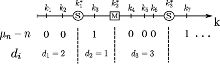
Figure 3.6. An example of a stream of events needed to keep track of the number of nodal points.

Namely,

$$\mu_{n}-n=\operatorname{mod}_{2}p,$$

where $p$ is an integer such that

$$k_{p}^{\ast}<k_{n}<k_{p+1}^{\ast}.$$

By the definition of $d_{p}$ (see lemma 3.12) this is equivalent to

$$\sum_{i=1}^{p}d_{i}<n\leq\sum_{i=1}^{p+1}d_{i},$$

which by (3.29) evaluates to

$$\left\lfloor\frac{a}{b+c}p\right\rfloor+p<n\leq\left\lfloor\frac{a}{b+c}\left(p+1\right)\right\rfloor+\left(p+1\right).$$

Since $n,\,p$ are integers and $\frac{a}{b+c}\notin\mathbb{Q}$,

$$\frac{a}{b+c}p+p<n\leq\frac{a}{b+c}\left(p+1\right)+\left(p+1\right).$$

Multiplying through by $\frac{b+c}{a+b+c}$ we get

$$p<\frac{b+c}{a+b+c}n<\left(p+1\right),$$

and conclude that

$$p=\left\lfloor\frac{b+c}{a+b+c}n\right\rfloor.$$

The number of nodal points on the graph is therefore given by

$$\mu_{n}=n+\operatorname{mod}_{2}\left(\left\lfloor\frac{b+c}{a+b+c}n\right\rfloor\right).$$

We now wish to turn this into a formula for the nodal count, $\nu_{n}$. The relation between $\mu_{n}$ and $\nu_{n}$ depends on whether the $n^{th}$ eigenfunction has nodal points on the loop as demonstrated in figure 3.7.

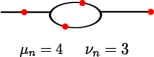
(a)     (b)

Figure 3.7. The two possible relations between the number of nodal points, $\mu_{n}$, and the number of nodal domains, $\nu_{n}$.

If it does have nodal points on the loop then $\nu_{n}=\mu_{n}-1$ (figure 3.7(b)), and in the case it does not, $\nu_{n}=\mu_{n}$ (figure 3.7(a)).
We therefore have that for the first $d_{1}=\left\lfloor\frac{a}{b+c}\right\rfloor+1$ eigenvalues (when there are still no nodal points on the loop) the nodal count is

$$\nu_{n}=n+\operatorname{mod}_{2}\left(\left\lfloor\frac{b+c}{a+b+c}n\right\rfloor\right)=n,$$

where the second equality is due to $n\leq\left\lfloor\frac{a}{b+c}\right\rfloor+1$. For the rest of the nodal count, $n>\left\lfloor\frac{a}{b+c}\right\rfloor+1$, we get

$$\nu_{n}=n-1+\operatorname{mod}_{2}\left(\left\lfloor\frac{b+c}{a+b+c}n\right\rfloor\right).$$

∎

4. The nodal count of graphs with disjoint cycles

4.1. Graphs with $\beta=1$: a dynamical approach

In this section we will discuss the nodal dynamics on a graph with one cycle (i.e. $\beta=1$) and a lead attached to a general position on the cycle, see figure 4.1. The discussion will not be formal, as we will prove the results by other methods in section 4.2.

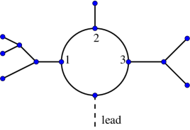
Figure 4.1. An example of a graph $\Gamma$ with $\beta=1$. We view it as a cycle with trees grafted upon it.

We have seen in section 3.1 that, as $k$ increases the nodal points (zeroes) travel along the lead in the direction of the graph. Consider the quantity $\delta_{n}=\mu_{n}-n+1$. This is the “surplus” of zeros due to the graph not being a tree. Bound (1.10) implies that $\delta_{n}$ can be equal to either $0$ or $1$. The change in this quantity from eigenvalue $k=k_{n-1}$ to eigenvalue $k=k_{n}$ can be attributed to the following three causes:

1. The increase in the index $n$ (the change in $d$ is $-1$).

2. A zero entering the graph from the lead. Upon entering, the zero can either merge (M) with a zero already present on the cycle or split (S) into two zeros.

3. A zero entering a tree. This zero can either split off a zero traveling on the cycle or it can be a result of two zeros from the cycle merging together.

Another notable event is a zero passing through a vertex where a tree is attached. We did not list it above since an event of this type does not affect the nodal count. Similarly, when a zero is traveling through the tree, we know (see [15, 17, 20]) that the number of zeros does not change.

As already explained in section 3.1, event (2) happens exactly once between each pair of eigenvalues $k_{n-1}$ and $k_{n}$, since an eigenvalue corresponds to the Neumann condition and the entrance event corresponds to the Dirichlet condition satisfied at the attachment point. If event (2) is a split, the contribution to $\delta$ is $+2$, otherwise it is $0$. However, if we consider the total contribution of events (1) and (2), we get $+1$ from a split and $-1$ from a merge. This is the same as a contribution of a type (3) event, when the split results in $+1$ (number of zeros on the cycle stays the same but another zero appears on a tree) and the merge in $-1$ (the number of zeros on the cycle reduces by $2$, while one zero enters a tree).

The first eigenfunction has constant sign, so $\delta_{1}=0$ and no events happen until $k=k_{1}$. Since the contribution of type (1) is now absorbed in the contributions of type (2), the value of $\delta_{n}$ is the total number of splits minus the total number of merges up to $k=k_{n}$. On the other hand, $\delta_{n}$ is restricted by the nodal bound to be either $1$ or $0$, therefore it is equal to the parity of the total number of S/M events.

There are exactly $n-1$ events of type (2) happening until $k=k_{n}$. To count the number of events of type (3), we consider an auxiliary graph $\Gamma_{\emptyset}$, obtained from $\Gamma$ by removing all edges belonging to the cycle and imposing Dirichlet conditions on the points where the trees were connected to the cycle. The graph $\Gamma_{\emptyset}$ is a collection of trees that were grafted on the cycle. Since a zero entering a tree signals that the Dirichlet condition is satisfied on the tree, the corresponding value of $k$ is in fact an eigenvalue of $\Gamma_{\emptyset}$. And the number of events of type (3) is thus equal to the number of eigenvalues of $\Gamma_{\emptyset}$ that are smaller than $k_{n}$. To summarize,

$$\delta_{n}=\operatorname{mod}_{2}(n-1+N_{\emptyset}(k_{n})),$$

where $N_{\emptyset}(k_{n})$ is the spectral counting function of the graph $\Gamma_{\emptyset}$. Thus we can fully predict the nodal count using the spectra of two graphs, $\Gamma$ and $\Gamma_{\emptyset}$. The discussion above captures the dynamics of the zeros, but it is relatively difficult to formalize. Instead we will prove the formula for $\mu_{n}$ by other methods, which, although not very pictorial, allow us to extend the argument to the case of non-zero potential $V(x)$.

4.2. Graphs with $\beta=1$: a formal proof

In this section we prove the formula that was informally derived in section 4.1.

Theorem 4.1.

Consider the Schrödinger operator (1.2) on a connected graph with a single cycle. Let the $n$-th eigenvalue be simple and the corresponding eigenfunction be non-zero on the vertices. Then

(4.1) $$\mu_{n}=n-1+\operatorname{mod}_{2}\left(n-1+N_{\emptyset}(\lambda_{n})\right),$$

where $N_{\emptyset}$ is the spectral counting function of the disconnected graph obtained by removing the cycle and putting Dirichlet conditions on the new vertices.

Proof.

From the nodal bound for graphs with one cycle (i.e. with $\beta=1$) we know that $\mu_{n}$ is equal to $n-1$ or $n$. The first step of the proof is to observe that the number of zeros on the edges that do not belong to the cycle is equal to $N_{\emptyset}(\lambda_{n})$. We will prove this statement below. Then $\mu_{n}-N_{\emptyset}(\lambda_{n})$ is the number of zeros on the cycle, and has to be even, as explained in section 1.2.

First, assume that $\mu_{n}=n$. Then, the quantity

$$\mu_{n}-1-N_{\emptyset}(\lambda_{n})=n-1-N_{\emptyset}(\lambda_{n})$$

is odd and therefore

$$\operatorname{mod}_{2}\left(n-1+N_{\emptyset}(\lambda_{n})\right)=\operatorname{mod}_{2}\left(n-1-N_{\emptyset}(\lambda_{n})\right)=1,$$

where we used the fact that

$$\operatorname{mod}_{2}(a+b)=\operatorname{mod}_{2}(a-b)$$

for any integer $a$ and $b$. Thus the right-hand side of equation (4.1) evaluates to $n$ which is the right answer.

If $\mu_{n}$ is not equal to $n$, then it is equal to $n-1$ and we have

$$\operatorname{mod}_{2}\left(n-1+N_{\emptyset}(\lambda_{n})\right)=\operatorname{mod}_{2}\left(\mu_{n}-N_{\emptyset}(\lambda_{n})\right)=0,$$

since $\mu_{n}-N_{\emptyset}(\lambda_{n})$ is even. Thus equation (4.1) still holds.

Now we prove that $N_{\emptyset}(\lambda_{n})$ is indeed the number of zeros on the subtrees of the graph. To shorten the formulas we introduce the following notation. We denote the $n$-th eigenvalue by $\Lambda$ and the corresponding eigenfunction by $F$. Break up the original graph into the cycle and the trees $T_{j}$. For each tree $T_{j}$ we choose as a root the vertex that was its contact point with the cycle. We can ensure that each root has degree 1: if necessary we can split trees that share a root. On each tree the vertex conditions are inherited from the graph, but we still need to specify the conditions on the root. We will consider two versions of each tree. The first, $T_{j,F}$ has the condition on the root $r$ chosen to be satisfied by the function $F$, restricted to the tree. That is we chose the constant $\alpha$ in the $\delta$-type condition to be $\alpha=F^{\prime}(r)/F(r)$. The second version of the tree, denoted $T_{j,\infty}$, has the Dirichlet condition on the root.

Denote by $T_{\infty}$, the disjoint union of the graphs $T_{j,\infty}$. We observe that

$$N_{\emptyset}(\lambda)=N_{T_{\infty}}(\lambda)=\sum_{j}N_{T_{j,\infty}}(\lambda).$$

Thus we only need to prove that $N_{T_{j,\infty}}(\Lambda)$ gives the number of zeros of $F$ on the subtree $T_{j,\infty}$. Since, by construction, the restriction of $F$ is an eigenfunction of $T_{j,F}$ with the eigenvalue $\Lambda$, we have $\Lambda=\lambda_{m}(T_{j,F})$ for some $m$. By the strict interlacing, theorem A.1,

$$\lambda_{m-1}(T_{j,\infty})<\lambda_{m}(T_{j,F})<\lambda_{m}(T_{j,\infty}),$$

and, therefore, $N_{T_{j,\infty}}(\Lambda)=m-1$. On the other hand, the nodal count on trees, equation (1.10), gives $\mu_{m}(T_{j,\infty})=m-1$. This concludes the proof. ∎

4.3. Number of zeros on a graph with disjoint cycles

In fact, the formula of the previous section can be extended to $\beta>1$ as long as the cycles do not share any vertices.

Theorem 4.2.

For a connected graph containing $\beta$ disjoint cycles, let the $n$-th eigenvalue be simple and the corresponding eigenfunction be non-zero on the vertices. Then

$$\mu_{n}=n-1+\sum_{j=1}^{\beta}\operatorname{mod}_{2}\left(n-1+N_{j,\emptyset}(\lambda_{n})\right),$$

where $N_{j,\emptyset}$ is the spectral counting function of the disconnected graph obtained by removing the $j$-th cycle and putting Dirichlet conditions on the new vertices.

Proof.

Denote the $n$-th eigenvalue by $\Lambda$ and the corresponding eigenfunction by $F$. Choose an arbitrary cycle and let $e_{1}$, …, $e_{k}$ be the edges incident to it. Since the cycles are disjoint, these edges do not belong to any cycle. Choose points $c_{1}$, …, $c_{k}$, one on each edge, so that the function $F$ is non-zero at these points. If the graph is cut at these points, we obtain $k+1$ disjoint subgraphs, $\Gamma_{j}$, $j=0,\ldots,k$ (the $0$-th subgraph contains the chosen cycle), see figure 4.2.

Figure 4.2. An example of a graph with 4 disjoint cycles. In part (a), the middle cycle is chosen and the cut-points are labeled. In part (b) the graph is split up into subgraphs. The central part $\Gamma_{0}$ contains exactly one cycle, while the other parts can contain more or fewer.

Define

$$\alpha_{c_{j}}=\frac{F^{\prime}(c_{j})}{F(c_{j})},$$

where the derivative is taken away from the chosen loop. We impose $\delta$-type conditions on the newly formed vertices. The vertex $c_{j}$ belonging to $\Gamma_{j}$ will get the condition with coefficient $\alpha_{c_{j}}$ and its counterpart belonging to the subgraph $\Gamma_{0}$ will get the condition with coefficient $-\alpha_{c_{j}}$. This way, the appropriately cut function $F$ is still an eigenfunction on all $k+1$ subgraphs and $\Lambda$ is the corresponding eigenvalue. This allows us to define $m_{j}$ by

$$\Lambda=\lambda_{m_{j}}(\Gamma_{j}).$$

Lemma 4.3.

The numbers $m_{j}$ are well-defined and satisfy

(4.2) $$n-1=\sum_{j=0}^{k}(m_{j}-1).$$

Proof of the lemma.

Let $\Gamma_{c}$ denote the disjoint union of the graphs $\Gamma_{j}$, $j=0,\ldots,k$. First of all, we apply theorem A.2 $k$ times (for $k$ cuts) to obtain inequalities

$$\lambda_{n-1}(\Gamma_{c})\leq\lambda_{n-1}(\Gamma)\qquad\mbox{and}\qquad\lambda_{n+1}(\Gamma)\leq\lambda_{n+k+1}(\Gamma_{c})$$

On the other hand, simplicity of the eigenvalue $\lambda_{n}(\Gamma)=\Lambda$ means that $\lambda_{n-1}(\Gamma)<\Lambda<\lambda_{n+1}(\Gamma)$ and therefore

(4.3) $$\lambda_{n-1}(\Gamma_{c})<\Lambda<\lambda_{n+k+1}(\Gamma_{c}).$$

Finally, out of $F$ we can form at least $k+1$ linearly independent eigenfunctions of the graph $\Gamma_{c}$: functions that are restrictions of $F$ on one of the parts $\Gamma_{j}$ and identically zero on all the others. All these eigenfunctions have eigenvalue $\Lambda$. Combining this observation with inequality (4.3) we conclude that $\Lambda$ has degeneracy exactly $k+1$ in the spectrum of $\Gamma_{c}$ and therefore is a simple eigenvalue of every part $\Gamma_{j}$. Thus the numbers $m_{j}$ are well-defined.

Finally, since the spectrum of $\Gamma_{c}$ is the superposition of spectra of $\Gamma_{j}$, equation (4.2) is equivalent to the statement “there are $n-1$ eigenvalues of $\Gamma_{c}$ that are strictly less than $\Lambda$”, which is also obvious from inequality (4.3) and the fact that $\lambda_{n}(\Gamma_{c})=\Lambda$. ∎

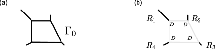
Figure 4.3. The subgraph $\Gamma_{0}$ and the graph $R$ obtained after removing the cycle (it appears shaded on part (b) of the figure). The graph $R$ is a disjoint union of four subgraphs $R_{j}$.

We now want to use theorem 4.1 to find the number of zeros of the function $F$ on the graph $\Gamma_{0}$. Let $R$ be the graph obtained from $\Gamma_{0}$ by removing the cycle and imposing Dirichlet conditions on the new vertices. This graph is a disjoint union of the graphs $R_{j}$, $j=1,\ldots,k$, see Fig. 4.3 Therefore, we have

(4.4) $$N_{R}(\Lambda)=\sum_{j=1}^{k}N_{R_{j}}(\Lambda).$$

According to theorem 4.1 the number of zeros of $F$ on the subgraph $\Gamma_{0}$ is

$$\mu(\Lambda,\Gamma_{0})=m_{0}-1+\operatorname{mod}_{2}\left(m_{0}-1+N_{R}(\Lambda)\right).$$

Extracting $m_{0}-1$ from equation (4.2) and using equation (4.4) we get

(4.5) $$\mu(\Lambda,\Gamma_{0})=m_{0}-1+\operatorname{mod}_{2}\left(n-1+\sum_{j=1}^{k}\left(m_{j}-1+N_{R_{j}}(\Lambda)\right)\right),$$

where we used

$$\operatorname{mod}_{2}(a+b)=\operatorname{mod}_{2}(a-b)$$

for integer $a$ and $b$ to change some signs. Define now the graph $G$ by removing the chosen cycle from the original graph $\Gamma$ and imposing the Dirichlet conditions on the new vertices. Similarly to the graph $R$, the graph $G$ is a disjoint union of $k$ subgraphs $G_{j}$, see Fig. 4.4, and

(4.6) $$N_{G}(\Lambda)=\sum_{j=1}^{k}N_{G_{j}}(\Lambda).$$

If we were to cut the graph $G_{j}$ at the point $c_{j}$ the two parts would be exactly $\Gamma_{j}$ and $R_{j}$. This suggests the following lemma.

Figure 4.4. The original graph $\Gamma$ and the graph $G$ obtained by removing the chosen cycle. The graph $G$ is a disjoint union of graphs $G_{j}$.

Lemma 4.4.

For every $j=1,\ldots,k$,

(4.7) $$N_{G_{j}}(\Lambda)=m_{j}-1+N_{R_{j}}(\Lambda).$$

Proof of the lemma.

First we observe that $\Lambda$ belongs to the spectrum of the graph $\Gamma_{j}$ and does not belong to the spectrum of $R_{j}$ or $G_{j}$. This can be shown by the strict interlacing, theorem A.1, applied to the graph $\Gamma$ (corresp. $G_{0}$) by changing the condition from Neumann to Dirichlet at the vertex where $G_{j}$ (corresp. $R_{j}$) was connected to the cycle.

Denote by $G_{j,c}$ the disjoint union of the graphs $\Gamma_{j}$ and $R_{j}$. Let integer $q$ be such that

$$\Lambda=\lambda_{q}(G_{j,c}).$$

Since $\Lambda=\lambda_{m_{j}}(\Gamma_{j})$, we have that $q=m_{j}+N_{R_{j}}(\Lambda)$. On the other hand, by theorem A.2,

$$\lambda_{q-1}(G_{j})<\Lambda=\lambda_{q}(G_{j,c})<\lambda_{q}(G_{j})$$

Therefore, $N_{G_{j}}(\Lambda)=q-1$ which concludes the proof. ∎

Combining equations (4.6) and (4.7) with formula (4.5) we arrive to

(4.8) $$\mu(\Lambda,\Gamma_{0})=m_{0}-1+\operatorname{mod}_{2}\left(n-1+N_{G}(\Lambda)\right).$$

We should also note that $N_{G}=N_{j,\emptyset}$, where $j$ is the number of the cycle that was chosen.

Since we chose an arbitrary cycle, equation (4.8) is valid for every cycle. The conclusion of the theorem is just the sum of equations (4.8) over all cycles with an application of the analogue of equation (4.2). ∎

5. A discussion

5.1. An approximate derivation of an exact nodal count formula

We will now present an alternative way to get the nodal points count formula (3.18) of the graph given in figure 5.1(a). The derivation is most appealing, but involves an approximation that cannot be justified. We present it here because it makes use of an idea which has been used in other contexts. Also we find that an unjustifiable approximation that reproduces the exact nodal count formula carries information about the graph in its own right.

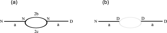
Figure 5.1. (a) The quantum graph whose nodal count we compute. (b) The same graph with its cycle removed (appears shaded).

We start by rewriting the formula (4.1) with a slight modification, due to the nodal point which is positioned on the Dirichlet boundary vertex of the graph:

$$\mu_{n}=n+\operatorname{mod}_{2}\left(n+N_{\emptyset}(k_{n})\right).$$

The spectra of the two edges which appear in figure 5.1(b) are $\left\{\frac{\pi}{a}n\right\}_{n\in\mathbb{N}}$ and $\left\{\frac{\pi}{a}\left(n+\frac{1}{2}\right)\right\}_{n\in\mathbb{N}}$. Their spectral counting function is therefore

$$N_{\emptyset}(k)=\left\lfloor\frac{ka}{\pi}\right\rfloor+\left\lfloor\frac{ka}{\pi}+\frac{1}{2}\right\rfloor.$$

Plugging it above and using the identities $\operatorname{mod}_{2}\left(\left\lfloor x\right\rfloor+\left\lfloor x+\frac{1}{2}\right\rfloor\right)=\operatorname{mod}_{2}\left(\left\lfloor 2x\right\rfloor\right)$ and $\operatorname{mod}_{2}\left(x+y\right)=\operatorname{mod}_{2}\left(x-y\right)$ we obtain

$$\mu_{n}=n+\operatorname{mod}_{2}\left(n-\left\lfloor\frac{2k_{n}a}{\pi}\right\rfloor\right).$$

We can get an approximate expression for $k_{n}$ from the Weyl term of the spectral counting function of the graph,

$$N\left(k\right)\approx\frac{2(a+b+c)}{\pi}k,$$

by its inversion, i.e.,

$$k_{n}\approx\frac{\pi}{2(a+b+c)}n.$$

Using this approximation gives

$$\mu_{n} \approx n+\operatorname{mod}_{2}\left(n-\left\lfloor\frac{a}{a+b+c}n\right\rfloor\right)$$

$$=n+\operatorname{mod}_{2}\left(\left\lfloor\frac{b+c}{a+b+c}n\right\rfloor\right),$$

which is the exact result, (3.18).

One should note that the last step of the derivation, which involves an approximation of $k_{n}$ by inverting the Weyl term, cannot be justified. Moreover, the floor function is a discontinuous function and it is therefore expected that an approximation of its argument would lead to a completely wrong result for some portion of the sequence.

From the exactness of the final result, we conclude the following property of the spectrum

$$N_{\emptyset}(k_{n})=\operatorname{mod}_{2}\left(\left\lfloor\frac{2a}{\pi}\,k_{n}\right\rfloor\right)=\operatorname{mod}_{2}\left(\left\lfloor\frac{2a}{\pi}\,\frac{\pi}{2(a+b+c)}n\right\rfloor\right).$$

Numeric examination reveals that the equality hold for the arguments of the $\operatorname{mod}_{2}$ as well, namely

(5.1) $$\left\lfloor\frac{2a}{\pi}\,k_{n}\right\rfloor=\left\lfloor\frac{2a}{\pi}\,\frac{\pi}{2(a+b+c)}n\right\rfloor.$$

The above relation connects the spectrum and the lengths of the graph’s edges. Having such a relation for our graph makes $N_{\emptyset}(k_{n})$ expressible in terms of the parameters $a,b,c$ and enables to turn the nodal count formula, (4.1), into a formula which contains geometric properties of the graph, rather than spectral ones. In short, the special nodal count formula is a direct consequence of a purely spectral identity - a connection between the graph’s spectrum and the spectral counting function of its subgraphs.

The novelty of this result makes one wonder to what extent it can be generalized to other graphs. Even if such an exact result is not reproduced, one may still use approximations of the type above and try to estimate the errors caused by them.

5.2. Periodic orbits expansions

Wishing to express the nodal count formula (3.18) as a periodic orbits expansion, we notice that $\operatorname{mod}_{2}\left(\left\lfloor x\right\rfloor\right)$ is an odd periodic function (of period 2), whose Fourier transform is:

$$\operatorname{mod}_{2}\left(\left\lfloor x\right\rfloor\right)=\frac{1}{2}-\sum_{k=0}^{\infty}\frac{2}{(2k+1)\pi}\sin\left(\left(2k+1\right)\pi x\right).$$

Denoting $\alpha:=\frac{b+c}{a+b+c}$, the normalized length of the loop, we can rewrite (3.18) as following:

$$\mu_{n}=n+\frac{1}{2}-\sum_{k=0}^{\infty}\frac{2}{(2k+1)\pi}\sin\left(\left(2k+1\right)\pi\alpha n\right).$$

We therefore get that the nodal points sequence is expressed in terms of lengths of periodic orbits on the graph. One should note that the only periodic orbits that appear are odd repetitions of the graph’s cycle. They appear with harmonically decaying amplitudes. This causes to seek for a more direct derivation of the periodic orbits expansion which may also explain the meaning of the amplitudes and the absence of other periodic orbits. Furthermore, the formula (4.1), which holds for any graph with a single cycle, may also be turned into an expansion of a similar type. We recall that for quantum graphs there exist an exact periodic expansion for the spectral counting function. Therefore, the spectral counting function of the subgraph, $N_{\emptyset}(k_{n})$, can be expanded and plugged in formula (4.1). This would yield an expansion which still involves the spectral information, $\left\{k_{n}\right\}$. Having an approximate inversion of the spectral counting function of the whole graph then enables to further get a periodic orbits formula which involves only geometric properties of the graph. Such spectral inversion attempts were recently carried out with a high degree of success [10, 42]. It is therefore evident that the obtained result leads to a wide field of further questions and open research possibilities.

6. acknowledgments

It is a pleasure to acknowledge Sven Gnutzmann for fruitful discussions about the scattering matrix properties. We are grateful to Peter Kuchment for suggesting to extend Theorem 4.1 to what is now Theorem 4.2. We also wish to thank Amit Godel for the careful examination of the proof of theorem 3.3. The work was supported by the Minerva Center for Nonlinear Physics, the Einstein (Minerva) Center at the Weizmann Institute and the Wales Institute of Mathematical and Computational Sciences) (WIMCS). Grants from EPSRC (grant EP/G021287), ISF (grant 166/09), BSF (grant 2006065) and NSF (DMS-0604859 and DMS-0907968) are acknowledged.

Appendix A Interlacing theorems for quantum graphs

Eigenvalue interlacing (or bracketing) is a powerful tool in spectral theory. In particular, in the graph setting, it allows to estimate eigenvalue of a given graph via the eigenvalues of its subgraphs, which may be easier to calculate. Here we quote the theorems that are used in the proofs of the formulas of the present manuscript. The theorems are quoted in the form they appear in [35].

The first theorem deals with choosing a vertex on the graph $\Gamma$ and changing the parameter $\alpha_{v}$ of the extended $\delta$-type condition at $v$ (see equation (1.4)). We remind the reader that $\alpha_{v}=\infty$ corresponds to the Dirichlet condition at the vertex which essentially disconnects the edges meeting at the vertex.

Theorem A.1 (Interlacing when changing a parameter).

Let $\Gamma_{\alpha^{\prime}}$ be the graph obtained from the graph $\Gamma_{\alpha}$ by changing the coefficient of the condition at vertex $v$ from $\alpha$ to $\alpha^{\prime}$. If $-\infty<\alpha<\alpha^{\prime}\leq\infty$, then

(A.1) $$\lambda_{n}(\Gamma_{\alpha})\leq\lambda_{n}(\Gamma_{\alpha^{\prime}})\leq\lambda_{n+1}(\Gamma_{\alpha}).$$

If the $n$-th eigenvalue of $\Gamma_{\alpha^{\prime}}$ is simple and the corresponding eigenfunction is nonzero on the vertices, the inequalities are strict.

The second theorem deals with the situation when the graph $\Gamma^{\prime}$ is obtained from $\Gamma$ by gluing two vertices together, or, equivalently, $\Gamma$ is obtained by cutting the graph $\Gamma^{\prime}$ at a vertex or at a point on an edge. When gluing the vertices together, their respective parameters $\alpha_{v_{0}}$ and $\alpha_{v_{1}}$ get added.

Theorem A.2 (Interlacing when gluing the vertices).

Let $\Gamma$ be a compact (not necessarily connected) graph. Let $v_{0}$ and $v_{1}$ be vertices of the graph $\Gamma$ endowed with the $\delta$-type conditions with the parameters $\alpha_{0}$ and $\alpha_{1}$ (see definition 1.1). Arbitrary self-adjoint conditions are allowed at all other vertices of $\Gamma$.

Let $\Gamma^{\prime}$ be the graph obtained from $\Gamma$ by gluing the vertices $v_{0}$ and $v_{1}$ together into a single vertex $v$, so that $\mathcal{E}_{v}=\mathcal{E}_{v_{0}}\cup\mathcal{E}_{v_{1}}$, and endowed with the $\delta$-type condition with the parameter $\alpha_{v}=\alpha_{0}+\alpha_{1}$.

Then the eigenvalues of the two graphs satisfy the inequalities

(A.2) $$\lambda_{n}(\Gamma)\leq\lambda_{n}(\Gamma^{\prime})\leq\lambda_{n+1}(\Gamma).$$

In addition, if $\lambda_{n}(\Gamma^{\prime})$ is simple and the corresponding eigenfunction is nonzero on vertices and not an eigenfunction of $\Gamma$, the inequalities are strict.

An intuitive explanation for the above result is that by gluing vertices we impose an additional restriction: the continuity condition. This additional restriction pushes the spectrum up.

References

- [1] P. Kuchment, “Graph models for waves in thin structures,” Waves Random Media, vol. 12, no. 4, pp. R1–R24, 2002.
- [2] S. Gnutzmann and U. Smilansky, “Quantum graphs: Applications to quantum chaos and universal spectral statistics,” Adv. Phys., vol. 55, no. 5–6, pp. 527–625, 2006.
- [3] G. Berkolaiko, R. Carlson, S. Fulling, and P. Kuchment, eds., Quantum graphs and their applications, vol. 415 of Contemp. Math., (Providence, RI), Amer. Math. Soc., 2006.
- [4] P. Exner, J. P. Keating, P. Kuchment, T. Sunada, and A. Teplyaev, eds., Analysis on graphs and its applications, vol. 77 of Proc. Sympos. Pure Math., (Providence, RI), Amer. Math. Soc., 2008.
- [5] R. Courant and D. Hilbert, Methods of mathematical physics. Vol. I. Interscience Publishers, Inc., New York, N.Y., 1953.
- [6] Å. Pleijel, “Remarks on Courant’s nodal line theorem,” Comm. Pure Appl. Math., vol. 9, pp. 543–550, 1956.
- [7] G. Blum, S. Gnutzmann, and U. Smilansky, “Nodal domains statistics: A criterion for quantum chaos,” Physical Review Letters, vol. 88, p. 114101, Mar. 2002.
- [8] E. Bogomolny and C. Schmit, “Percolation Model for Nodal Domains of Chaotic Wave Functions,” Physical Review Letters, vol. 88, p. 114102, Mar. 2002.
- [9] F. Nazarov and M. Sodin, “On the number of nodal domains of random spherical harmonics,” arXiv:0706.2409v1 [math-ph], June 2007.
- [10] S. Gnutzmann, P. D. Karageorge, and U. Smilansky, “Can one count the shape of a drum?,” Physical Review Letters, vol. 97, no. 9, p. 090201, 2006.
- [11] S. Gnutzmann, U. Smilansky, and N. Sondergaard, “Resolving isospectral ’drums’ by counting nodal domains,” Journal of Physics A Mathematical General, vol. 38, pp. 8921–8933, Oct. 2005.
- [12] D. K. J. Brüning and C. Puhle, “Comment on “resolving isospectral ‘drums’ by counting nodal domains",” J. Phys. A: Math. Theor., vol. 40, pp. 15143–15147, 2007.
- [13] P. D. Karageorge and U. Smilansky, “Counting nodal domains on surfaces of revolution,” J. Phys. A: Math. Theor., vol. 41, p. 205102 (26pp), 2008.
- [14] O. Al-Obeid, “On the number of the constant sign zones of the eigenfunctions of a dirichlet problem on a network (graph),” tech. rep., Voronezh: Voronezh State University, 1992. in Russian, deposited in VINITI 13.04.93, N 938 – B 93. – 8 p.
- [15] Y. V. Pokornyĭ, V. L. Pryadiev, and A. Al′-Obeĭd, “On the oscillation of the spectrum of a boundary value problem on a graph,” Mat. Zametki, vol. 60, no. 3, pp. 468–470, 1996.
- [16] Y. V. Pokornyĭ and V. L. Pryadiev, “Some problems in the qualitative Sturm-Liouville theory on a spatial network,” Uspekhi Mat. Nauk, vol. 59, no. 3(357), pp. 115–150, 2004.
- [17] P. Schapotschnikow, “Eigenvalue and nodal properties on quantum graph trees,” Waves Random Complex Media, vol. 16, no. 3, pp. 167–178, 2006.
- [18] S. Gnutzmann, U. Smilansky, and J. Weber, “Nodal counting on quantum graphs,” Waves Random Media, vol. 14, no. 1, pp. S61–S73, 2004. Special section on quantum graphs.
- [19] E. B. Davies, G. M. L. Gladwell, J. Leydold, and P. F. Stadler, “Discrete nodal domain theorems,” Linear Algebra Appl., vol. 336, pp. 51–60, 2001.
- [20] G. Berkolaiko, “A lower bound for nodal count on discrete and metric graphs,” Comm. Math. Phys., vol. 278, no. 3, pp. 803–819, 2008.
- [21] R. Band, T. Shapira, and U. Smilansky, “Nodal domains on isospectral quantum graphs: the resolution of isospectrality?,” Journal of Physics A Mathematical General, vol. 39, pp. 13999–14014, 2006.
- [22] R. Band, I. Oren, and U. Smilansky, “Nodal domains on graphs—how to count them and why?,” in Analysis on graphs and its applications, vol. 77 of Proc. Sympos. Pure Math., pp. 5–27, Providence, RI: Amer. Math. Soc., 2008.
- [23] T. Kottos and U. Smilansky, “Chaotic scattering on graphs,” Phys. Rev. Lett., vol. 85, no. 5, pp. 968–971, 2000.
- [24] T. Kottos and U. Smilansky, “Quantum graphs: a simple model for chaotic scattering,” J. Phys. A, vol. 36, no. 12, pp. 3501–3524, 2003. Random matrix theory.
- [25] E. B. Davies and A. Pushnitski, “Non-Weyl Resonance Asymptotics for Quantum Graphs,” ArXiv e-prints, Mar. 2010.
- [26] E. B. Davies, P. Exner, and J. Lipovsky, “Non-Weyl asymptotics for quantum graphs with general coupling conditions,” ArXiv e-prints, Apr. 2010.
- [27] P. Exner and J. Lipovský, “Resonances from perturbations of quantum graphs with rationally related edges,” Journal of Physics A Mathematical General, vol. 43, pp. 105301–+, Mar. 2010.
- [28] D. E. Edmunds and W. D. Evans, Spectral theory and differential operators. Oxford Mathematical Monographs, New York: The Clarendon Press Oxford University Press, 1987. Oxford Science Publications.
- [29] V. Kostrykin and R. Schrader, “Kirchhoff’s rule for quantum wires,” J. Phys. A, vol. 32, no. 4, pp. 595–630, 1999.
- [30] M. Harmer, “Hermitian symplectic geometry and extension theory,” J. Phys. A, vol. 33, no. 50, pp. 9193–9203, 2000.
- [31] P. Kuchment, “Quantum graphs. I. Some basic structures,” Waves Random Media, vol. 14, no. 1, pp. S107–S128, 2004. Special section on quantum graphs.
- [32] C. Sturm, “Mémoire sur les équations différentielles linéaires du second ordre,” J. Math. Pures Appl., vol. 1, pp. 106–186, 1836.
- [33] C. Sturm, “Mémoire sur une classe d’équations à différences partielles,” J. Math. Pures Appl., vol. 1, pp. 373–444, 1836.
- [34] D. Hinton, “Sturm’s 1836 oscillation results: evolution of the theory,” in Sturm-Liouville theory, pp. 1–27, Basel: Birkhäuser, 2005.
- [35] G. Berkolaiko and P. Kuchment, “Dependence of the spectrum of a quantum graph on vertex conditions and edge lengths.” arXiv:1008.0369, 2010.
- [36] T. Kottos and U. Smilansky, “Periodic orbit theory and spectral statistics for quantum graphs,” Ann. Physics, vol. 274, no. 1, pp. 76–124, 1999.
- [37] T. Kottos and H. Schanz, “Statistical properties of resonance widths for open quantum graphs,” Waves Random Media, vol. 14, no. 1, pp. S91–S105, 2004. Special section on quantum graphs.
- [38] J. Bolte and S. Endres, “Trace formulae for quantum graphs,” in Analysis on graphs and its applications, vol. 77 of Proc. Sympos. Pure Math., pp. 247–259, Providence, RI: Amer. Math. Soc., 2008.
- [39] L. Friedlander, “Genericity of simple eigenvalues for a metric graph,” Israel J. Math., vol. 146, pp. 149–156, 2005.
- [40] R. Band, O. Parzanchevski, and G. Ben-Shach, “The isospectral fruits of representation theory: Quantum graphs and drums,” J. Phys. A: Math. Theor., vol. 42, p. 175202, 2009.
- [41] R. Band, I. Oren, and U. Smilansky, “Nodal domains on graphs - how to count them and why?,” in Analysis on Graphs and its Applications, Proc. Symp. Pure. Math., pp. 5–28, AMS, 2008.
- [42] R. Blümel, Y. Dabaghian, and R. V. Jensen, “Explicitly solvable cases of one-dimensional quantum chaos,” Phys. Rev. Lett., vol. 88, p. 044101, Jan 2002.