Observational upper limits on the gravitational wave production of core collapse supernovae

Abstract

The upper limit on the energy density of a stochastic gravitational wave (GW) background obtained from the two-year science run (S5) of the Laser Interferometer Gravitational-wave Observatory (LIGO) is used to constrain the average GW production of core collapse supernovae (ccSNe). We assume that the ccSNe rate tracks the star formation history of the universe and show that the stochastic background energy density depends only weakly on the assumed average source spectrum. Using the ccSNe rate for $z\leq 10$, we scale the generic source spectrum to obtain an observation-based upper limit on the average GW emission. We show that the mean energy emitted in GWs can be constrained within $<(0.49-1.98)\hskip 2.84526ptM_{\odot}c^{2}$ depending on the average source spectrum. While these results are higher than the total available gravitational energy in a core collapse event, second and third generation GW detectors will enable tighter constraints to be set on the GW emission from such systems.

1 Introduction

Core collapse supernovae (ccSNe), neutron star (NS) births and black hole (BH) births have long been considered to be likely observational sources of gravitational waves (GWs). For many decades effort has gone into estimating the GW emission from such sources (see, e.g., Thorne 1987; Houser et al. 1994; Fryer et al. 2001; Baiotti et al. 2007). Approaches to the problem have included numerical modelling of ccSNe, study of normal modes in newly born NSs and BHs, and constraints based on the observed asymmetry of supernovae or NS kick velocities.

Early estimates for the GW production were $\sim$ a few percent of rest mass energy, and estimates of gravitational energy loss from bar mode instabilities in newly born NSs were also quite high. Recent ccSNe modeling gives much lower predictions of GW production. For core collapse leading to NS births, predictions for the total energy emitted in GWs have been in the range $\sim(10^{-12}-10^{-4})\hskip 2.84526ptM_{\odot}c^{2}$ (Ott, 2009). For BH births the conversion efficiency to GWs is of the order $\sim(10^{-7}-10^{-6})M_{\odot}c^{2}$ (Baiotti & Rezzolla, 2006). However, there is significant uncertainty in supernova modelling due to the incomplete understanding of the explosion mechanism and the complexity of the physics involved (see Ott (2009) for a comprehensive review).

It is generally agreed that the frequency of GW emission from the birth of stellar mass collapsed objects is in the range 50Hz to a few kHz (Müller, 1997; Dimmelmeier et al., 2002, 2008). On the other hand, predictions of GW waveforms from ccSNe depend strongly on the considered emission mechanism. We argue below that a generic broad Gaussian spectrum provides a suitable average source spectrum.

Studies of the star formation rate in the universe allow estimation of the birth rate of collapsed objects. This rate is $\sim 10^{2}\hskip 2.84526pt\rm{s}^{-1}$ as discussed below. This is sufficient to create a quasi-continuous stochastic gravitational wave background (SGWB) of astrophysical origin in the above frequency band, with significant smearing to lower frequencies due to redshift. The amplitude of this background depends overwhelmingly on the average GW production for the individual events that combine to create this background.

The first generation interferometric GW detectors, including LIGO (Abadie et al., 2010d), Virgo (Accadia et al., 2010), GEO600 (Grote et al., 2010) and TAMA300 (Arai et al., 2008) have operated for long periods at astrophysically significant sensitivity (Kawamura, 2010). They have enabled constraints to be placed on various sources of GWs, e.g., pulsars (Abbott et al., 2008a, 2010a), deformed NSs (Abadie et al., 2010c), gamma ray bursts (Abbott et al., 2008c, 2010b) and coalescing compact binaries (Abbott et al., 2009a). In particular, blind all-sky burst searches with LIGO, Virgo and GEO600 detectors set limits for nearby ccSNe that exploded during data taking (Abadie et al., 2010a). In this regard, LIGO and Virgo are currently developing searches for GW bursts triggered by gamma ray, optical, radio and neutrino transients.

Recently the LIGO Scientific Collaboration and Virgo Collaboration used data from a two-year science run (S5) to constrain the energy density of SGWB in the frequency band $(41.5-169.25)\hskip 2.84526pt\rm{Hz}$ to be $<6.9\times 10^{-6}$ (denoted as LV limit; Abbott et al., 2009b). This was interpreted in terms of a cosmological background due to the big bang and exceeds the previous indirect limits from the big bang nucleosynthesis and cosmic microwave background at around 100 Hz.

It has been realized for some time that an astrophysical background of GWs from multiple individual sources could obscure the cosmological background (see, e.g., Blair & Ju 1996; Ferrari et al. 1999; Coward et al. 2001; Howell et al. 2004 among others). For this reason it is interesting to use the above observational limit to set a limit on the average GW production from the most numerous likely sources, ccSNe. To obtain this limit we consider three different generic average source spectra and work backwards from the LV limit to estimate an upper limit for the average GW energy production of ccSNe. First we estimate the cosmic ccSNe event rate, then discuss the source spectrum, and finally compare scaled background spectra with the LV limit.

2 Core collapse supernovae event rate

The cosmic star formation rate (CSFR) is reasonably well known at redshifts $z\leq 6$ (Hopkins & Beacom, 2006, HB06). Since the evolving rate of ccSNe closely tracks the CSFR, we can estimate the number of ccSNe events per unit time within the comoving volume out to redshift z:

$$R(z)=\int_{0}^{z}\dot{\rho}_{\ast}(z^{\prime})\frac{dV}{dz^{\prime}}dz^{\prime}\int\Phi(m)dm,$$ (1)

where $\dot{\rho}_{\ast}(z)$ is the CSFR density in $M_{\odot}\hskip 1.42262pt\rm{yr}^{-1}\hskip 1.42262pt\rm{Mpc}^{-3}$, $dV/dz$ is the comoving volume element, and $\Phi(m)$ is the stellar initial mass function (IMF). For $\dot{\rho}_{\ast}(z)$ and for $dV/dz$ we use the parametric form given in HB06 and the standard form as in Regimbau & Mandic (2008) respectively. To be consistent with HB06 we also consider the modified Salpeter A IMF (Baldry & Glazebrook, 2003) assumed to be universal and independent of z (Bastian et al., 2010).

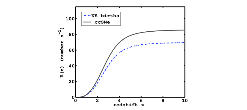
Figure 1: The total number of core collapse supernovae (ccSNe) events and neutron star (NS) births occurring per unit time within the comoving volume out to redshift z.

We assume that each ccSN results in either a NS or a BH, and integrate Eq. (1) over a NS (ccSNe) progenitor mass range of $8M_{\odot}-25\hskip 2.84526pt(100)M_{\odot}$ (Smartt, 2009). Fig. 1 shows the evolving ccSNe event rate as well as the NS formation rate. For the total rate of ccSNe and NS formation out to $z=10$ a maximum value is obtained as 85 $\rm{s}^{-1}$ and 69 $\rm{s}^{-1}$ respectively, with negligible contribution for $z>6$.

3 Stochastic gravitational wave background

To obtain the stochastic background, besides knowing the GW event rate we still need the average source spectrum. The energy flux per unit frequency emitted by a source at luminosity distance $d_{L}(z)$ is:

$$f(\nu_{\rm{obs}},z)=\frac{1}{4\pi d_{L}(z)^{2}}\frac{dE_{\rm{GW}}}{d\nu}(1+z),$$ (2)

where $dE_{\rm{GW}}/{d\nu}$ is the spectral energy density and $\nu$ is the frequency in the source frame which is related to the observed frequency by $\nu=\nu_{\rm{obs}}(1+z)$.

Combining Eq. (1) and Eq. (2) we can obtain the closure energy density $\Omega_{\rm{GW}}$ of the SGWB:

$$\Omega_{\rm{GW}}(\nu_{\rm{obs}})=\frac{\nu_{\rm{obs}}}{c^{3}\rho_{c}}\int_{0}^{10}[f(\nu_{\rm{obs}},z)(dR/dz)]dz,$$ (3)

where $\rho_{c}$ is the cosmological critical energy density.

One particular obstacle in estimating the SGWB comes from uncertainties in the source spectra. Fortunately, for a stochastic background detailed structures of source spectra are not important due to the following two facts.

Firstly the smearing of the spectrum by redshift means that a SGWB cannot be sharply peaked. Any narrow spectral details are greatly broadened. For example, if all sources emitted a narrow spectrum at 1 kHz, the resulting stochastic background is broadly peaked at 600 Hz with half-width $\sim 600$ Hz assuming our source rate evolution model. When individual sources create a stochastic background, redshift washes out most of the detailed structure.

Secondly a stochastic background consists of an average over a very large number of sources. For example, the frequency spectrum of a SGWB obtained from one-year cross correlation would be produced by the superposition of more than $10^{9}$ individual events. Given that source spectra are likely to vary with progenitor masses and angular momentum, any fine spectral detail will be averaged. In addition the BH formation spectrum scales inversely with BH mass, so again the average source will be smoothed and broadened assuming a continuous distribution of BH masses.

For the above two reasons a much simpler generic spectrum can be adopted for an average source. We go on to show that a Gaussian spectrum is a suitable approximation where $dE_{\rm{GW}}/{d\nu}$ is given by:

$${dE_{\rm{GW}}\over{d\nu}}=A\exp\bigg{[}-\frac{(\nu-\nu_{0})^{2}}{2{\Delta}^{2}}\bigg{]},$$ (4)

with amplitude $A$, peak frequency $\nu_{0}$, half-width $\Delta$.

Many of the modelling predictions show a range of spectral density varying over many orders of magnitude. However only the largest peaks in the source spectra contribute significantly to the stochastic background. For most predicted source waveforms one can obtain a very similar stochastic background from a Gaussian source spectrum. We have compared the resultant SGWB from 72 source models of Ott et al. (2004) with the signals obtained using a Gaussian approximation. We find, through comparison of the frequency integrated energy in the peak decade, that $87\%$ of our models are consistent to within $10\%$.

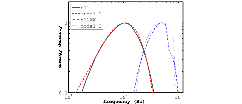
Figure 2: The relative spectral distribution of the SGWB from NS core collapse assuming two Gaussian source spectra (model 1 and model 2 ) and two simulated waveforms: s11A500B0.5 (denoted as s11) from Ott et al. (2004) and s11WW from Ott et al. (2006). Here s11 indicates a $11M_{\odot}$ presupernova model and we refer readers to the original papers for details of the simulations. We adopt the NS formation rate in Fig. 1 and scale the energy density of the SGWB to an arbitrary logarithmic scale. As only the strongest part of the background is essential to estimate an upper limit, we show only the highest decade of the relative stochastic background.

For illustration, in Fig. 2. we determine the SGWB based on two different GW emission mechanisms: firstly rotating core-collapse and bounce based in model s11 of Ott et al. (2004); secondly post collapse emission from accretion and turbulence driven proto-NS oscillations (acoustic mechanism) using model s11WW of Ott et al. (2006). The plot shows that for the highest decade, a Gaussian source spectrum given by Eq. (4) with $\nu_{0}=175$ Hz, $\Delta=120$ Hz (model 1) can produce a GW background with a spectral distribution comparable to that obtained using s11 (with a relative error $1.9\%$). Similarly, the SGWB determined using s11WW can also be well estimated (within $16.1\%$) by using a source model 2, with $\nu_{0}=860\hskip 2.84526pt\rm{Hz},\Delta=130\hskip 2.84526pt\rm{Hz}$. Although the exact spectral shape is not reproduced for model 2, we argue that the precise shape of the SGWB is not essential to obtain upper limits.

For above reasons in this paper, rather than adopt predicted spectra and determine the GW background, we have chosen to adopt a generic spectrum which takes into account the range of spectral predictions and use this to obtain an observational upper limit on the average GW production of ccSNe. Taking into account the range of progenitor masses and angular momentum, we would expect that the average source spectrum should be wider than those corresponding to particular simulations.

Based on the simulated ccSNe spectra of Dimmelmeier et al. (2008) (see Table 1 of Ott (2009)); and on spectra resulting from BH births from Sekiguchi & Shibata (2005), for which typical peak frequencies occur at around 1 kHz; we consider three Gaussian source spectra with the following parameters: a) $\nu_{0}=200\hskip 2.84526pt\rm{Hz},\Delta=200\hskip 2.84526pt\rm{Hz}$; b) $\nu_{0}=500\hskip 2.84526pt\rm{Hz},\Delta=400\hskip 2.84526pt\rm{Hz}$ and c) $\nu_{0}=800\hskip 2.84526pt\rm{Hz},\Delta=500\hskip 2.84526pt\rm{Hz}$ (denoted as model a, b and c respectively). In the next section we will use the above three generic source models to compare the SGWB from cosmological ccSNe with the LV limit.

4 Upper limits on the gravitational wave production of core collapse supernovae

We define the average GW production of ccSNe as: $E_{\rm{GW}}=\epsilon\cdot M_{\odot}c^{2}$ where $\epsilon$ is the average energy production in solar rest mass units and the total energy $E_{\rm{GW}}$ is distributed as Eq. (4). We obtain an upper limit on $\epsilon$ by scaling the SGWB calculated from a Gaussian average source model to produce a comparable signal-to-noise ratio (SNR) to that of a frequency-independent flat GW background. Assuming Gaussian noise in each of two cross-correlated detectors separated by less than one reduced wavelength, the optimal SNR after correlating outputs of two detectors during an integration time T is given by an integral over frequency $f$ (Allen & Romano, 1999, Eq. 3.75):

$$\left({S\over N}\right)^{2}={9H_{0}^{4}\over 50\pi^{4}}T\int_{0}^{\infty}df\>{\gamma^{2}(f)\Omega_{\rm{GW}}^{2}(f)\over f^{6}P_{1}(f)P_{2}(f)}\ ,$$ (5)

with $P_{1}(f)$ and $P_{2}(f)$ the power spectral noise densities of the two detectors and $\gamma(f)$ the overlap reduction function determined by the relative locations and orientations of two detectors (Flanagan, 1993). Here we adopt an integration time of 292 days and $\gamma(f)$ for LIGO H1-L1 calculated using Eq. (3.26) of Allen et al. (2002). We calculate Eq. (5) in the frequency band $(41.5-169.25)\hskip 2.84526pt\rm{Hz}$ using representative noise spectra. We find that the SNR given by Eq. (5) is 2.58 for a flat stochastic background $\Omega_{\rm{GW}}=6.9\times 10^{-6}$. In order to achieve the same SNR the average GW production $\epsilon$ is required to be $0.49$, $1.08$ and $1.98$ assuming source model a, b and c respectively.

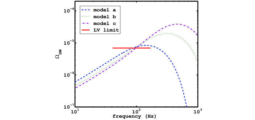
Figure 3: The upper limit on SGWB and GW background from cosmological ccSNe assuming three different Gaussian source models (see text). The models have been scaled to produce the same SNR within (41–169) Hz as that of a flat frequency-independent background (LV limit).

Fig. 3 shows the LV limit along with the predicted stochastic backgrounds from ccSNe for the three average source models. The strongest constraint is obtained when individual sources emits gravitational radiation at a peak frequency near LIGO’s most sensitive frequency band. This corresponds to $\epsilon\leq 0.49$ ($E_{\rm{GW}}=8.8\times 10^{53}\hskip 2.84526pt\rm{ergs}$) assuming an average source spectrum given by model a. Note that this limit is higher than the available energy ($\sim 3.0\times 10^{53}\hskip 2.84526pt\rm{ergs}$) for any kind of emission in a ccSNe event which is set by the binding energy of the final NS. If the source peak frequency increases, as in models b and c we obtain somewhat higher limits (1.08 and 1.98 respectively) for $\epsilon$. Fig. 3 also illustrates that stronger constraints can be obtained if stochastic background limits at higher frequencies are available.

It is important to consider the effect of other stochastic background sources. We can be reasonably certain that the true stochastic background contains contributions from compact binary coalescences and individual spinning NSs. All these sources contribute GW energy in the relevant frequency band. Of these, the coalescing compact binaries are worth considering because significant fraction of system binding energy is expected to be converted to GWs. However, their event rate is much lower, about $10^{-3}$ of ccSNe rate (Sadowski et al., 2008; Abadie et al., 2010b; Belczynski et al., 2010). Thus applying similar methods to such systems will yield $10^{3}$ higher upper limit on the average GW production. We therefore only consider ccSNe in this study.

It is interesting to note that the LV limit is comparable to the minimum detectable GW energy density with two initial LIGO detectors predicted some years ago - $\Omega_{\rm{GW}}\sim 5\times 10^{-6}$ (see, e.g., Allen, 1996; Maggiore, 2000). A world-wide network of advanced detectors have been planned or proposed, including Advanced LIGO (Harry et al., 2010), Advanced Virgo (Acernese et al., 2009), LCGT (Kuroda et al., 2010) and AIGO (Barriga et al., 2010). Additionally design studies for a third-generation GW observatory, Einstein Telescope (ET; Punturo et al., 2010), are well underway with a target sensitivity 100 times better than current instruments. While limits obtained here are far away from being able to test GW emission mechanisms of ccSNe, future measurements will lead to great improvements in this regard. For instance, Advanced LIGO will be able to detect or to set a much stronger limit on the stochastic background at the level of $\Omega_{\rm{GW}}\geq 9\times 10^{-10}$ (Advanced LIGO Team, 2007). This will imply an upper limit on the GW production of ccSNe as low as $\sim 10^{-5}\hskip 2.84526ptM_{\odot}c^{2}$. For ET, the minimum detectable value $\Omega_{\rm{GW}}\sim 5\times 10^{-12}$ (Sathyaprakash & Schutz, 2009) corresponds to a limit $\sim 10^{-7}\hskip 2.84526ptM_{\odot}c^{2}$, which is in the range of predictions from various ccSNe simulations.

5 Conclusions

We have shown that upper limits on the stochastic background of GWs can be used to set limits on the GW energy production in ccSNe. This result is the first upper limit for GW production averaged over all core collapse events out to z $\sim 10$. The upper limit is in the range $(0.49-1.98)\hskip 2.84526ptM_{\odot}c^{2}$ depending on the average source spectrum. Our result represents an average over both space and cosmic time, thereby including an average over possible evolutionary effects in GW production. It is higher than the upper limit on the available energy for explosion in a core collapse event. However second and third generation GW detectors will enable tighter constraints to be set on the GW emission from such systems. Using our methods the predicted upper limits on the average GW production from ccSNe will be $10^{-5}\hskip 2.84526ptM_{\odot}c^{2}$ and $10^{-7}\hskip 2.84526ptM_{\odot}c^{2}$ for Advanced LIGO and ET respectively.

Compact binary coalescence events are not considered in the above limit because their event rate is very low in comparison with ccSNe. However, at the expected improved limits from Advanced LIGO and ET, it will be possible to consider GW backgrounds from other sources like compact binary coalescences.

It would be interesting to compare our upper limits with those on the fraction of stellar core rest mass converted to GWs obtained by averaging GW detector outputs over time periods associated with nearby ccSNe (Finn, 2001). Such methods have already been used to set upper limits on the total energy emitted in GWs for one particular astrophysical event during searches for GW bursts. For example, Abbott et al. (2008b) placed an upper limit of $1.6\times 10^{4}\hskip 2.84526ptM_{\odot}c^{2}$ on the total GW energy for GRB 050223 (D $\approx 3.5\hskip 2.84526pt\rm{Gpc}$) which was considered to be associated with a core collapse. In Abbott et al. (2010b), a GW energy limit for GRB 070201 was given as $1.15\times 10^{-4}\hskip 2.84526ptM_{\odot}$ at 150 Hz assuming a position of M31 (770 kpc). As we can see such limits depend strongly on the knowledge of source distance. Abadie et al. (2010a) set a limit on the total energy of one GW burst event (assuming a sine-Gaussian signal) that would be detectable with the current LIGO-Virgo detectors as $1.8\times 10^{-8}\hskip 2.84526ptM_{\odot}c^{2}$ and $4.6\times 10^{-3}\hskip 2.84526ptM_{\odot}c^{2}$ for a typical Galactic distance (10 kpc) and the Virgo cluster (16 Mpc) respectively.

This method suffers from the poor time resolution for the collapse event (unless timed by detected neutrinos) and a small sample of events during the period that GW data are available. However with the improvements of detector sensitivities, stronger upper limits or even positive detection of GWs from ccSNe will be possible based on single or small numbers of events in the future.

References

- Abadie et al. (2010a) Abadie J. et al., 2010a, Phys. Rev. D, 81, 102001
- Abadie et al. (2010b) Abadie J. et al., 2010b, CQG, 27, 173001
- Abadie et al. (2010c) Abadie J. et al., 2010c, preprint (arXiv:1006.2535)
- Abadie et al. (2010d) Abadie J. et al., 2010d, preprint (arXiv:1007.3973); http://www.ligo.caltech.edu/
- Abbott et al. (2008a) Abbott B. et al., 2008a, ApJ, 683, L45
- Abbott et al. (2008b) Abbott B. et al., 2008b, Phys. Rev. D, 77, 062004
- Abbott et al. (2008c) Abbott B. et al., 2008c, Phys. Rev. Lett., 101, 211102
- Abbott et al. (2009a) Abbott B. P. et al., 2009a, Phys. Rev. D, 80, 047101
- Abbott et al. (2009b) Abbott B. P. et al., 2009b, Nature, 460, 990
- Abbott et al. (2010a) Abbott B. P. et al., 2010a, ApJ, 713, 671
- Abbott et al. (2010b) Abbott B. P. et al., 2010b, ApJ, 715, 1438
- Accadia et al. (2010) Accadia T. et al., 2010, CQG, submitted (arXiv:1009.5190); http://www.virgo.infn.it/
- Acernese et al. (2009) Acernese F. et al., 2009, Advanced Virgo baseline design, Virgo Internal Note VIR-0027A-09; http://wwwcascina.virgo.infn.it/advirgo/
- Advanced LIGO Team (2007) Advanced LIGO Team, 2007, Advanced LIGO reference design; http://www.ligo.caltech.edu/docs/M/M060056-10.pdf
- Allen (1996) Allen B., 1996, Lectures at Les Houches School, arXiv:gr-qc/9604033
- Allen et al. (2002) Allen B., Creighton J. D., Flanagan É. É., Romano J. D., 2002, Phys. Rev. D, 65, 122002
- Allen & Romano (1999) Allen B., Romano J. D., 1999, Phys. Rev. D, 59, 102001
- Arai et al. (2008) Arai K. et al., 2008, Journal of Physics Conference Series, 120, 032010; http://tamago.mtk.nao.ac.jp/
- Baldry & Glazebrook (2003) Baldry I. K., Glazebrook K., 2003, ApJ, 593, 258
- Barriga et al. (2010) Barriga P. et al., 2010, CQG, 27, 084005; http://www.aigo.org.au/
- Bastian et al. (2010) Bastian N., Covey K. R., Meyer M. R., 2010, ARA&A, 48, 339
- Belczynski et al. (2010) Belczynski K. et al., 2010, ApJ, 715, L138
- Baiotti et al. (2007) Baiotti L., Hawke I., Rezzolla L., 2007, CQG, 24, 187
- Baiotti & Rezzolla (2006) Baiotti L., Rezzolla L., 2006, Phys. Rev. Lett., 97, 141101
- Blair & Ju (1996) Blair D., Ju L., 1996, MNRAS, 283, 648
- Coward et al. (2001) Coward D. M., Burman R. R., Blair D. G., 2001, MNRAS, 324, 1015
- Dimmelmeier et al. (2002) Dimmelmeier H., Font J. A., Müller E., 2002, A&A, 393, 523
- Dimmelmeier et al. (2008) Dimmelmeier H., Ott C. D., Marek A., Janka H.-T., 2008, Phys. Rev. D, 78, 064056
- Ferrari et al. (1999) Ferrari V., Matarrese S., Schneider R., 1999, MNRAS, 303, 247
- Finn (2001) Finn L. S., 2001, arXiv:gr-qc/0104042
- Flanagan (1993) Flanagan E., 1993, Phys. Rev. D, 48, 2389
- Fryer et al. (2001) Fryer C. L., Woosley S. E., Heger A., 2001, ApJ, 550, 372
- Grote et al. (2010) Grote H. et al, 2010, CQG, 27, 084003; http://www.geo600.uni-hannover.de
- Harry et al. (2010) Harry G. M. et al., 2010, CQG, 27, 084006
- Hopkins & Beacom (2006) Hopkins A. M., Beacom J. F., 2006, ApJ, 651, 142
- Houser et al. (1994) Houser J. L., Centrella J. M., Smith S. C., 1994, Phys. Rev. Lett., 72, 1314
- Howell et al. (2004) Howell E., Coward D., Burman R., Blair D., Gilmore J., 2004, MNRAS, 351, 1237
- Kawamura (2010) Kawamura S., 2010, CQG, 27, 084001
- Kuroda et al. (2010) Kuroda K. et al., 2010, CQG, 27, 084004; http://gw.icrr.u-tokyo.ac.jp/lcgt/
- Leonor et al. (2010) Leonor I. et al., 2010, CQG, 27, 084019
- Maggiore (2000) Maggiore M., 2000, Phys. Rep., 331, 283
- Müller (1997) Müller E., 1997, CQG, 14, 1455
- Ott (2009) Ott C. D., 2009, CQG, 26, 063001
- Ott et al. (2006) Ott C. D., Burrows A., Dessart L., Livne E., 2006, Phys. Rev. Lett., 96, 201102
- Ott et al. (2004) Ott C. D., Burrows A., Livne E., Walder R., 2004, ApJ, 600, 834
- Punturo et al. (2010) Punturo M. et al., 2010, CQG, 27, 194002; http://www.et-gw.eu/
- Regimbau & Mandic (2008) Regimbau T., Mandic V.,2008, CQG, 25, 184018
- Sadowski et al. (2008) Sadowski A. et al., 2008, ApJ, 676, 1162
- Sathyaprakash & Schutz (2009) Sathyaprakash B., Schutz B. F., 2009, Living Rev. Relativity, 12, 2
- Sekiguchi & Shibata (2005) Sekiguchi Y., Shibata M., 2005, Phys. Rev. D, 71, 084013
- Smartt (2009) Smartt S. J., 2009, ARA&A, 47, 63
- Thorne (1987) Thorne K. S., 1987, Gravitational Radiation, in 300 years of Gravitation, edited by S. Hawking and W. Israel, pages 330-458. Cambridge University Press, Cambridge, UK
- van Elewyck et al. (2009) van Elewyck V. et al., 2009, International Journal of Modern Physics D, 18, 1655