Stress Orientation Confidence Intervals from Focal Mechanism Inversion

Abstract.

The determination of confidence intervals of stress orientation is a crucial element in the discussion of homogeneity or heterogeneity of the stress field under study. The error estimates provided by the grid search method Focal Mechanism Stress Inversion of Gephart and Forsyth (1984) have been shown to be too wide but the reasons for this failure have escaped elucidation.

Through the use of directional statistics and synthetic focal mechanisms, I show that the grid search methodology does yield appropriate uncertainty estimates. The direct perturbation of the synthetic focal mechanisms introduces bias which leads to confidence intervals which become increasingly too wide as the amount of perturbation increases. The synthetic data also show at what point the method fails to overcome this bias and when confidence intervals will be too wide. The indirect perturbation of the focal mechanisms by perturbing the generating deviatoric stress tensor generates synthetic data devoid of bias. Inversion of these data sets yields correct confidence intervals.

The Focal Mechanism Stress Inversion method is vindicated as a highly effective method, and with the use of appropriate directional statistics, its results can be assessed and homogeneity or heterogeneity of the stress field can be discussed with confidence.

1. Introduction

Gephart and Forsyth (1984) proposed a grid search method of inverting focal mechanisms to obtain the stress tensor (focal mechanisms stress inversion, henceforward FMSI), in which stress field parameters are tried systematically against the focal mechanism orientations and the misfit calculated. They defined the misfit as the sum of the minimum angle needed to bring the slip direction of each focal mechanism into line with the resolved shear stress on the fault plane. Both planes of each focal mechanism are tried and the smallest misfit serves to differentiate fault plane from auxiliary plane. They incorporated the one-norm measure as misfit criterion, adopting the methodology proposed by Parker and McNutt (1980). Different techniques for such inversions had been proposed already, and Gephart (1990b) discussed their relative merits, particularly in the context of focal mechanisms and the problems associated with the presence of two nodal planes.

Michael (1987) proposed a different method, relying on a linearisation and bootstrapping to invert focal mechanisms for stress tensor calculation. He drew attention to some differences in the size of the confidence intervals obtained by these two different methods.

It became quickly apparent that the discrepancies in confidence intervals had major repercussions on the study of actual stress fields. Different methods led different groups of researchers to different conclusions regarding the spatial and temporal variation in the stress regime in Southern California. This unsatisfactory state of affairs led Hardebeck and Hauksson (2001) to test thoroughly the different methodologies using synthetic data. They showed that the confidence intervals estimated by FMSI were much too large, but they did not succeed in determining the reasons for such overestimates.

Here, I attempt to uncover the nature of the confidence intervals estimated by FMSI by investigating the Hardebeck and Hauksson (2001) analysis. Initial attempts to resolve the problem of these too wide confidence intervals brought to light some inaccuracies in the derivation and application of the one-norm measure as proposed by Parker and McNutt (1980) and applied by Gephart and Forsyth (1984) and Hardebeck and Hauksson (2001) (Revets, 2009). These corrections proved insufficient to lessen significantly the width of the confidence intervals (Hardebeck, pers. comm.).

This left two avenues of investigation: the nature of the statistics used to calculate the confidence intervals, and the methodology of calculating the synthetic data used to test the method.

2. Directional statistics

Fisher (1953) pointed out that the initial development of the theory of errors by Gauss aimed to help astronomers and surveyors with their accurate angular measurements. Because of the accuracy of their measurements, the linear approximation to which Gauss resorted was both appropriate and effective. However, when the errors become substantial, the linear approximation is no longer valid and the topological framework has to be taken into account.

The spherical mean direction $R$ and variance $S$ are defined as

(1) $$R^{2}=\big{(}\sum_{i=1}^{N}l_{i}\big{)}^{2}+\big{(}\sum_{i=1}^{N}m_{i}\big{)}^{2}+\big{(}\sum_{i=1}^{N}n_{i}\big{)}^{2}$$

and

(2) $$S=(N-R)/N$$

where $l_{i}$, $m_{i}$, $n_{i}$ are the direction cosines of the angular measurements (Mardia, 1972).

The spherical equivalent of the normal distribution is the Fisher distribution (Fisher, 1953), defined by

(3) $$df=\frac{\kappa}{2\sinh\kappa}e^{\kappa\cos\theta}\sin\theta d\theta$$

in which $\kappa$ is a measure of concentration. When $\kappa$ approaches zero, the distribution becomes uniform over the entire sphere whereas for $\kappa$ large, the distribution is confined to a small region of the sphere around the maximum. In the latter case, the distribution comes close to a two-dimensional (isotropic) normal distribution where $\kappa$ plays the role of the inverse of the variance.

The maximum likelihood estimate of $\kappa$ for the distribution on a sphere is for larger values of $\kappa$

(4) $$\mathrm{bar}{R}=\frac{I_{1.5}(\kappa)}{I_{0.5}(\kappa)}$$

where $I_{n}$ is the modified Bessel function of the first kind and the n-th order (Watson, 1944) and $\mathrm{bar}{R}$ the mean of $R$ (Watson and Williams, 1956; Mardia, 1972). For large values of $\kappa$, the most likely value is given by

(5) $$\kappa=\frac{N-1}{N-R}$$

(Fisher, 1953; Watson, 1960).

Confidence intervals for $\kappa$ can be determined from the relation

(6) $$2\kappa(N-R)=\chi^{2}_{2N-2}$$

(Watson and Williams, 1956; Mardia, 1972).

3. Application to stress tensor inversion

To calculate and test the confidence intervals of stress tensors inverted from focal mechanisms, I adapted and modified the method used by Hardebeck and Hauksson (2001), taking particular care to adhere to the strictures and requirements of directional statistics.

3.1. Generating synthetic focal mechanisms

Sets of focal mechanisms are made up from spherically randomly oriented fault planes with slip directions determined by a chosen stress tensor. The azimuth of the fault planes is chosen from uniformly distributed random numbers in the $[0,2\pi]$ interval, while the dip is randomly taken out of the $[0,1]$ interval through

(7) $$d_{i}\in\arccos[0,1]$$

to avoid the (spherical) bias that the direct selection from the $[0,\pi/2]$ interval would cause. Sets contain either 20, 50 or 100 fault planes.

The direction of slip on the fault plane given the stress tensor follows from the formalism of Ramsey and Lisle (1983)

(8) $$l(m^{2}\phi+n^{2}):m(n^{2}(1-\phi)-l^{2}\phi):-n(l^{2}+m^{2}(1-\phi))$$

where $l$, $m$, $n$, are the direction cosines of the fault plane in the stress tensor reference frame and $\phi$ is the stress shape ratio

(9) $$\phi=\frac{\sigma_{1}-\sigma_{2}}{\sigma_{1}-\sigma_{3}}$$

This direction of slip, as the normal to the auxiliary plane, completes the definition of the focal mechanism.

3.2. Generating error

I used a Fisher distribution to generate random directions and angles to perturb orientations (Mardia, 1972, p. 231), and used quaternions to carry out the required rotations. Figure 1 shows an example of such Fisher distributed error angles and orientations plotted on a polar Schmidt net. Values of $\kappa$ for the Fisher distribution which correspond to perturbations of 1 °, 5 °, 10 °, 15 ° and 20 ° can be obtained through interpolation from equation 4.

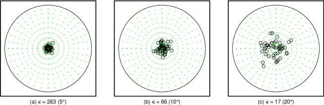
Figure 1. Polar Schmidt plots of examples of Fisher distributed errors, as used to perturb the generating stress tensor. The crosses are 10 ° apart

There are two ways in which to incorporate errors in the synthetic data set. There is the natural way of perturbing each focal mechanism directly. It is also possible to perturb the generating stress tensor before calculating the slip direction on each fault plane in the data set. The assumptions behind these two ways are very different, and I discuss their implications, statistical as well as physical, following the simulation results.

3.3. Data inversion and statistics

Each synthetic data set is then processed by FMSI, which inverts the focal mechanisms to obtain the stress tensor. Thanks to FMSIETAB, part of the FMSI suite of programs, it is possible to generate a list of angular deviation between each fault plane and any given stress tensor. Such lists, comparing the deviations between focal mechanisms with the generating stress tensor as well as with the inverted stress tensor allow the calculation of the respective spherical mean $R$ and the concentration parameter $\kappa$, using equations 1 and 5. Each combination of $N$ fault planes with the different amounts of perturbation is replicated 50 times.

Hardebeck and Hauksson (2001) proposed that for appropriate confidence intervals the correct stress tensor should fall within the P confidence region for an approximate proportion P of all the data sets. A plot of (sorted) probabilities versus proportion should be a diagonal. If the confidence intervals are too wide, the plot will show a curve above the diagonal and too narrow confidence intervals will result in a curve below the diagonal. These graphs are an equivalent of P-P plots (Wilk and Gnanadesikan, 1968; Holmgren, 1995). P-P plots are scatter plots of $F_{1}(q_{i}),F_{2}(q_{i})$, where $F_{1}(q_{i})$ is obtained by applying

(10) $$F_{1}(F_{2}^{-1}(p_{i}))$$

to the two empirical cumulative density functions ($F$) of the two data sets being compared. Here, I show P-P plots which compare the cumulative density function of the misfit against the inverted stress tensor with the cumulative density function of the misfit against the generating stress tensor.

Gephart (1990b) proposed a modification of the method proposed by Zizicas (1955) to represent the orientation of a fault plane with respect to the principal stress directions. Gephart’s unscaled Mohr Sphere uses the stress components $\sigma$, $\tau_{S}$ and $\tau_{b}$ as axes.

The maximum shear stress and mean normal stress are respectively

(11) $$\tau_{m}=\frac{\sigma_{1}-\sigma_{3}}{2},\quad\sigma_{m}=\frac{\sigma_{1}+\sigma_{3}}{2}$$

The absolute values of the stress tensor are inaccessible, but the relative magnitudes of the principal stress components can be calculated. Their relation is given by

(12) $$\phi=\frac{\sigma_{2}-\sigma_{1}}{\sigma_{3}-\sigma_{1}}$$

The three normalized stress components acting on a fault plane can be described as

(13) $$\sigma=\frac{\sigma^{\prime}_{11}-\sigma_{m}}{\tau_{m}},\quad\tau_{b}=\frac{\sigma^{\prime}_{12}}{\tau_{m}},\quad\tau_{s}=\frac{\sigma^{\prime}_{13}}{\tau_{m}}$$

and are completely determined by the dimensionless quantities $\phi$ and $\beta_{ij}$, where $\beta_{ij}$ is determined from

(14) $$\sigma^{\prime}_{ij}=\sigma_{kl}\beta_{ik}\beta{jl}$$

which relates the stress tensor components between the coordinate systems of the fault plane and of the regional stress tensor. The shear stress will match the slip direction on a plane when $\sigma^{\prime}_{12}$ is zero (Gephart, 1990b).

Mohr Sphere plots of fault planes are often illuminating and are of great assistance with the interpretation of the inversions. This is also the case with the differently treated synthetic data sets, and I include a number of such Mohr Sphere plots for some of the data used.

4. Results

4.1. P-P Plots

The P-P plots obtained from the new analyses presented here (Figure 2–4) show a considerable improvement for the method compared to the results obtained by Hardebeck and Hauksson (2001). It appears that the change from linear statistics to directional statistics improves the appropriateness of the confidence interval estimation significantly. The graphs show a number of trends, including some unexpected ones.

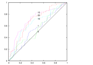
(a) Focal mechanism perturbation

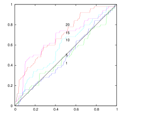
(b) Stress tensor perturbation

Figure 2. P–P plot of $\kappa$ for $N$=20, with the generating tensor values along the x-axis and the inverted tensor values along the y-axis. The amount of perturbation in degrees is shown on each individual curve.

The most obvious, and expected, trend is a decrease in precision of the confidence interval estimates as the amount of error increases. This trend is present in each individual graph (Figures 2–4).

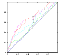
(a) Focal mechanism perturbation

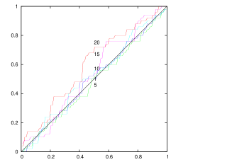
(b) Stress tensor perturbation

Figure 3. P–P plot of $\kappa$ for $N$=50, with the generating tensor values along the x-axis and the inverted tensor values along the y-axis. The amount of perturbation in degrees is shown on each individual curve.

What is unexpected is that if the estimate of the confidence intervals is imprecise, it is systematically too large. In the face of error, the method performs better than one would expect, something that was very pronounced in the study by Hardebeck and Hauksson (2001).

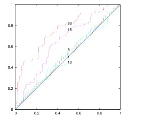
(a) Focal mechanism perturbation

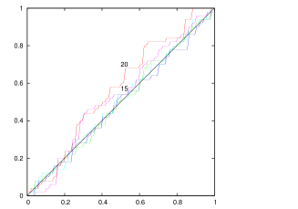
(b) Stress tensor perturbation

Figure 4. P–P plot of $\kappa$ for $N$=100, with the generating tensor values along the x-axis and the inverted tensor values along the y-axis. The amount of perturbation in degrees is shown on each individual curve.

The other noticeable and expected trend is an increase in precision of the confidence interval estimates as the number of focal mechanisms increases. This trend is very pronounced in graphs of the stress tensor perturbation set (Figures 2b, 3b and 4b). The graphs of the focal mechanism perturbation set (Figures 2a, 3a and 4a) show an increase in precision for the smaller amounts of error, but an unexpected decrease for the larger amounts of error.

There is also a clear tendency for an increased precision for the stress tensor perturbation sets against their focal mechanism perturbation equivalents (the (b) subfigure against the (a) subfigure for each of Figures 2, 3 and 4).

4.2. Mohr Sphere Projections

(a) Generating Stress Tensor

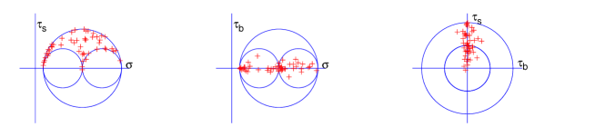
(b) Inverted Stress Tensor

Figure 5. Mohr Sphere projections of the poles of the fault planes relative to the stress components defined by the respective stress tensor. The fault planes have been subjected to a 1 ° Fisher distributed perturbation.

(a) Generating Stress Tensor

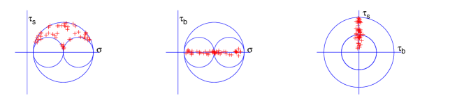
(b) Inverted Stress Tensor

Figure 6. Mohr Sphere projections of the poles of the fault planes relative to the stress components defined by the respective stress tensor. The stress tensor has been subjected to a 1 ° Fisher distributed perturbation.

The Mohr Sphere projections (Figures 5–8) are examples of 4 data set of 50 focal mechanisms which have undergone either a 1 ° (Figures 5 and 6) or a 15 ° (Figures 7 and 8) Fisher distributed amount of error. Each figure shows two sets of Mohr Sphere plots: one illustrating the fault planes against the generating stress tensor (or its spherical average when it was the generating stress tensor that underwent perturbation), and one showing the same set of fault planes against the inverted stress tensor calculated by FMSI.

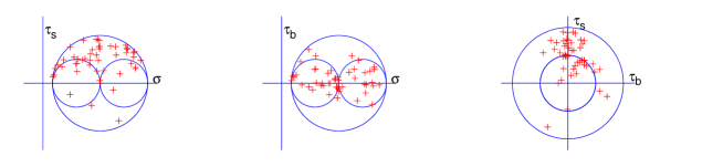
(a) Generating Stress Tensor

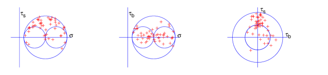
(b) Inverted Stress Tensor

Figure 7. Mohr Sphere projections of the poles of the fault planes relative to the stress components defined by the respective stress tensor. The fault planes have been subjected to a 15 ° Fisher distributed perturbation.

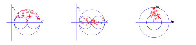
(a) Generating Stress Tensor

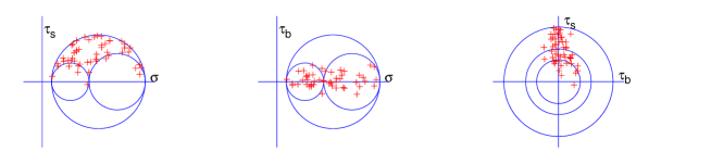
(b) Inverted Stress Tensor

Figure 8. Mohr Sphere projections of the poles of the fault planes relative to the stress components defined by the respective stress tensor. The stress tensor has been subjected to a 15 ° Fisher distributed perturbation.

The first trend which stands out is the larger amount of scatter on the Mohr Sphere projections for the fault plane perturbed data sets (Figures 5 and 7) compared to the projections for the stress tensor perturbed data sets (Figures 6 and 8) which is particularly noticeable on the $\sigma-\tau_{b}$ graphs. This increase in scatter includes the presence of fault planes with the wrong direction of slip ($\tau_{S}<0$, seen as crosses which plot below the X-axis in the $\sigma-\tau_{S}$ and $\tau_{b}-\tau_{S}$ graphs).

A second trend is the larger amount of change between the Mohr Sphere plots (going from the plot of the fault planes in the generating stress tensor Mohr Sphere to the Inverted tensor Mohr Sphere) for the data sets that have undergone fault plane perturbations compared to the data sets that have undergone stress tensor perturbation. There is more change visible going from the (a) subfigures to the (b) subfigures in Figures 5 and 7 than in Figures 6 and 8.

5. Discussion

Theoretical and statistical reasoning requires us to use directional statistics instead of linear statistics when we deal with focal mechanisms and deviatoric stress tensor inversion. The Fisher distribution and its properties are well established and its use in the present, theoretical study has been effective. The question does arise if this distribution is a good representation of actual seismological data.

Discussions of the distribution of data misfit to stress tensors in the literature (Gephart and Forsyth, 1984; Hardebeck and Hauksson, 2001; Wyss et al., 1992) consistently mention the non-normality of the data and refer qualitatively to exponential or Poisson distributions. Turning to spherical statistics resolves this issue immediately. The Fisher distribution, as given in equation 3, shows directly its exponential nature. The method adopted by Hardebeck and Hauksson (2001) for their simulations, in which they combine exponentially distributed dip angles with uniformly distributed azimuth angles, generates in effect a set of Fisher distributed orientations.

Since we are trying to assess the confidence intervals of the stress tensor inversion through simulations, we have to ensure that we use appropriate models and calculations to compare the perturbation distributions. It is highly instructive to compare the effects of injecting uncertainty into the simulations at two different points. It is for this reason that I opted to inject uncertainty or error in the focal mechanisms to test the inversion process by perturbing the orientation of the generating stress tensor, as well as the more intuitive approach of perturbing the orientation of the individual focal mechanisms directly.

The fault planes are chosen from uniform spherical random orientations (equation 7) and the direction of slip is calculated from the stress tensor according to equation 8. It is clear that the relation between orientation of any of the focal mechanisms and the stress tensor is highly non-linear. That non-linearity necessarily also applies to any perturbation and in particular to the way in which it propagates in any calculation or inversion. It is incorrect to assume that a perturbation distribution applied to a set of focal mechanisms would translate to the same perturbation distribution of the inverted stress tensor. This effect can be clarly seen in the Mohr Sphere plots where the scatter is much larger in the plots of the data sets subjected to fault plane perturbation (Figures 5 and 7) than those subjected to tensor perturbation (Figures 6 and 8).

Comparing the dispersions of the data misfit to the inverted stress tensor with the dispersion of the perturbations in this case will be misleading. The dispersion of the stress tensor orientations (consistent with the perturbed focal mechanisms) is necessarily larger than the dispersion used perturb the focal mechanisms. It is therefore not surprising that the inversion method will converge to the correct stress tensor more often than one would expect from the dispersion used. This problem can be avoided by letting the perturbation occur on the generating tensor, before generating the focal mechanisms. This effect is clearly shown by the contrast between the P-P plots of the data sets subjected to fault plane perturbation and the data sets subjected to stress tensor perturbation (respectively the (a) and (b) subplots in Figures 2–4).

Perturbing the fault planes directly in effect introduces bias into the data set because each of the perturbed fault planes appears to have been generated by a potentially very different stress tensor, including incompatibly oriented stress tensors. This bias contaminates the dispersion. Using this contaminated dispersion to measure the accuracy of the confidence intervals then leads to the erroneous conclusion that the inversion method overestimates the confidence intervals.

As far as simulations are concerned, the statistics can only legitimately be compared if they are commensurable. That is not the case when error is injected at the level of the individual fault plane. Unfortunately, this situation mirrors exactly what happens in the real world: the parameters describing a calculated focal mechanism are subject to error and uncertainty, not the generating stress tensor. Therefore, it may seem that the fact that FMSI yields correct confidence intervals only when the generating stress tensor is subjected to error, but fails to do so when focal mechanisms are error prone, is of no practical benefit.

The paradox can be resolved as follows. I have demonstrated that FMSI yields correct confidence intervals when the dispersions used to calculate the confidence intervals are commensurable. I have also shown that error in focal mechanisms introduces bias in the statistics of the population at hand. But thanks to the side-by-side simulations, it is possible to estimate to what extent this bias contaminates the calculations of FMSI. As one would expect from the law of large numbers (Révész, 1968), a statistic converges to its theoretical value as the population size increases. This can be seen very clearly in the P-P plots: the results of the simulations converge to the diagonal as the sample size increases. This is very obvious for the simulations in which the generating stress tensor was subjected to error (the (b) subplots in Figures 2–4). Closer scrutiny of the P-P plots of the simulations in which the focal mechanisms were subjected to perturbation shows a similar, albeit slower convergence (the (a) subplots in Figures 2–4). There is a trade-off between amount of error and population size: FMSI is capable of estimating confidence intervals correctly up to a certain amount of bias. Figure 2a shows that for populations of 20 focal mechanisms, FMSI is capable of dealing with an average of 5 ° of error on the focal mechanisms. This increases to 10 ° for 50 focal mechanisms (Figure 3a) and to 12–13 ° for 100 focal mechanisms (Figure 4a).

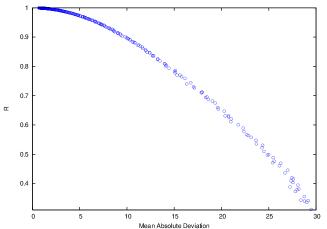
Figure 9. Empirical relation between the $\mathrm{bar}{R}$ values and mean absolute deviation ( °) for the Fisher Distribution

The calculations by FMSI do not use directional statistics and the questions arises if a simple conversion is possible from the dispersion measure given by FMSI to directional statistics and allow the application of the correct calculation of confidence intervals as shown here. The mean deviation calculated by FMSI is an average of angles while the circular mean is the average of the cosines of angles. There is no analytical formula to go from one to the other. Nevertheless, there is a clear relation between the mean absolute deviation and $\mathrm{bar}{R}$ for the Fisher Distribution (see Figure 9) and graphs of this nature could be used to estimate values which can then be used to determine the confidence intervals. The correct procedure, albeit more calculation intensive, is to use the list of individual focal mechanism misfits (which can be obtained through FMSIETAB) and to apply equation 6.

6. Conclusions

The processing and discussion of data from focal mechanisms and deviatoric stress tensors should use directional statistics.

The genesis of synthetic data in the context of stress tensor inversion requires very careful scrutiny of how perturbation is incorporated.

The inversion of deviatoric stress tensors from focal mechanisms using the grid search method of Gephart yields reliable confidence intervals if correct, directional statistics are used. When calculated misfits are small for moderate to large numbers of focal mechanisms, the method recovers the true stress tensor and confidence intervals become superfluous.

Gephart’s FMSI is a highly effective and reliable method for stress tensor inversion.

7. Data and Resources

The synthetic data, data inversion and additional calculations relied on a combination of Bash shell scripts and procedures written for the Octave program (Eaton, 2002). The FMSI suite of programs is in the public domain and made available by Gephart (1990a). The fortran source code is freely available from www.geo.cornell.edu/pub/FMSI.

References

- Eaton (2002) Eaton, J. W. (2002). GNU Octave Manual, Network Theory Limited.
- Fisher (1953) Fisher, R. A. (1953). Dispersion on a sphere, Proc. Roy. Soc. Lond., Ser. A 217, 295–305.
- Gephart (1990a) Gephart, J. W. (1990a). FMSI: a FORTRAN program for inverting fault/slickenslide and earthquake focal mechanism data to obtain the regional stress tensor, Comp. Geosci. 16, 953–989.
- Gephart (1990b) Gephart, J. W. (1990b). Stress and the direction of slip on fault planes, Tectonics 9, no. 4, 845–858.