Dependence of the spectrum of a quantum graph on vertex conditions and edge lengths

Abstract.

We study the dependence of the quantum graph Hamiltonian, its resolvent, and its spectrum on the vertex conditions and edge lengths. In particular, several results on the analyticity and interlacing of the spectra of graphs with different vertex conditions are obtained and their applications are discussed.

1. Introduction

Graph models have long been used as a simpler setting to study complicated phenomena. Quantum graphs in particular have recently gained popularity as models for thin wires, eigenvalue statistics of chaotic systems and properties of the nodal domains of eigenfunctions. We refer the interested reader to the recent reviews [17, 10, 19] and collections of papers [3, 7].

A quantum graph is a metric graph equipped with a self-adjoint differential “Hamiltonian” operator (usually of Schrödinger type) defined on the edges and matching conditions specified at the vertices. Every edge of the graph has a length assigned to it. In this manuscript we establish several results concerning the general properties of the spectrum of the Hamiltonian as a function of the parameters involved: the edge lengths and matching (vertex) conditions. In Section 2 we introduce the standard notions related to quantum graphs, vertex conditions, and quadratic forms of the corresponding Hamiltonians. The most widely used example of the vertex conditions, the $\delta$-type condition, is described in some detail. The results presented in Section 3 concern the analyticity of the spectrum as a function of the parameters involved: vertex conditions and edge lengths. Analytic dependence on the potential (as an infinite-dimensional parameter) can also be established by the methods used in the Section, but we omit this to keep the presentation simple. In Section 4 we compute the derivative of an eigenvalue with respect to a variation in the length of an edge; this is an analogue of a well-known Hadamard variational formula. Derivative with respect to a parameter of a $\delta$-type condition is also computed.

Section 5 again focuses on the $\delta$-type condition at a vertex. Varying such a condition at a specified vertex or changing connectivity of the vertex we obtain families of spectra and study their interlacing properties. Eigenvalue interlacing (or bracketing) is a powerful tool in spectral theory with such well-known applications as the derivation of the asymptotic Weyl law, see [5]. In the graph setting, it allows one to estimate eigenvalue of a given graph via the eigenvalues of its subgraphs, which may be easier to calculate. Interlacing results on graphs have already been used in several situations [26, 2, 21]. We significantly generalize these results and put them in the form particularly suited for the applications. We discuss several applications. In particular, we give a simple derivation of the number of nodal domains of the $n$-th eigenfunction on a quantum tree and study irreducibility of the spectrum of a family of graphs obtained by varying $\delta$-type condition at one of the vertices.

2. Quantum graph Hamiltonian

Let $\Gamma=(\mathcal{V},\mathcal{E})$ be a graph with finite sets of vertices $\mathcal{V}=\{v_{j}\}$ and edges $\mathcal{E}=\{e_{j}\}$. We will assume that $\Gamma$ is a metric graph, i.e. every edge $e$ is a $1$-dimensional segment with a positive finite length $L_{e}$ and a coordinate $x_{e}$ assigned. Each edge corresponds to two directed edges, or bonds, of opposite directions. If bonds $b_{1}$ and $b_{2}$ correspond to the same edge, they are called reversals of each other. In this case we use the notations $b_{1}=\overline{b_{2}}$ and $b_{2}=\overline{b_{1}}$. A bond $b$ inherits its length from the edge $e$ it corresponds to, in particular, $L_{b}=L_{\overline{b}}=L_{e}$. A coordinate $x_{b}$ is assigned on each bond, and the coordinates on mutually reversed bonds are connected via $x_{\overline{b}}=L_{b}-x_{b}$.

Definition 2.1.

• The space $L_{2}(\Gamma)$ on $\Gamma$ consists of functions that are measurable and square integrable on each edge $e$ with the norm

  $$\|f\|_{L_{2}(\Gamma)}^{2}:=\sum\limits_{e\in\mathcal{E}}\|f\|_{L_{2}(e)}^{2}.$$

  In other words, $L_{2}(\Gamma)$ is the orthogonal direct sum of spaces $L_{2}(e)$.

• We denote by $\widetilde{H}^{k}(\Gamma)$ the space

  $$\widetilde{H}^{k}(\Gamma):=\bigoplus_{e\in\mathcal{E}}H^{k}(e),$$

  which consists of the functions $f$ on $\Gamma$ that on each edge $e$ belong to the Sobolev space $H^{k}(e)$ and is equipped with the norm

  $$\|f\|_{{\widetilde{H}^{k}(\Gamma)}}^{2}:=\sum\limits_{e\in\mathcal{E}}\|f\|^{2}_{H^{k}(e)}.$$

• The Sobolev space $H^{1}(\Gamma)$ consists of all continuous functions from ${\widetilde{H}^{1}(\Gamma)}$.

Note that in the definition of $\widetilde{H}^{k}(\Gamma)$ the smoothness is enforced along edges only, without any junction conditions at the vertices at all. The continuity condition imposed on functions from the Sobolev space $H^{1}(\Gamma)$ means that any function $f$ from this space assumes the same value at a vertex $v$ on all edges adjacent to $v$, and thus $f(v)$ is uniquely defined. This is a natural condition for one-dimensional $H^{1}$-functions, which are known to be continuous in the standard $1$-dimensional setting.

A metric graph becomes quantum after being equipped with an additional structure: assignment of a self-adjoint differential operator. This operator will be also called the Hamiltonian. The frequently arising in the quantum graph studies operator is the negative second derivative acting on each edge ($x$ is the coordinate $x$ along an edge)

(1) $$f(x)\mapsto-\frac{d^{2}f}{dx^{2}}.$$

or the more general Schrödinger operator

(2) $$f(x)\mapsto-\frac{d^{2}f}{dx^{2}}+V(x)f(x),$$

where $V(x)$ is an electric potential. (Our results will hold, for instance, for $V\in L_{2}(\Gamma)$. Generalizations to more general operators, e.g. including magnetic terms, are also straightforward.)

Notice that for both these operators the direction of the edge is irrelevant. This is not true anymore if one wants to include derivative term of an odd order, e.g. magnetic potential, but we shall not address such operators in the present note (see, e.g., [8, 24] concerning these issues).

The natural smoothness requirement coming from the ODE theory is that $f$ belongs to the Sobolev space $H^{2}(e)$ on each edge $e$. Appropriate boundary value conditions at the vertices (vertex conditions) still need to be added, which are considered in the next subsection.

2.1. Vertex conditions.

We will briefly describe now the known descriptions of the vertex conditions that one can add to the differential expression (2) in order to create a self-adjoint operator (see, e.g., [16, 13, 18, 8] for details).

Assume that the domain of the operator is a subspace of the Sobolev space ${\widetilde{H}^{2}(\Gamma)}$ (see the references above for the justification of this assumption). Then the standard Sobolev trace theorem (e.g., [6]) implies that both the function $f$, $f\in H^{2}(e)$, and its first derivative have correctly defined values at the endpoints of the edge $e$. Thus, for a function $f\in{\widetilde{H}^{2}(\Gamma)}$ and a vertex $v$ we can define the column vectors $F(v)$ and $F^{\prime}(v)$

(3) $$F(v):=\left(\begin{array}[]{c}f_{e_{1}}(v)\\ \dots\\ \dots\\ f_{e_{d_{v}}}(v)\\ \end{array}\right)\qquad F^{\prime}(v):=\left(\begin{array}[]{c}f_{e_{1}}^{\prime}(v)\\ \dots\\ \dots\\ f_{e_{d_{v}}}^{\prime}(v)\\ \end{array}\right)$$

of the values at the vertex $v$ that functions $f$ and $f^{\prime}$ attain along the edges incident to $v$. Here $d_{v}$ is the degree of the vertex $v$. The derivatives of $f$ at vertices are always taken away from the vertices and into the edges.

Descriptions of all possible vertex conditions that would make operator $\mathcal{H}$ self-adjoint can be done in several somewhat different ways. Below we list the most usual descriptions, which were introduced in [16, 13, 18].

Theorem 2.2.

Let $\Gamma$ be a metric graph with finitely many edges. Consider the operator ${\mathcal{H}}$ acting as $-\dfrac{d^{2}}{dx_{e}^{2}}+V(x)$ on each edge $e$, with the domain consisting of functions that belong to $H^{2}(e)$ and satisfying some local vertex conditions involving vertex values of functions and their derivatives. The operator is self-adjoint if and only if the vertex conditions can be written in one (and thus any) of the following three forms:

A:

For every vertex $v$ of degree $d_{v}$ there exist $d_{v}\times d_{v}$ matrices $A_{v}$ and $B_{v}$ such that

(4) $$\mbox{The }d_{v}\times 2d_{v}\mbox{ matrix }(A_{v}\,B_{v})\mbox{ has the maximal rank.}$$

(5) $$\mbox{The matrix }A_{v}B_{v}^{*}\mbox{ is self-adjoint.}$$

and functions $f$ from the domain of $\mathcal{H}$ satisfy the vertex conditions

(6) $$A_{v}F(v)+B_{v}F^{\prime}(v)=0.$$

B:

For every vertex $v$ of degree $d_{v}$, there exists a unitary $d_{v}\times d_{v}$ matrix $U_{v}$ such that functions $f$ from the domain of $\mathcal{H}$ satisfy the vertex conditions

(7) $${\mathrm{i}}(U_{v}-\mathbb{I})F(v)+(U_{v}+\mathbb{I})F^{\prime}(v)=0,$$

where $\mathbb{I}$ is the $d_{v}\times d_{v}$ identity matrix.

C:

For every vertex $v$ of degree $d_{v}$, there are three orthogonal (and mutually orthogonal) projectors $P_{D,v}$, $P_{N,v}$ and $P_{R,v}:=\mathbb{I}-P_{D,v}-P_{N,v}$ (one or two projectors can be zero) acting in $\mathbb{C}^{d_{v}}$ and an invertible self-adjoint operator $\Lambda_{v}$ acting in the subspace $P_{R,v}\mathbb{C}^{d_{v}}$, such that functions $f$ from the domain of $\mathcal{H}$ satisfy the vertex conditions

(8) $$\begin{cases}P_{D,v}F(v)=0\mbox{ - the ``Dirichlet part''},\\ P_{N,v}F^{\prime}(v)=0\mbox{ - the ``Neumann part''},\\ P_{R,v}F^{\prime}(v)=\Lambda_{v}P_{R,v}F(v)\mbox{ - the ``Robin part''}.\\ \end{cases}$$

2.2. Quadratic form

To describe the quadratic form of the operator ${\mathcal{H}}$, which is a self-adjoint realization of the Schrödinger operator (2) acting along each edge, the self-adjoint vertex conditions written in the form (C) of Theorem 2.2 are the most convenient. The following theorem is cited from [18].

Theorem 2.3.

The quadratic form $h$ of ${\mathcal{H}}$ is given as

(9) $$h[f,f]=\sum\limits_{e\in\mathcal{E}}\int\limits_{e}\left|\frac{df}{dx}\right|^{2}dx+\sum\limits_{e\in\mathcal{E}}\int\limits_{e}V(x)\left|f(x)\right|^{2}dx+\sum\limits_{v\in\mathcal{V}}\left\langle\Lambda_{v}P_{R,v}F,P_{R,v}F\right\rangle,$$

where $\langle,\rangle$ denotes the standard Hermitian inner product in $\mathbb{C}^{\dim P_{R,v}}$. The domain of this form consists of all functions $f$ that belong to $H^{1}(e)$ on each edge $e$ and satisfy at each vertex $v$ the condition $P_{D,v}F=0$.

Correspondingly, the sesqui-linear form of ${\mathcal{H}}$ is

(10) $$h[f,g]=\sum\limits_{e\in\mathcal{E}}\int\limits_{e}\frac{df}{dx}\overline{\frac{dg}{dx}}dx+\sum\limits_{e\in\mathcal{E}}\int\limits_{e}V(x)f(x)\overline{g(x)}dx+\sum\limits_{v\in\mathcal{V}}\left\langle\Lambda_{v}P_{R,v}F,P_{R,v}G\right\rangle.$$

2.3. Examples of vertex conditions

In this paper we will often be dealing with the $\delta$-type conditions which are defined at a vertex $v$ as follows:

(11) $$\left\{\begin{array}[]{l}f(x)\text{ is continuous at }v,\\[5.0pt] \sum_{e\in\mathcal{E}_{v}}\frac{df}{dx_{e}}(v)=\alpha_{v}f(v),\end{array}\right.$$

where for each vertex $v$, $\alpha_{v}$ is a fixed number. One recognizes this condition as being an analog of the conditions one obtains for the Schrödinger operator on the line with a $\delta$ potential. The special case $\alpha_{v}=0$ is known as the Neumann (or Kirchhoff) condition.

The $\delta$-type condition can be written in the form (6) with

$$A_{v}=\begin{pmatrix}1&-1&0&....&0\\ 0&1&-1&...&0\\ \dots&\dots&\dots&\dots&\dots\\ ...&...&0&1&-1\\ \alpha_{v}&0&...&0&0\end{pmatrix}$$

and

$$B_{v}=\begin{pmatrix}0&0&....&0\\ ...&...&...&...\\ 0&0&....&0\\ 1&1&...&1\end{pmatrix}.$$

Since

$$A_{v}B_{v}^{*}=\begin{pmatrix}0&\dots&0&0\\ \dots&\dots&\dots&\dots\\ 0&\dots&0&0\\ 0&\dots&0&\alpha\end{pmatrix},$$

the self-adjointness condition (5) is satisfied if and only if $\alpha_{v}$ is real.

In order to write the vertex conditions in the form (8), one introduces the orthogonal projection $P_{D,v}$ onto the kernel of $B_{v}$, the projector $P_{R,v}=\mathbb{I}-P_{D,v}$ and the self-adjoint operator $\Lambda_{v}=B_{v}^{(-1)}A_{v}$ on the range of $P_{R,v}$. A straightforward calculation shows that $P_{R,v}$ is the one-dimensional orthogonal projector onto the space of vectors with equal coordinates and thus the range of $P_{D,v}$ is spanned by the vectors $r_{k}$, $k=1,...,d_{v}-1$, where $r_{k}$ has $1$ as the $k$-th component, $-1$ as the next one, and zeros otherwise. Then $\Lambda_{v}$ becomes the multiplication by the number $\dfrac{\alpha_{v}}{d_{v}}$. In particular, the quadratic form of the operator $\mathcal{H}$ (assuming $\delta$-type conditions on all vertices of the graph) is

$$h[f,f] =\sum_{e\in\mathcal{E}}\int_{e}\left|\frac{df}{dx}\right|^{2}dx+\sum\limits_{e\in\mathcal{E}}\int\limits_{e}V(x)\left|f(x)\right|^{2}dx+\sum_{v\in\mathcal{V}}\langle L_{v}F,F\rangle$$

(12) $$=\sum_{e\in\mathcal{E}}\int_{e}\left|\frac{df}{dx}\right|^{2}dx+\sum\limits_{e\in\mathcal{E}}\int\limits_{e}V(x)\left|f(x)\right|^{2}dx+\sum_{v\in\mathcal{V}}\alpha_{v}|f(v)|^{2},$$

defined on $f\in H^{1}(\Gamma)$, which are automatically continuous, and so $F(v)=(f(v),...,f(v))^{t}$.

Vertex Dirichlet condition requires that the function vanishes at the vertex: $f(v)=0$. At the first glance, it might look like it is significantly different from the $\delta$-type conditions, but a closer inspection shows that this is not the case. Indeed, since the function must vanish when approaching the vertex from any edge, the vertex Dirichlet condition can be recast in the following form:

(13) $$\left\{\begin{array}[]{l}f(x)\text{ is continuous at }v,\\[5.0pt] f(v)=0,\end{array}\right.$$

Now one finds resemblance with (11), and indeed, if one divides the equality in (11) by $\alpha_{v}$ and then takes the limit when $\alpha_{v}\to\infty$, one arrives to (13).

Hence, vertex Dirichlet condition seems to be the limit case of (11) when $\alpha_{v}\to\infty$. We thus introduce the extended $\delta$-type conditions by allowing $\alpha_{v}=\infty$. In order to avoid considering infinite values of $\alpha_{v}$, the two types of conditions can be also written in the form

(14) $$\cos(\gamma_{v})\sum_{e\in\mathcal{E}_{v}}\frac{df}{dx_{e}}(v)=\sin(\gamma_{v})f(v).$$

Here $\gamma_{v}=0$ corresponds to the Neumann condition and $\gamma_{v}=\pi/2$ corresponds to the Dirichlet one, with more general $\delta$-type conditions in between. Usefulness of considering Dirichlet condition as a part of the family of $\delta$-type conditions becomes clear in spectral theory, as will be illustrated, for instance, in Theorem 5.1.

In fact, it will be convenient later on in this paper to rewrite the extended $\delta$-type conditions (14) in the following form:

(15) $$(z+1)\sum_{e\in\mathcal{E}_{v}}\frac{df}{dx_{e}}(v)={\mathrm{i}}(z-1)f(v),$$

where $z$ belongs to the unit circle in the complex plane, i.e. $|z|=1$.

Interpreting the Dirichlet condition in terms of the corresponding projectors, as in part C of Theorem 2.2, one notices that here $P_{D,v}=\mathbb{I}$ and, correspondingly, $P_{R,v}=0$. Hence there is no additive contribution to the quadratic form $h[f,f]$ coming from the vertex $v$. Instead, the condition $f(v)=0$ is introduced directly into the domain $D(h)$.

To summarize, the quadratic form for a graph with the extended $\delta$-type conditions (i.e., allowing $\alpha_{v}=\infty$) at all vertices, can be written as

(16) $$h[f,f]=\sum_{e\in\mathcal{E}}\int_{e}\left|\frac{df}{dx}\right|^{2}dx+\sum\limits_{e\in\mathcal{E}}\int\limits_{e}V(x)\left|f(x)\right|^{2}dx+\sum_{\{v\in\mathcal{V}\,|\,\alpha_{v}<\infty\}}\alpha_{v}\left|f(v)\right|^{2},$$

where

$$f\in\widetilde{H}^{1}(\Gamma),\ f\mbox{ is continuous on }\Gamma,\mbox{ and }f(v)=0\mbox{ whenever }\alpha_{v}=\infty.$$

Vertex Dirichlet condition is an example of a decoupling condition, since it essentially removes any connection between the edges attached to the vertex. Another example that will be useful to us is $P_{R,v}=\mathbb{I}$, $P_{N,v}=P_{D,v}=0$ and $\Lambda_{v}=\operatorname{diag}(\alpha_{1},\ldots,\alpha_{d_{v}})$. In this case the function is no longer required to be continuous at the vertex and the condition reduces to

$$f^{\prime}_{e}(v)=\alpha_{e}f_{e}(v)$$

on every edge $e$ incident to the vertex $v$.

3. Dependence on vertex conditions and edge lengths

3.1. Dependence of the Hamiltonian

In this section, we discuss the (analytic) dependence of the quantum graph Hamiltonian $\mathcal{H}$ on the vertex conditions and the edge lengths. This issue happens to be important in many circumstances, e.g. when considering dependence of the spectrum and the eigenfunctions. To keep the notation simpler, we only address the case $V\equiv 0$. However, the results can be extended to non-zero electric potentials without any change in the proofs. In fact, the dependence on the potential is also analytic, so the potential can be added to the vertex conditions and edge length as an extra (infinite-dimensional) parameter.

As before, the graph $\Gamma$ is assumed to be finite (i.e., it has finitely many vertices and finite lengths edges).

It will be convenient here to consider the vertex conditions in the form of (6):

$$A_{v}F(v)+B_{v}F^{\prime}(v)=0.$$

Given a set of matrices $\mathcal{A}_{v}=(A_{v}\,B_{v})|_{v\in\mathcal{V}}$, we denote by $\mathcal{A}$ the collection of $\mathcal{A}_{v}$ for all $v\in\mathcal{V}$:

$$\mathcal{A}:=\{\mathcal{A}_{v}\}|_{v\in\mathcal{V}}.$$

Then $\mathcal{A}$ can be considered as a block-diagonal matrix of the size $(\sum_{v}d_{v})\times 2(\sum_{v}d_{v})$, with individual blocks of sizes $d_{v}\times 2d_{v}$. The space of such complex matrices $\mathcal{A}$ can be identified with $\mathbb{C}^{2\sum_{v}d_{v}^{2}}$, or just $\mathbb{C}^{2q}$, where we will use the shorthand notation

$$q:=\sum_{v}d_{v}^{2}.$$

We now define the sub-set $U$ of $\mathbb{C}^{2q}$ that consists of matrices $\mathcal{A}$ satisfying the maximal rank condition (4) for each $v\in\mathcal{V}$:

$$U:=\{\mathcal{A}\,\mid\,(A_{v}\,B_{v})\mbox{ has maximal rank for any }v\in\mathcal{V}\}.$$

We denote by $U_{s}$ the subset of $U$ consisting of matrices satisfying the self-adjointness condition (5):

$$U_{s}:=\{\mathcal{A}\in U\mid\,A_{v}B_{v}^{*}\mbox{ is self-adjoint for any }v\in\mathcal{V}\}.$$

The following statement describes some simple properties of these sets:

Lemma 3.1.

1. The complement $\mathbb{C}^{2q}\setminus U$ of $U$ in $\mathbb{C}^{2q}$ is algebraic.

2. $U$ is an open and everywhere dense domain of holomorphy in $\mathbb{C}^{2q}$.

Proof.

Algebraicity of the set $\mathbb{C}^{2q}\setminus U$ is clear, since its elements are described by the algebraic relations forcing the highest order minors to vanish. This proves the first statement of the Lemma. The second claim is an immediate corollary of the first one, if one can show that $U$ is not empty. This is done by noticing that $\mathcal{A}:=(\mathbb{I}\quad 0)\in U$. ∎

Let us now return to the quantum graph Hamiltonian. Since we are going to look into its dependence on vertex conditions, we introduce the corresponding notation:

Definition 3.2.

The operator $-d^{2}/dx^{2}$ defined on functions from $\widetilde{H}^{2}(\Gamma)$ satisfying (6) at each vertex $v$ is denoted by $\mathcal{H}_{\mathcal{A}}$.

As we have already seen, the domain $\mathcal{D}(\mathcal{H}_{\mathcal{A}})$ of the operator $\mathcal{H}_{\mathcal{A}}$ is a closed subspace $\mathcal{D}_{\mathcal{A}}$ of $\widetilde{H}^{2}(\Gamma)$ that can be described as follows:

$$\mathcal{D}_{\mathcal{A}}:=\{f\in\widetilde{H}^{2}(\Gamma)\mid A_{v}F(v)+B_{v}F^{\prime}(v)=0\mbox{ for all }v\in\mathcal{V}\}.$$

In other words, $\mathcal{D}_{\mathcal{A}}$ is the kernel of the continuous linear operator

$$\mathcal{T}_{\mathcal{A}}:\widetilde{H}^{2}(\Gamma)\to\mathbb{C}^{2E},$$

where

(17) $$\mathcal{T}_{\mathcal{A}}:f\mapsto\{A_{v}F(v)+B_{v}F^{\prime}(v)\}\in\bigoplus\limits_{v\in\mathcal{V}}\mathbb{C}^{d_{v}}=\mathbb{C}^{2E}.$$

This simple observation allows us to establish nice behavior of the domain of $\mathcal{H}_{\mathcal{A}}$ with respect to the vertex conditions matrix $\mathcal{A}$. In order to do this, let us start with a simple lemma:

Lemma 3.3.

1. The operator function $\mathcal{A}\mapsto\mathcal{T}_{\mathcal{A}}$ is analytic in $\mathbb{C}^{2q}$ with values in the space $L(\widetilde{H}^{2}(\Gamma),\mathbb{C}^{2E})$ of bounded linear operators from $\widetilde{H}^{2}(\Gamma)$ to $\mathbb{C}^{2E}$.

2. For any $\mathcal{A}\in U$, the operator $\mathcal{T}_{\mathcal{A}}$ is surjective.

Proof.

Indeed, according to (17), the function is in fact linear, and thus analytic with respect to $\mathcal{A}$. Also, the set of vectors $\{F(v),F^{\prime}(v)\}|_{v\in\mathcal{V}}$ achievable from elements $f$ of $\oplus_{e}H^{2}(e)$ is clearly arbitrary. Then, if the maximal rank condition is satisfied, this implies the surjectivity of $\mathcal{T}_{\mathcal{A}}$. ∎

Let us consider the trivial vector bundle

$$U\times\widetilde{H}^{2}(\Gamma)\to U$$

over $U$ with fibers equal to $\widetilde{H}^{2}(\Gamma)$. Consider the sub-set

$$\mathcal{D}:=\bigcup\limits_{\mathcal{A}\in U}\left(\{\mathcal{A}\}\times\mathcal{D}_{\mathcal{A}}\right)\subset U\times\widetilde{H}^{2}(\Gamma).$$

In other words, we look at the domain $\mathcal{D}_{\mathcal{A}}$ of the operator $\mathcal{H}_{\mathcal{A}}$ as a “rotating” with $\mathcal{A}$ subspace of $\widetilde{H}^{2}(\Gamma)$. The next results shows that this domain rotates “nicely” (analytically) with $\mathcal{A}$ and is topologically and analytically trivial as a vector bundle.

Theorem 3.4.

1. $\mathcal{D}$ is an analytic sub-bundle of co-dimension $2E$ of the ambient trivial bundle.

2. The bundle $\mathcal{D}$ is trivializable. In other words, there exists a trivialization, i.e. an analytic operator-function $T(\mathcal{A})$ on $U$ with values in linear bounded operators from a Hilbert space $H$ into $\widetilde{H}^{2}(\Gamma)$, such that $\ker T(\mathcal{A})=0$ and $\mathrm{ran}\,T(\mathcal{A})=\mathcal{D}_{\mathcal{A}}$ for any $\mathcal{A}\in U$.

3. After the trivialization, the values of the resulting analytic in $U$ operator-function

   $$\mathcal{A}\mapsto\mathcal{H}_{\mathcal{A}}T(\mathcal{A})$$

   are Fredholm operators of index zero from $H$ to $L^{2}(\Gamma)$.

Proof.

The first statement of the Theorem is local. So, let us pick a matrix $\mathcal{A}_{0}\in U$. According to Lemma 3.3, the operator $\mathcal{T}_{\mathcal{A}_{0}}$ is surjective, and thus has a continuous right inverse $R$. Thus, $\mathcal{T}_{\mathcal{A}_{0}}R=\mathbb{I}$. Then $\mathcal{T}_{\mathcal{A}}R$ is invertible for $\mathcal{A}$ close to $\mathcal{A}_{0}$. This implies that for such $\mathcal{A}$, one has $\mathcal{T}_{\mathcal{A}}R(\mathcal{T}_{\mathcal{A}}R)^{-1}=\mathbb{I}$. This implies that

$$P(\mathcal{A}):=\mathbb{I}-R(\mathcal{T}_{\mathcal{A}}R)^{-1}\mathcal{T}_{\mathcal{A}}$$

is a projector onto the kernel of $\mathcal{T}_{\mathcal{A}}$, i.e. on $\mathcal{D}_{\mathcal{A}}$. Since this projector, by construction, is analytic with respect to $\mathcal{A}$ in a neighborhood of $\mathcal{A}_{0}$, this proves a part of the first claim of the theorem: $\mathcal{D}$ is an analytic Hilbert sub-bundle (e.g., [27]). It only remains to notice that co-dimension of the kernel of $\mathcal{T}_{\mathcal{A}}$ is the dimension of its range, i.e. $2E$.

To prove the second claim, we notice that $\mathcal{D}$ is an infinite dimensional analytic Hilbert bundle. Due to the Kuiper’s theorem on contractibility of the general linear group of any infinite-dimensional Hilbert space [20], all such bundles are topologically trivial. Since the base $U$ is holomorphically convex, the Bungart’s theorem [4] says that the same holds in the analytic category (see further discussion of the technique and relevant references in the survey [27]).

Let us prove the third claim. Since $\mathcal{H}_{\mathcal{A}}$ is the restriction to $\mathcal{D}_{\mathcal{A}}$ of the fixed operator $-d^{2}/dx^{2}$ (with no vertex conditions attached), acting continuously from $\widetilde{H}^{2}(\Gamma)$ to $L^{2}(\Gamma)$, the operator-function in question can be written as $(-d^{2}/dx^{2})T(\mathcal{A})$ and thus is analytic. The Fredholm property and the zero value of the index follow from [8, Theorem 14]. ∎

3.2. Dependence of the resolvent

We now consider the question about the dependence on vertex conditions of the resolvent of $\mathcal{H}_{\mathcal{A}}$. In order to do so, we need to consider the operator family $\mathcal{H}_{\mathcal{A}}-i\mathbb{I}$, where $\mathbb{I}$ denotes the identity operator in $L^{2}(\Gamma)$. Sobolev’s compactness of embedding theorem shows that $\mathbb{I}$ is a compact operator from $\widetilde{H}^{2}(\Gamma)$ to $L_{2}(\Gamma)$. This and the previous theorem imply that $\mathcal{H}_{\mathcal{A}}-i\mathbb{I}$ is also an analytic family of Fredholm operators of zero index.

As analytic Fredholm theorem (see Appendix A) shows, the set $\Sigma$ of the matrices $\mathcal{A}$ for which the operator $\mathcal{H}_{\mathcal{A}}-i\mathbb{I}:\mathcal{D}_{\mathcal{A}}\to L^{2}(\Gamma)$ is not continuously invertible, is principal analytic (i.e., can be given by an equation $\phi(\mathcal{A})=0$, where function $\phi$ is analytic). Since this set $\Sigma$ does not include any points $\mathcal{A}$ of $U_{s}$ (because in this case the operator $\mathcal{H}_{\mathcal{A}}$ is self-adjoint), this singular set is nowhere dense.

Theorem 3.5.

The resolvent $(\mathcal{H}_{\mathcal{A}}-i\mathbb{I})^{-1}$, defined in $U\setminus\Sigma$, is analytic and has values that are compact operators in $L^{2}(\Gamma)$.

Proof.

Analyticity of the inverse to an analytic family of bounded invertible operators is well known (e.g., [15, 27]). Thus, $(\mathcal{H}_{\mathcal{A}}-i\mathbb{I})^{-1}$ is an analytic family of operators from $L^{2}(\Gamma)$ to $\widetilde{H}^{2}(\Gamma)$, and thus also as a family of operators acting in $L^{2}(\Gamma)$. However, considered as operators in $L^{2}$, they factor through the compact embedding of $\mathcal{D}_{\mathcal{A}}$ into $L^{2}(\Gamma)$, and thus are compact. ∎

3.3. Variations in the edge lengths

Sometimes one needs to consider the quantum graph’s dependence on the variations in the edge lengths parameters $\{L_{e}\}$ (without changing graph’s topology). We thus extend the previous considerations to include the dependence on the vector

$$\mathcal{L}:=\{L_{e}\}|_{e\in\mathcal{E}}\in(\mathbb{R}^{+})^{E}.$$

in fact, we allow “complex values of lengths” $\mathcal{L}$, i.e. $\mathcal{L}\in(\mathbb{C}\setminus\{0\})^{E}$.

Let $\Gamma$ be a quantum graph with the Hamiltonian $\mathcal{H}=-d^{2}/dx^{2}$ equipped with vertex conditions described by a matrix $\mathcal{A}=\{(A_{v}\,B_{v})|_{v\in\mathcal{V}}\}$. We would like to vary the lengths of the edges (independently from each other), without changing topology or vertex conditions. Let us consider the vector $\xi=\{\xi_{e}\}\in(\mathbb{R}^{+})^{E}$ of dilation factors along each edge. It is clear that such a dilation is equivalent to keeping the metric graph structure the same, while replacing $\mathcal{H}=-d^{2}/dx^{2}$ with $\mathcal{H}_{\xi}=\{-\xi^{-2}_{e}d^{2}/dx^{2}$ and $(A_{v}\,B_{v})$ with $(A_{v}\ B_{v}\Xi_{v})$, where $\Xi_{v}$ is the diagonal $d_{v}\times d_{v}$ matrix having $\xi_{e}$ as its diagonal entries, where $e$ denotes the edges incident to the vertex $v$.

Definition 3.6.

For any $\mathcal{A}$ from the previously described set $U$ of complex matrices $\mathcal{A}=\{(A_{v}\,B_{v})\}$ satisfying the maximal rank condition and for any vector $\xi\in(\mathbb{C}\setminus\{0\})^{E}$, we denote by $\mathcal{H}_{\mathcal{A},\xi}$ the Hamiltonian $-\xi_{e}^{-2}d^{2}/dx_{e}^{2}$ on $\Gamma$ with the vertex conditions provided by the matrices $\mathcal{A}_{\xi}:=\{(A_{v}\,B_{v}\Xi_{v})\}$.

Notice that this rescaling allows for “complex lengths” of the edges. This is useful, when considering analytic properties of the Hamiltonian with respect to the parameters.

The same arguments as in proving Theorem 3.4 lead to the following statement:

Theorem 3.7.

1. The bundle $\mathcal{D}$ over $U\times(\mathbb{C}\setminus\{0\})^{E}$ with the fiber over $(\mathcal{A},\xi)$ defined by the vertex condition matrix $\mathcal{A}_{\xi}$, is an analytic sub-bundle of co-dimension $2E$ of the ambient trivial bundle

   $$\left(U\times(\mathbb{C}\setminus\{0\})^{E}\right)\times\widetilde{H}^{2}(\Gamma)\mapsto\left(U\times(\mathbb{C}\setminus\{0\})^{E}\right).$$

2. The bundle $\mathcal{D}$ is trivializable. In other words, there exists a trivialization, i.e. an analytic operator-function $T(\mathcal{A},\xi)$ on $U\times(\mathbb{C}\setminus\{0\})^{E}$ with values in linear bounded operators from a Hilbert space $H$ into $\widetilde{H}^{2}(\Gamma)$, such that $\ker T(\mathcal{A},\xi)=0$ and $\mathrm{ran}\,T(\mathcal{A},\xi)=\mathcal{D}_{\mathcal{A}_{\xi}}$ for any $(\mathcal{A},\xi)\in U\times(\mathbb{C}\setminus\{0\})^{E}$.

3. After the trivialization, the values of the resulting analytic in $U\times(\mathbb{C}\setminus\{0\})^{E}$ operator-function

   $$\mathcal{A}\mapsto\mathcal{H}_{\mathcal{A},\xi}T(\mathcal{A},\xi)$$

   are Fredholm operators of index zero from $H$ to $L^{2}(\Gamma)$.

3.4. Dependence of the spectrum on the vertex conditions

In this section, we will derive some basic facts about relations between the quantum graph eigenvalues and continuous graph parameters (such as matrices $\mathcal{A}=\{(A_{v}\,b_{v})\}|_{v\in\mathcal{V}}$ of vertex conditions and edges’ lengths $\{L_{e}\}|_{e\in\mathcal{E}}$. We denote by $\mathcal{H}_{\mathcal{A}}$ the operator $-d^{2}/dx^{2}$ on a compact graph $\Gamma$ with the domain described by the vertex conditions (6) that correspond to the matrix $\mathcal{A}=\{(A_{v}\,b_{v})\}|_{v\in\mathcal{V}}\subset U$. Here $U\subset\mathbb{C}^{2q}$ (with $q=\sum d_{v}^{2}$) consists of such complex $\mathcal{A}$ that the rank of the $d_{v}\times 2d_{v}$-matrix $(A_{v}\,B_{v})$ is maximal for any vertex $v$. We will also use notation $\mathcal{H}_{\mathcal{A},\xi}$ for the re-scaled version of $\mathcal{H}_{\mathcal{A}}$ that acts as $-\xi^{-2}d^{2}/dx^{2}_{e}$ on the domain described by $\mathcal{A}_{\xi}=(A_{v}\,B_{v}\Xi_{v})$. Here $\xi=\{\xi_{e}\}\in(\mathbb{C}\setminus\{0\})^{E}$ is the vector of (non-zero) scaling factors applied on each edge.

We are interested in the dependence of the spectrum of $\mathcal{H}_{\mathcal{A},\xi}$ on the parameters $(\mathcal{A},\xi)\subset U\times(\mathbb{C}\setminus\{0\})^{E}$. Thus, we consider the operator pencil $\mathcal{H}_{\mathcal{A},\xi}-\lambda\mathbb{I}$ of unbounded operators in $L^{2}(\Gamma)$.

The following result, which addresses analytic behavior of the spectrum, follows from Theorem 3.7 and the analytic Fredholm theorem (Appendix A) and [27, Theorem 4.11].

Theorem 3.8.

1. The set $\mathcal{S}$ of all vectors

   $$(\mathcal{A},\xi,\lambda)\subset U\times(\mathbb{C}\setminus\{0\})^{E}\times\mathbb{C}$$

   such that $\mathcal{H}_{\mathcal{A},\xi}-\lambda\mathbb{I}$ does not have a bounded inverse in $L^{2}(\Gamma)$, is principal analytic. Namely, there exists a non-zero function $\Phi(\mathcal{A},\xi,\lambda)$ analytic in $U\times(\mathbb{C}\setminus\{0\})^{E}\times\mathbb{C}$, such that $\mathcal{S}$ coincides with the set of its zeros.

2. For any integer $k\geq 1$, the set $\mathcal{S}_{k}$ of all vectors

   $$(\mathcal{A},\xi,\lambda)\subset U\times(\mathbb{C}\setminus\{0\})^{E}\times\mathbb{C}$$

   such that $\dim\mbox{Ker}\left(\mathcal{H}_{\mathcal{A},\xi}-\lambda\mathbb{I}\right)\geq k$, is analytic.

Remark 3.9.

• The set $\mathcal{S}$ is the graph of the multiple-valued function

  $$(\mathcal{A},\xi)\to\sigma(\mathcal{H}_{\mathcal{A},\xi}),$$

  and can be considered as a kind of “dispersion relation.” Here $\sigma(\mathcal{H})$ denotes the spectrum of the operator $\mathcal{H}$.

• The sets $\mathcal{S}_{k}$ are clearly nested: $\mathcal{S}_{k+1}\subset\mathcal{S}_{k}$. Moreover, $\mathcal{S}_{1}=\mathcal{S}$.

• For $\mathcal{A}\in U_{s}$ (i.e., satisfying the condition guaranteeing self-adjointness of $\mathcal{H}_{\mathcal{A}}$) and $\xi\in(\mathbb{R}\setminus\{0\})^{E}$, the operator $\mathcal{H}_{\mathcal{A},\xi}$ is selfadjoint and its spectrum is real and discrete.

3.5. Eigenfunction dependence

We present here, for completeness, a simple and well known consequence of perturbation theory.

Theorem 3.10.

The kernel $\mbox{Ker}\left(\mathcal{H}_{\mathcal{A},\xi}-\lambda\mathbb{I}\right)$ forms a holomorphic $k$-dimensional vector bundle over the set $\mathcal{S}_{k}\setminus\mathcal{S}_{k+1}$. In other words, if one has an local analytic eigenvalue branch $\lambda(\mathcal{A},\xi)$ of constant multiplicity $k$, then, at least locally, one can choose an analytic basis of $k$ eigenfunctions.

Proof.

The spectral projector onto the corresponding spectral subspace is clearly analytic with respect to the parameter. ∎

4. An Hadamard type formula

Hadamard’s variational formulas [12, 9, 14, 22] deal with the variation of the spectral data with respect to the domain perturbation. For simplicity, we will consider the case of variation of the eigenvalues with respect to a change in a “loose” edge’s length. Namely, the end of the edge is assumed to be a vertex of degree $1$ and the length of the edge will be denoted by $s$. We will also use $s$ to denote the vertex of degree 1. The proof follows the well established pattern (see, e.g. [11]) and can be easily generalized.

Proposition 4.1.

Let $\lambda=\lambda(s)$ be a simple eigenvalue of a graph $\Gamma$ with a loose edge of length $s$ and the Dirichlet condition imposed at the end-vertex $s$. Let $f=f_{s}(x)$ be the corresponding normalized eigenfunction. Then

(18) $$\frac{d\lambda}{ds}=-\left|f^{\prime}(s)\right|^{2},$$

where $f^{\prime}(s)$ is the value of the derivative of the eigenfunction at the end-vertex.

Proof.

First we remark that by preceding theorems we can differentiate both the eigenvalue and the eigenfunction. We will omit the subscript $s$ of $f$ unless we want to highlight the dependence of the eigenfunction on $s$.

The Dirichlet condition at the vertex $s$ has the form

$$f_{s}(s)=0.$$

Differentiating it with respect to $s$ we get

(19) $$\frac{\partial f}{\partial s}+f^{\prime}(s)=0.$$

On the other hand, the eigenfunction is $L_{2}$-normalized. Differentiating the normalization condition $(f,f)=0$ we get

$$2\operatorname{\mathfrak{Re}}\left(f,\frac{\partial f}{\partial s}\right)=0,$$

where we used the fact that the loose edge’s contribution to the derivative is

(20) $$\frac{\partial}{\partial s}\int_{0}^{s}|f_{s}(x)|^{2}dx=\left|f(s)\right|^{2}+2\operatorname{\mathfrak{Re}}\int_{0}^{s}f\overline{\frac{\partial f}{\partial s}}dx$$

and $f_{s}(s)=0$. Finally, representing the eigenvalue as $\lambda=h[f,f]$, where $h$ is the quadratic form (9), we get

(21) $$\frac{d\lambda}{ds}=\left|f^{\prime}(s)\right|^{2}+V(s)\left|f(s)\right|^{2}+2\operatorname{\mathfrak{Re}}h\left[f,\frac{\partial f}{\partial s}\right].$$

To evaluate the sesqui-linear form $h$ we note that the derivative $\partial f/\partial s$ satisfies the same vertex conditions as $f$ everywhere apart from the point $s$. Integrating by parts we get

$$h\left[f,\frac{\partial f}{\partial s}\right]=\left(\mathcal{H}f,\frac{\partial f}{\partial s}\right)+f^{\prime}(s)\overline{\frac{\partial f}{\partial s}}(s).$$

Now we use that $\mathcal{H}f=\lambda f$ and equations (19) and (20) to get

$$2\operatorname{\mathfrak{Re}}h\left[f,\frac{\partial f}{\partial s}\right]=2\lambda\operatorname{\mathfrak{Re}}\left(f,\frac{\partial f}{\partial s}\right)-2|f^{\prime}(s)|^{2}=-2|f^{\prime}(s)|^{2}.$$

Substituting the last equation and the Dirichlet condition into (21) yields the desired result. ∎

One can obtain similar results when varying vertex conditions rather than the length. For simplicity we only consider the $\delta$-type vertex conditions.

Proposition 4.2.

Let $\lambda=\lambda(\alpha)$ be a simple eigenvalue of a graph $\Gamma$ which satisfies $\delta$-type vertex condition at $v$ with the parameter $\alpha\neq\infty$. Then

(22) $$\frac{d\lambda}{d\alpha}=|f(v)|^{2}.$$

If we re-parameterize the conditions at $v$ as

(23) $$\zeta\sum\limits_{e\in\mathcal{E}_{v}}\frac{df}{dx_{e}}(v)=-f(v),$$

now allowing Dirichlet ($\zeta=0$) and excluding Neumann ($\zeta=\infty$) conditions, the derivative is

(24) $$\frac{d\lambda}{d\zeta}=\left|\sum\limits_{e\in\mathcal{E}_{v}}\frac{df}{dx_{e}}(v)\right|^{2}.$$

Proof.

The proof follows the pattern of the proof of Proposition 4.1 with minor modifications. We deal with $\alpha$-derivative first. The derivative of the normalization condition is now

$$2\operatorname{\mathfrak{Re}}\left(f,\frac{\partial f}{\partial\alpha}\right)=0.$$

Taking the derivative of the quadratic form, see (2.3), yields

$$\frac{d\lambda}{d\alpha}=|f(v)|^{2}+2\operatorname{\mathfrak{Re}}h\left[f,\frac{\partial f}{\partial\alpha}\right].$$

Integrating by parts inside the sesqui-linear form $h$ and collecting together all the “boundary” terms at $v$, we get

$$h\left[f,\frac{\partial f}{\partial\alpha}\right]=\alpha\overline{\frac{\partial f}{\partial\alpha}(v)}f(v)-\overline{\frac{\partial f}{\partial\alpha}(v)}\sum\limits_{e\in\mathcal{E}_{v}}\frac{df}{dx_{e}}(v)+\left(\mathcal{H}f,\frac{\partial f}{\partial\alpha}\right)=\left(\mathcal{H}f,\frac{\partial f}{\partial\alpha}\right),$$

where we used the $\delta$-type condition at the vertex $v$. Now we use $\mathcal{H}f=\lambda f$ and the derivative of the normalization condition to get

$$2\operatorname{\mathfrak{Re}}h\left[f,\frac{\partial f}{\partial\alpha}\right]=0,$$

and, therefore,

$$\frac{d\lambda}{d\alpha}=|f(v)|^{2}.$$

To deal with the Dirichlet case, we calculate, for $\alpha\neq 0$ and $\zeta\neq 0$,

$$\frac{d\lambda}{d\zeta}=\frac{1}{\zeta^{2}}\frac{d\lambda}{d\alpha}=\frac{|f(v)|^{2}}{\zeta^{2}}=\left|\sum\limits_{e\in\mathcal{E}_{v}}\frac{df}{dx_{e}}(v)\right|^{2},$$

using condition (23) in the last step. Since $\lambda(\zeta)$ is an analytic function, the value of the derivative at $\zeta=0$ now follows by continuity. ∎

5. Eigenvalue interlacing

We will be assuming that the Hamiltonian $\mathcal{H}$ is $-d^{2}/dx^{2}+V(x)$ with the vertex conditions specified in the results. The eigenvalues $\lambda_{n}$ of $\mathcal{H}$ (also referred to as the eigenvalues of the graph and denoted $\lambda_{n}(\Gamma)$) are labeled in non-decreasing order, counting their multiplicity.

The first theorem of this section describes the effect of modifying the vertex condition at a single vertex. We denote by $\Gamma_{\alpha}$ a compact (not necessarily connected) quantum graph with a distinguished vertex $v$. Arbitrary self-adjoint conditions are fixed at all vertices other than $v$, while $v$ is endowed with the $\delta$-type condition with coefficient $\alpha$:

$$\left\{\begin{array}[]{l}f\mbox{ is continuous at }v\mbox{ and}\\ \sum\limits_{e\in\mathcal{E}_{v}}\frac{df}{dx_{e}}(v)=\alpha f(v).\end{array}\right.$$

Theorem 5.1.

Let $\Gamma_{\alpha^{\prime}}$ be the graph obtained from the graph $\Gamma_{\alpha}$ by changing the coefficient of the condition at vertex $v$ from $\alpha$ to $\alpha^{\prime}$. If $-\infty<\alpha<\alpha^{\prime}\leq\infty$ (where $\alpha^{\prime}=\infty$ corresponds to the Dirichlet condition, see section 2.3), then

(25) $$\lambda_{n}(\Gamma_{\alpha})\leq\lambda_{n}(\Gamma_{\alpha^{\prime}})\leq\lambda_{n+1}(\Gamma_{\alpha}).$$

If the eigenvalue $\lambda_{n}(\Gamma_{\alpha^{\prime}})$ is simple and it’s eigenfunction $f$ is such that either $f(v)$ or $\sum f^{\prime}(v)$ is non-zero then the inequalities can be made strict,

(26) $$\lambda_{n}(\Gamma_{\alpha})<\lambda_{n}(\Gamma_{\alpha^{\prime}})<\lambda_{n+1}(\Gamma_{\alpha}).$$

Proof.

The case of strict inequalities follows simply from the positivity of the derivative of $\lambda_{n}(\Gamma_{\alpha^{\prime}})$ with respect to the parameter of the vertex condition, Proposition 4.2. For the possibly degenerate case we directly use the monotonicity of the quadratic form and rank-one nature of the perturbation.

Denoting by $\Gamma_{\infty}$ the graph with the Dirichlet condition at the vertex $v$, we will actually prove the chain of inequalities

(27) $$\lambda_{n}(\Gamma_{\alpha})\leq\lambda_{n}(\Gamma_{\alpha^{\prime}})\leq\lambda_{n}(\Gamma_{\infty})\leq\lambda_{n+1}(\Gamma_{\alpha}),$$

which is obviously equivalent to inequality (25). Since we are now considering the Dirichlet case separately, we will assume that $\alpha^{\prime}\neq\infty$.

Consider the quadratic forms $h_{\alpha}$, $h_{\alpha^{\prime}}$ and $h_{\infty}$ of the corresponding Hamiltonians. According to the discussion in section 2.3, we have

$$h_{\alpha}[f,f]=h_{\infty}[f,f]+\alpha|f(v)|^{2}\quad\mbox{and}\quad h_{\alpha^{\prime}}[f,f]=h_{\infty}[f,f]+\alpha^{\prime}|f(v)|^{2}$$

on the appropriate subspaces of $\widetilde{H}^{1}(\Gamma)(=\bigoplus_{e\in\mathcal{E}}H^{1}(e))$. In fact, $D(h_{\alpha})=D(h_{\alpha^{\prime}})$ and $D(h_{\infty})=\{f\in D(h_{\alpha}):f(v)=0\}$.

All inequalities follow from the min-max description of the eigenvalues, namely

(28) $$\lambda_{n}=\min_{X\subset D:\,\dim(X)=n}\ \max_{f\in X:\,\|f\|=1}h[f,f].$$

The first inequality in (27) follows immediately from the observation that $h_{\alpha^{\prime}}\geq h_{\alpha}$ for all $f$.

The domain $D(h_{\infty})$ is smaller than $D(h_{\alpha^{\prime}})$ and the forms $h_{\infty}$ and $h_{\alpha^{\prime}}$ agree on $D(h_{\infty})$. Minimization over a smaller space results in a larger result, implying the second inequality in (27).

The last inequality follows from the fact that $D(h_{\infty})$ is a co-dimension one subspace of $D(h_{\alpha^{\prime}})$. To provide more detail, let the minimum for $\lambda_{n+1}(\Gamma_{\alpha})$ be achieved on the subspace $Y$ (which is the span of the first $n+1$ eigenvectors) of dimension $n+1$. Then there is a subspace $Y_{\infty}$ of dimension $n$, such that $Y_{\infty}\subset Y$ and $Y_{\infty}\subset D(h_{\infty})$. Then

$$\lambda_{n}(\Gamma_{\infty}) \ =\ \min_{X:\,\dim(X)=n}\ \max_{f\in X}h_{\infty}\ \leq\ \max_{f\in Y_{\infty}}h_{\infty}$$

$$\ =\ \max_{f\in Y_{\infty}}h_{\alpha}\ \leq\ \max_{f\in Y}h_{\alpha}\ =\ \lambda_{n+1}(\Gamma_{\alpha}).$$

This is precisely the last needed inequality. ∎

This theorem allows us to prove a simple but useful criterion for the simplicity of the spectrum of a tree.

Corollary 5.2.

Let $T$ be a tree with a $\delta$-type condition at every internal vertex and an extended $\delta$-type condition at every vertex of degree 1. If the eigenvalue $\lambda$ of $T$ has an eigenfunction that is non-zero on all internal vertices of $T$, then $\lambda$ is simple.

Equivalently, if an eigenvalue $\lambda$ of the tree $T$ is multiple, there is an internal vertex $v$ such that all functions from the eigenspace of $\lambda$ vanish on $v$.

Proof.

The two statements are almost contrapositives of each other, modulo the following observation: if for every internal vertex there is an eigenfunction that is non-zero on it, one can construct an eigenfunction which is non-zero on all internal vertices. Indeed, if $m$ is the dimension of the eigenspace of $\lambda$, then the subspace of the eigenfunctions vanishing on any given $v$ is at most $m-1$. A finite union of subspaces of dimension $m-1$ cannot cover the entire eigenspace.

We will work by induction on the number of internal vertices. If a tree has no internal vertices, it is an interval and there is nothing to prove since all eigenvalues are simple.

Assume the contrary: there is an eigenfunction $f$ which is not zero on all internal vertices of the tree, but $\lambda$ is not simple. Take an arbitrary internal vertex $v$ and another eigenfunction $g$. Cutting the tree at the vertex $v$ we obtain $d_{v}$ subtrees. On at least one of them the function $g$ is not identically zero and not a multiple of $f$. Let $T^{\prime}$ be a such a subtree.

Then there is an $\alpha<\infty$ such that $(\lambda,f)$ is an eigenpair of the tree $T^{\prime}_{\alpha}$ endowed with the condition $f^{\prime}(v)=\alpha f(v)$. Similarly, there is an $\alpha^{\prime}\leq\infty$ such that $(\lambda,g)$ is an eigenpair of the tree $T^{\prime}_{\alpha^{\prime}}$. By inductive hypothesis, $\lambda$ is simple on $T^{\prime}_{\alpha}$, therefore $\alpha^{\prime}\neq\alpha$. This, however, contradicts inequality (26). ∎

The next theorem deals with the modification of the structure of the graph by gluing a pair of vertices together.

Theorem 5.3.

Let $\Gamma$ be a compact (not necessarily connected) graph. Let $v_{0}$ and $v_{1}$ be vertices of the graph $\Gamma$ endowed with the $\delta$-type conditions, i.e.

$$\begin{cases}f\mbox{ is continuous at }v_{j}\mbox{ and}\\ \sum\limits_{e\in\mathcal{E}_{v_{j}}}\frac{df}{dx_{e}}(v_{j})=\alpha_{j}f(v_{j}),\qquad j=0,1.\end{cases}$$

Arbitrary self-adjoint conditions are allowed at all other vertices of $\Gamma$.

Let $\Gamma^{\prime}$ be the graph obtained from $\Gamma$ by gluing the vertices $v_{0}$ and $v_{1}$ together into a single vertex $v$, so that $\mathcal{E}_{v}=\mathcal{E}_{v_{0}}\cup\mathcal{E}_{v_{1}}$, and endowed with the $\delta$-type condition

(29) $$\sum\limits_{e\in\mathcal{E}_{v}}\frac{df}{dx_{e}}(v)=(\alpha_{0}+\alpha_{1})f(v).$$

Then the eigenvalues of the two graphs satisfy the inequalities

(30) $$\lambda_{n}(\Gamma)\leq\lambda_{n}(\Gamma^{\prime})\leq\lambda_{n+1}(\Gamma).$$

Proof.

Similarly to the proof of Theorem 5.1, we consider the quadratic forms of the two graphs and observe that they are defined by exactly the same expression (see section 2.3). However, joining the vertices together imposes an additional restriction on the domain of the quadratic form of the graph $\Gamma^{\prime}$, namely

$$D(h^{\prime})=\left\{f\in D(h):\,f(v_{0})=f(v_{1})\right\}.$$

Thus, the domain $D(h^{\prime})$ is a co-dimension one subspace of $D(h)$ and the rest of the proof is identical to the proofs of the second and third inequalities in (27). ∎

Notice that if the domain of $h^{\prime}$ had co-dimension $k$, then one would have obtained by applying the same argument the inequality

$$\lambda_{n}(\Gamma)\leq\lambda_{n}(\Gamma^{\prime})\leq\lambda_{n+k}(\Gamma).$$

This observation immediately leads to the following generalization of Theorem 5.3:

Theorem 5.4.

Let the graph $\Gamma^{\prime}$ be obtained from $\Gamma$ by $k$ identifications, for example by gluing vertices $v_{0}$, $v_{1}$, …$v_{k}$ into one, or pairwise gluing of $k$ pairs of vertices. Each identification results also in adding parameters $\alpha_{j}$ in the vertex $\delta$-type conditions, as in (29). Then

(31) $$\lambda_{n}(\Gamma)\leq\lambda_{n}(\Gamma^{\prime})\leq\lambda_{n+k}(\Gamma).$$

This statement can be also proved by the repeated application of Theorem 5.3.

Remark 5.5.

Theorem 5.1 applied to the case $\alpha^{\prime}=\infty$ is also a result about joining $d_{v}$ vertices together, since the vertex Dirichlet condition has the effect of disconnecting the edges at the vertex. Note the difference with the result in Theorem 5.4: the eigenvalues of the joined graph are now shifted down, but not further than the next eigenvalue of $\Gamma$, which contrasts with the weaker “not further than $k$-th next eigenvalue” result of the Theorem 5.4.

6. Some applications

6.1. Dependence of the spectrum on the coupling constant $\alpha$ at one vertex

As in section 5 we consider the family of compact graphs $\Gamma_{\alpha}$ with a distinguished vertex $v$. Arbitrary self-adjoint conditions are fixed at all vertices other than $v$, while $v$ is endowed with the $\delta$-type condition with coefficient $\alpha$:

$$\left\{\begin{array}[]{l}f\mbox{ is continuous at }v\mbox{ and}\\ \sum\limits_{e\in\mathcal{E}_{v}}\frac{df}{dx_{e}}(v)=\alpha f(v).\end{array}\right.$$

We will be using the second condition in the form

(32) $$(z+1)\sum_{e\in\mathcal{E}_{v}}\frac{df}{dx_{e}}(v)={\mathrm{i}}(z-1)f(v),$$

where $|z|=1$. The Dirichlet condition corresponds to $z=-1$, while the Neumann-Kirchhoff corresponds to $z=1$.

We denote by $\mathcal{H}(z)$ the operator with the above condition at $v$ and the previously fixed set of conditions at all other vertices. Then main result of this section is representation of the spectrum of this operator as the range at $z$ of an irreducible multiple valued analytic function defined near the unit circle, plus a fixed discrete set, see Fig. 1.

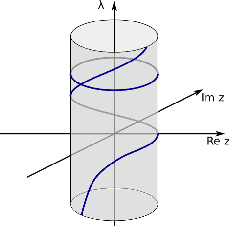
Figure 1. Spectrum of a graph as a function of the parameter $z$, which controls the matching condition of the form (32) at one of the vertices of the graph. The figure shows the non-decreasing function $\Lambda(z)$ spiraling upwards and one of the constant branches from the set $\Delta$.

Theorem 6.1.

There exist a bounded from below discrete set $\Delta\in\mathbb{R}$ and a multiple valued function $\Lambda(z)$ (“dispersion relation”) analytic in a neighborhood of the unit circle $S^{1}$ and real on $S^{1}$, such that:

1. For any $z\in S^{1}$, one has

   (33) $$\sigma(\mathcal{H}(z))=\Lambda(z)\bigcup\Delta,$$

   where $\sigma(A)$ denotes the spectrum of the operator $A$.

2. The function $\Lambda$ is irreducible, i.e. any of its branches determines by analytic continuation the whole function $\Lambda$.

3. Each analytic branch of $\Lambda$ is monotonically increasing in the counter-clockwise direction of $S^{1}$.

Proof.

Notice that, as we already know, for each $z\in S^{1}$, $\mathcal{H}(z)$ is a bounded from below self-adjoint operator with a discrete spectrum. Let $\lambda_{n}(z)$ be its $n$th eigenvalue, counted with multiplicity in non-decreasing order. Then, according to the perturbation theory, it is continuous on the unit circle cut at $z=-1$, where one can observe that the ground state $\lambda_{1}$ has an one-side limit equal to $-\infty$.

Lemma 6.2.

1. The function $\lambda_{n}(z)$ is non-decreasing in the counter-clockwise direction on the unit circle.

2. There exists a function $F(\lambda,z)$ analytic in a neighborhood of the unit circle $S^{1}$ such that $\lambda\in\sigma(\mathcal{H}(z))$ if and only if $F(\lambda,z)=0$.

Indeed, the first claim of the Lemma is a rephrasing of a part of Theorem 5.1 (and, essentially, a consequence of monotonicity of the quadratic form (16) with respect to $\alpha$). The second claim is a direct consequence of Theorem 3.8.

Lemma 6.3.

If either

1. $\lambda$ is a multiple eigenvalue of $\mathcal{H}(z)$, for some $z\in S^{1}$, or

2. $\lambda$ belongs to the spectra of $\mathcal{H}(z_{1})$ and $\mathcal{H}(z_{2})$ for two different points $z_{1},z_{2}\in S^{1}$,

then $\lambda\in\sigma(\mathcal{H}(z))$ for any $z\in S^{1}$.

Indeed, if the eigenspace of $\mathcal{H}(z)$ corresponding to $\lambda$ is more than one-dimensional, then it contains an eigenfunction vanishing at the vertex $v$. Then, assuming $z\neq-1$, we conclude from (32) that the sum of derivatives is zero as well. Therefore this eigenfunction works for any point $z\in S^{1}$. In the case $z=-1$ we select an eigenfunction with vanishing sum of derivatives at $v$ and it automatically vanishes at $v$ since it satisfies the Dirichlet condition.

Let now $\lambda\in\sigma(\mathcal{H}(z_{1}))\bigcap\sigma(\mathcal{H}(z_{2}))$ with the corresponding eigenfunctions $f_{1}$ and $f_{2}$. Without loss of generality, $z_{1}\neq-1$. First consider the case $f_{1}(v)\neq 0$. Then, by Theorem 5.1, $\lambda$ as an eigenvalue of $\mathcal{H}(z_{1})$ lies strictly between consecutive eigenvalues of $\mathcal{H}(z_{2})$ which contradicts our assumption. Thus $f_{1}(v)=0$ and the sum of derivatives of $f_{1}$ is zero by (32). We conclude that $f_{1}$ is an eigenfunction for any $z\in S^{1}$ thus completing the proof of the Lemma.

We now define the set $\Delta$ as the set of all $\lambda\in\mathbb{R}$ such that $\lambda\in\sigma(\mathcal{H}(z))$ for all $z\in S^{1}$. As the previous lemma shows, one can describe $\Delta$ as the intersection $\sigma(\mathcal{H}(-1))\bigcap\sigma(\mathcal{H}(1))$ of the Dirichlet and Neumann spectra and thus is discrete and bounded from below.

Consider now a neighborhood $U$ in $\mathbb{C}$ of the circle $S^{1}$ and the set $\overline{\Sigma}$ that is the closure of the set

(34) $$\Sigma:=\left(\bigcup\limits_{z\in U}\Big{(}\{z\}\times\sigma(\mathcal{H}(z))\Big{)}\right)\setminus\left(\mathbb{C}\times\Delta\right).$$

To put things simply, we remove from the union of the spectra all “horizontal” branches $(z,\lambda)$ with $\lambda\in\Delta$. The second statement of Lemma 6.2 then implies that the set $\overline{\Sigma}$ is analytic. Moreover, for the neighborhood $U$ being sufficiently small, it is a smooth complex analytic curve. Indeed, Lemma 6.3 implies that for all $\lambda\notin\Delta$ the eigenvalues are simple, and thus the eigenvalue branch is analytic. Let now $\lambda\in\Delta$ and $(z_{0},\lambda)\in\overline{\Sigma}$ for some $z_{0}\in S^{1}$. Then Lemma 6.3 says that the eigenvalue $\lambda$ near $z_{0}$ either stays constant, or splits into the constant and possibly one or more increasing branches. The constant branches are excluded in the definition of $\overline{\Sigma}$, equation (34). Also, there can be no more than one increasing branch, otherwise one would find two values of $z$ with the same values of $\lambda$ in $\overline{\Sigma}$, which the lemma allows only to happen on horizontal branches. Moreover, as we have already concluded, the eigenvalue on such a branch must be simple. Then Rellich’s theorem (e.g., [25, v.4, Theorem XII.3]) says that the increasing branch is analytic. We thus conclude that $\overline{\Sigma}$ consists of one or more non-intersecting analytic curves.

We will show now that there is only one component, if the neighborhood $U$ is sufficiently small. First of all, the projection onto the $\lambda$-axis of $S_{j}\bigcap(S^{1}\times\mathbb{R})$, where $S_{j}$ is any of the components of $\overline{\Sigma}$ is the whole real axis, otherwise the component whose projection does not cover the whole real axis would create an accumulation that would contradict the discreteness of the spectrum for each $z\in S^{1}$. Then existence of two or more components would create equal eigenvalues for at least two distinct values of $z$, which would contradict to the Lemma 6.3.

Thus, $\overline{\Sigma}$ is an irreducible analytic curve that intersects each line $\{z\}\times\mathbb{R}$ on the cylinder along the discrete spectrum $\sigma(\mathcal{H}(z))$ and such that it is monotonically increasing counterclockwise. Hence, it forms a kind of a spiral winding around the cylinder infinitely many times when $\lambda\to\infty$ and having a vertical asymptote when $\lambda\to-\infty$ (otherwise one would get a contradiction with the boundedness of each of the spectra from below). This proves the statement of the theorem. ∎

6.2. Nodal count on trees

Here we present a simple proof of a result that was first discovered in [1, 23, 26]. With all ground-setting work done in Section 5 the proof is significantly shortened.

Theorem 6.4.

Let $\lambda_{n}$ be a simple eigenvalue of $-\frac{d^{2}}{dx^{2}}+V(x)$ on a tree graph $\Gamma$ and its eigenfunction $f^{(n)}$ be non-zero at all vertices of $\Gamma$. Then $f^{(n)}$ has $n-1$ zeros on $\Gamma$.

Proof.

To simplify notation we will drop the script $n$ when talking about the eigen-pair $(\lambda_{n},f^{(n)})$. We will prove the result by induction on the number of internal vertices of the tree $\Gamma$. If there are no internal vertices, $\Gamma$ is simply an interval and the statement reduces to the classical Sturm’s Oscillation Theorem (see, e.g. [5]).

Let $v$ be a vertex of degree $d_{v}$. Then $v$ separates $\Gamma$ into $d_{v}$ sub-trees $\Gamma_{i}$, each with a strictly smaller number of internal vertices. For each subtree, the vertex $v$ is a vertex of degree 1 with, so far, no vertex condition. We will impose $\delta$-type condition with the parameter $\alpha_{i}<\infty$ chosen in such a way that the function $f$ restricted to $\Gamma_{i}$ is still an eigenfunction. This value is simply $\alpha_{i}=f_{i}^{\prime}(v)/f_{i}(v)$. The eigenfunction $f$ still corresponds to the eigenvalue $\lambda_{n}$ which is still simple (otherwise we can construct another eigenfunction for the entire tree $\Gamma$, contradicting the simplicity of $\lambda$). It is an $n_{i}$-th eigenvalue of $\Gamma_{i}$ and, applying the inductive hypothesis, we conclude that the function $f$ has $n_{i}-1$ zeros on the subtree $\Gamma_{i}$. Thus we need to understand the relationship between the numbers $n_{i}$ and the number $n$.

To do it, consider the subtree $\Gamma_{i,\infty}$ which now has Dirichlet condition on the vertex $v$. By Theorem 5.1, there are exactly $n_{i}-1$ eigenvalues of $\Gamma_{i,\infty}$ that are smaller than $\lambda$. Now consider the tree $\Gamma_{\infty}$, which is the original tree but with the Dirichlet condition at the vertex $v$. On one hand it has exactly $n-1$ eigenvalues that are smaller than $\lambda$. On the other hand $\Gamma_{\infty}$ is just a disjoint collection of subtrees $\Gamma_{i,\infty}$ and its spectrum is the superposition of the spectra of $\Gamma_{i,\infty}$. Therefore the number of eigenvalues that are smaller than $\lambda$ is

$$n-1=\sum_{i=1}^{d_{v}}(n_{i}-1).$$

Since we already proved that the number of zeros of $f$ is equal to the sum on the right-hand side, we can conclude that $\mu(f)=n-1$. ∎

Appendix A Analytic Fredholm alternative

Here we formulate the following version of the analytic Fredholm alternative:

Theorem A.1.

Let $A(z)$ be an analytic family of Fredholm operators of index zero acting in a Banach space $E$, where $z$ runs over a holomorphically convex domain $\Omega$ in $\mathbb{C}^{n}$ (or a more general Stein analytic manifold). Then there exists an analytic function $f(z)$ in $\Omega$ such that the set of all points $z$ for which $A(z)$ is not invertible coincides with the set of all zeros of the function $f$.

The proof of this statement can be found in many places, e.g. it follows from the Corollary to Theorem 4.11 in [27].

References

- [1] O. Al-Obeid. On the number of the constant sign zones of the eigenfunctions of a dirichlet problem on a network (graph). Technical report, Voronezh: Voronezh State University, 1992. in Russian, deposited in VINITI 13.04.93, N 938 – B 93. – 8 p.
- [2] G. Berkolaiko. A lower bound for nodal count on discrete and metric graphs. Comm. Math. Phys., 278(3):803–819, 2008.
- [3] G. Berkolaiko, R. Carlson, S. Fulling, and P. Kuchment, editors. Quantum graphs and their applications, volume 415 of Contemp. Math., Providence, RI, 2006. Amer. Math. Soc.
- [4] L. Bungart. On analytic fiber bundles. I. Holomorphic fiber bundles with infinite dimensional fibers. Topology, 7:55–68, 1967.
- [5] R. Courant and D. Hilbert. Methods of mathematical physics. Vol. I. Interscience Publishers, Inc., New York, N.Y., 1953.
- [6] D. E. Edmunds and W. D. Evans. Spectral theory and differential operators. Oxford Mathematical Monographs. The Clarendon Press Oxford University Press, New York, 1987. Oxford Science Publications.
- [7] P. Exner, J. P. Keating, P. Kuchment, T. Sunada, and A. Teplyaev, editors. Analysis on graphs and its applications, volume 77 of Proc. Sympos. Pure Math., Providence, RI, 2008. Amer. Math. Soc.
- [8] S. A. Fulling, P. Kuchment, and J. H. Wilson. Index theorems for quantum graphs. J. Phys. A, 40(47):14165–14180, 2007.
- [9] P. R. Garabedian and M. Schiffer. Convexity of domain functionals. J. Analyse Math., 2:281–368, 1953.
- [10] S. Gnutzmann and U. Smilansky. Quantum graphs: Applications to quantum chaos and universal spectral statistics. Adv. Phys., 55(5–6):527–625, 2006.
- [11] P. Grinfeld. Hadamard’s formula inside and out. J. Optim. Theory Appl., 146(3):654–690, 2010.
- [12] J. Hadamard. Mémoire sur le probleme d’analyse relatif a l’equilibre des plaques elastiques encastrees. Mémoires présentés par divers savants l̀’Académie des Sciences, 33, 1908.
- [13] M. Harmer. Hermitian symplectic geometry and extension theory. J. Phys. A, 33(50):9193–9203, 2000.
- [14] L. Ivanov, L. Kotko, and S. Kreĭn. Boundary value problems in variable domains. Differencial′nye Uravnenija i Primenen.—Trudy Sem., 19:1–161, 1977.
- [15] T. Kato. Perturbation theory for linear operators. Classics in Mathematics. Springer-Verlag, Berlin, 1995. Reprint of the 1980 edition.
- [16] V. Kostrykin and R. Schrader. Kirchhoff’s rule for quantum wires. J. Phys. A, 32(4):595–630, 1999.
- [17] P. Kuchment. Graph models for waves in thin structures. Waves Random Media, 12(4):R1–R24, 2002.
- [18] P. Kuchment. Quantum graphs. I. Some basic structures. Waves Random Media, 14(1):S107–S128, 2004. Special section on quantum graphs.
- [19] P. Kuchment. Quantum graphs: an introduction and a brief survey. In Analysis on graphs and its applications, volume 77 of Proc. Sympos. Pure Math., pages 291–312. Amer. Math. Soc., Providence, RI, 2008.
- [20] N. H. Kuiper. The homotopy type of the unitary group of Hilbert space. Topology, 3:19–30, 1965.
- [21] F. Lledó and O. Post. Eigenvalue bracketing for discrete and metric graphs. J. Math. Anal. Appl., 348(2):806–833, 2008.
- [22] J. Peetre. On Hadamard’s variational formula. J. Differential Equations, 36(3):335–346, 1980.
- [23] Y. V. Pokornyĭ, V. L. Pryadiev, and A. Al′-Obeĭd. On the oscillation of the spectrum of a boundary value problem on a graph. Mat. Zametki, 60(3):468–470, 1996.
- [24] O. Post. First order approach and index theorems for discrete and metric graphs. Ann. Henri Poincaré, 10(5):823–866, 2009.
- [25] M. Reed and B. Simon. Methods of modern mathematical physics. I–4. Functional analysis. Academic Press, New York, 1972.
- [26] P. Schapotschnikow. Eigenvalue and nodal properties on quantum graph trees. Waves Random Complex Media, 16(3):167–178, 2006.
- [27] M. G. Zaĭdenberg, S. G. Kreĭn, P. A. Kučment, and A. A. Pankov. Banach bundles and linear operators. Uspehi Mat. Nauk, 30(5(185)):101–157, 1975.