Non-monotoic fluctuation-induced interactions between dielectric slabs carrying charge disorder

Abstract

We investigate the effect of monopolar charge disorder on the classical fluctuation-induced interactions between randomly charged net-neutral dielectric slabs and discuss various generalizations of recent results (A. Naji et al., Phys. Rev. Lett. 104, 060601 (2010)) to highly inhomogeneous dielectric systems with and without statistical disorder correlations. We shall focus on the specific case of two generally dissimilar plane-parallel slabs, which interact across vacuum or an arbitrary intervening dielectric medium. Monopolar charge disorder is considered to be present on the bounding surfaces and/or in the bulk of the slabs, may be in general quenched or annealed and may possess a finite lateral correlation length reflecting possible ‘patchiness’ of the random charge distribution. In the case of quenched disorder, the bulk disorder is shown to give rise to an additive long-range contribution to the total force, which decays as the inverse distance between the slabs and may be attractive or repulsive depending on the dielectric constants of the slabs. By contrast, the force induced by annealed disorder in general combines with the underlying van der Waals forces in a non-additive fashion and the net force decays as an inverse cube law at large separations. We show however that in the case of two dissimilar slabs the net effect due to the interplay between the disorder-induced and the pure van der Waals interactions can lead to a variety of unusual non-monotonic interaction profiles between the dielectric slabs. In particular, when the intervening medium has a larger dielectric constant than the two slabs, we find that the net interaction can become repulsive and exhibit a potential barrier, while the underlying van der Waals force is attractive. On the contrary, when the intervening medium has a dielectric constant in between that of the two slabs, the net interaction can become attractive and exhibit a free energy minimum, while the pure van der Waals force is repulsive. Therefore, the charge disorder, if present, can drastically alter the effective interaction between net-neutral objects.

I Introduction

One of the most persistently made assumptions in the standard theory of (bio)colloid stability is that of a uniform charge distribution on macromolecular surfaces DLVO . There are nevertheless many instances where charge patterns on macromolecular surfaces are inhomogeneous, exhibiting even a highly disordered spatial distribution. Among most notable examples are surfactant-coated surfaces Klein and random polyelectrolytes and polyampholytes rand_polyelec . The macromolecular charge pattern in these systems is often frozen, or quenched, meaning that the charge distribution does not evolve after the assembly or fabrication of the material. This is the case if the interaction between the surface charge carriers and the surfaces is of a chemical nature involving interactions that far exceed the thermal energy scale $k_{\mathrm{B}}T$. Alternatively charge distributions can exhibit various degrees of annealing when interacting with other macromolecules in aqueous solutions as is, for example, the case for charge regulation of contact surfaces bearing weak acidic groups in aqueous solutions ParsegianChan .

Recently it has also been realized that ultrahigh sensitivity experiments on Casimir (zero temperature and ideally polarizable surfaces) and van der Waals (finite temperature and non-ideally polarizable surfaces) interactions between surfaces in vacuo bordag ; kim can be properly understood only if one takes into account the disordered nature of charges on and within the interacting surfaces kim ; speake ; PRL . Possible causes of sample- and history-specific charge disorder in this case include the patch effect, where the variation of the local crystallographic axes of the exposed surface of a clean polycrystalline sample can lead to a variation of the local surface potential barrett . Amorphous films deposited on crystalline substrates can also show a similar type of surface charge disorder, showing a grain structure of dimensions sometimes larger than the thickness of the deposited surface film liu . On the other hand, adsorption of various contaminants can influence the nature and type of the surface charge disorder.

Since the nature and distribution of the charge disorder in any of the force experiments is in general seldom known, we pursue a strategy of assessing the consequences of different a priori models of the distribution of charge disorder. In what follows we will thus assume that the charge disorder stems from randomly distributed monopolar charges which may be present both in the bulk and/or on the interacting surfaces and can be either annealed or quenched. In the quenched case, the disorder charges are frozen, whereas in the annealed case, the disorder charges are subject to thermal fluctuations at ambient temperature and can thus adapt themselves in order to minimize the free energy of the system. We do not deal with effects due to disorder in the dielectric response of the interacting media randomdean , which presents an additional source of disorder meriting further study. We have shown in our previous works ali-rudi ; mama ; PRL that the type and the nature of the charge disorder induces marked changes in the properties of the total interaction between apposed bodies and the force arising from the presence of disordered charges can dominate the underlying Casimir–van der Waals (vdW) effect at sufficiently large separations. The analysis of the interaction fingerprint of the charge disorder can be useful in assessing whether the experimentally observed interactions can be interpreted in terms of disorder effects or are due to pure Casimir–vdW interactions. In this study we will continue with the assessment of this interaction fingerprint in the case two semi-infinite net-neutral dielectric slabs (separated by a layer of vacuum or an arbitrary unstructured dielectric material as shown in Fig. 1), by generalizing our formalism to include two different mechanisms:

1. the “patchy” distribution of the charge disorder, which may arise due to finite correlations between the carriers of the charge disorder. This is a rather realistic assumption in view of the graininess observed in interacting surfaces barrett ; liu .

2. the dielectric inhomogeneity effects in highly asymmetric systems, where the two slabs and the intervening medium may in general have different dielectric properties.

For interacting bodies carrying no net charge, the part of the interaction due to monopolar quenched charge disorder can be seen from a full quantum field-theoretical formalism unpublished to be coupled directly to the zero-frequency or classical vdW interaction (corresponding to the zero-frequency Matsubara modes of the electromagnetic field). The situation would be more complicated in the case of annealed disorder if one is to account for the higher-order Matsubara frequencies and a general treatment is missing at present. In this work, we shall examine the effects of quenched and annealed charge disorder by focusing specifically on the zero-frequency vdW interaction. It is well known that the higher frequency Matsubara terms in the total vdW interaction free energy become relatively unimportant at sufficiently high temperatures and/or sufficiently large intersurface separations bordag . In this paper we will restrict ourselves to this regime which is also most relevant experimentally kim and consider the short-distance quantum effects elsewhere unpublished .

As we shall demonstrate, the interplay and competition of the underlying vdW effect between the two semi-infinite slabs and the interaction induced by the charge disorder can give rise to a variety of different interaction profiles, including, most notably, non-monotonic interactions as a function of the inter-slab distance. In particular, when the two dielectrics interact across a medium of higher dielectric constant, the disorder force can become strongly repulsive and thus generate a potential barrier when combined with the vdW force, which is attractive in that case. While, in the situation where the intervening medium has a dielectric constant in between that of the two slabs vdw_repulsive , the disorder can generate an attractive force, which can balance the repulsive vdW force, leading thus to a stable bound state between the two dielectric slabs. Therefore, the charge disorder, if present, can provide an intrinsic mechanism to stabilize interactions between net-neutral bodies. These features emerge because the disorder-induced interactions typically decay more weakly with the separation than the vdW interaction and depend strongly on the dielectric inhomogeneities in the system.

The above features vary depending on whether the disorder is assumed to be quenched or annealed. The effects due to annealed charge disorder can be distinctly different from those of the quenched charge disorder. In the case of annealed charges, the effective interactions turn out to decay more rapidly and in fact in a similar way as the pure vdW interaction, whereas in the case of quenched charges the net interactions decay more weakly with the separation, i.e., as $\sim D^{-\alpha}$ where $\alpha=1$ if the disorder is present in the bulk of the slabs and $\alpha=2$ if the disorder is confined to the bounding surfaces of the slabs.

The organization of the paper is as follows: In Section II, we introduce the details of our model and the formalism used in our study. The general results are derived in Sections III.1 and III.2 for the case of quenched and annealed disorder, respectively. We shall proceed with the analysis of the effective interaction between two identical slabs in Section IV, where we shall focus mainly on the effects due to spatial correlation in the distribution of the charge disorder. In Section V, we study the interaction in dielectrically asymmetric systems by considering two dissimilar dielectric slabs that interact across an arbitrary dielectric medium. The results and limitations of our study are summarized in Section VI.

II Model

Let us consider two semi-infinite slabs of dielectric constants $\varepsilon_{1}$ and $\varepsilon_{2}$ and temperature $T$ with parallel planar inner surfaces (of infinite area $S$) located normal to the $z$ axis at $z=\pm D/2$ (see Fig. 1). The inner gap is filled with a material of dielectric constant $\varepsilon_{m}$. The inhomogeneous dielectric constant profile for this system is thus given by

$$\varepsilon({\mathbf{r}}) = \left\{\begin{array}[]{ll}\varepsilon_{1}&\quad z<-D/2,\\ \varepsilon_{m}&\quad|z|<D/2,\\ \varepsilon_{2}&\quad z>D/2.\end{array}\right.$$ (4)

We shall assume that the two dielectric slabs have a disordered monopolar charge distribution, $\rho(\mathbf{r})$, which may arise from randomly distributed charges residing on the bounding surfaces [$\rho_{s}(\mathbf{r})$] and/or in the bulk [$\rho_{b}(\mathbf{r})$], i.e., $\rho(\mathbf{r})=\rho_{s}(\mathbf{r})+\rho_{b}(\mathbf{r})$. The charge disorder is assumed to be distributed according to a Gaussian weight with zero mean (i.e., the slabs are net neutral), and the two-point correlation function

$$\langle\!\langle\rho(\mathbf{r})\rho(\mathbf{r}^{\prime})\rangle\!\rangle={\mathcal{G}}({\bm{\varrho}}-{\bm{\varrho}}^{\prime};z)\delta(z-z^{\prime}),$$ (5)

where $\langle\!\langle\cdots\rangle\!\rangle$ denotes the average over all realizations of the charge disorder distribution, $\rho(\mathbf{r})$. We have thus assumed that there are no spatial correlations in the perpendicular direction, $z$, while, in the lateral directions ${\bm{\varrho}}=(x,y)$ (in the plane of the dielectrics), we have a finite statistically invariant correlation function whose specific form may depend on $z$ as well. This implies that the charge disorder is distributed in general as random “patches” in a layered structure in the bulk of the slabs as well as on the bounding surfaces.

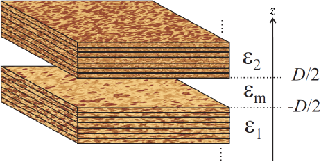
Figure 1: (Color online) We consider two semi-infinite net-neutral slabs (half-spaces) of dielectric constant $\varepsilon_{1}$ and $\varepsilon_{2}$ interacting across a medium of dielectric constant $\varepsilon_{m}$. The monopolar charge disorder (shown schematically by small light and dark patches) is distributed as random patches of finite typical size (correlation length) in a layered structure in the bulk of the slabs and on the two bounding surfaces at $z=\pm D/2$. It may be either quenched or annealed.

The total correlation function can be written as the sum of the surface ($s$) and bulk ($b$) contributions

$${\mathcal{G}}({\bm{\varrho}}-{\bm{\varrho}}^{\prime};z)=g_{s}(z)c_{s}({\bm{\varrho}}-{\bm{\varrho}}^{\prime};z)+g_{b}(z)c_{b}({\bm{\varrho}}-{\bm{\varrho}}^{\prime};z).$$ (6)

For the slab geometry, we generally assume that the lateral correlation functions may be different for the two slabs, i.e.

$$c_{s}({\mathbf{x}};z) = \left\{\begin{array}[]{ll}c_{1s}({\mathbf{x}})&\quad z=-D/2,\\ c_{2s}({\mathbf{x}})&\quad z=D/2,\end{array}\right.$$ (9)

$$c_{b}({\mathbf{x}};z) = \left\{\begin{array}[]{ll}c_{1b}({\mathbf{x}})&\quad z<-D/2,\\ 0&\quad|z|<D/2,\\ c_{2b}({\mathbf{x}})&\quad z>D/2,\end{array}\right.$$ (13)

and that the surface and bulk variances are given by

$$g_{s}(z) = e_{0}^{2}[g_{1s}\delta(z+D/2)+g_{2s}\delta(z-D/2)],$$ (14)

$$g_{b}(z) = \left\{\begin{array}[]{ll}g_{1b}e_{0}^{2}&\quad z<-D/2,\\ 0&\quad|z|<D/2,\\ g_{2b}e_{0}^{2}&\quad z>D/2.\end{array}\right.$$ (18)

The lateral correlation between two given points is typically expected to decay with their separation over a finite correlation length (“patch size”), which could in general be highly material or sample specific. However, the main aspects of the patchy structure of the disorder can be investigated by assuming simple generic models with, for instance, a Gaussian or an exponentially decaying correlation function. Without loss of generality, we shall choose an exponentially decaying correlation function according to the two-dimensional Yukawa form

$$c_{i\alpha}({\mathbf{x}})=\frac{1}{2\pi\xi_{i\alpha}^{2}}\,\mathrm{K}_{0}\!\left(\frac{|{\mathbf{x}}|}{\xi_{i\alpha}}\right),$$ (19)

where $\xi_{i\alpha}$ represents the correlation length for the bulk or surface disorder ($\alpha=b,s$) in the $i$-th slab ($i=1,2$). The case of a completely uncorrelated disorder PRL follows as a special case for $\xi_{i\alpha}\rightarrow 0$ from our formalism. We should emphasize that the correlation assumed for the bulk disorder is only present in the plane of the slab surfaces and not in the direction perpendicular to them. This assumption is wholly justified only for layered materials. In all the other cases of the bulk disorder one would normally expect the same correlation length in the direction perpendicular to the surfaces. We will deal with this model in a separate publication.

III Formalism

The partition function for the classical vdW interaction (the zero-frequency Matsubara modes of the electromagnetic field) may be written as a functional integral over the scalar field $\phi(\mathbf{r})$,

$${\mathcal{Z}}[\rho(\mathbf{r})]=\int[{\mathcal{D}}\phi(\mathbf{r})]\,\,e^{-\beta{\mathcal{S}}[\phi(\mathbf{r});\rho(\mathbf{r})]},$$ (20)

with $\beta=1/k_{\mathrm{B}}T$ and the effective action

$${\mathcal{S}}[\phi(\mathbf{r});\rho(\mathbf{r})]=\int{\mathrm{d}}\mathbf{r}\,\big{[}{\textstyle{\frac{1}{2}}}\varepsilon_{0}\varepsilon({\mathbf{r}})\,(\nabla\phi(\mathbf{r}))^{2}+{\mathrm{i}}\,\rho(\mathbf{r})\phi(\mathbf{r})\big{]}.$$ (21)

The above partition function can be used to evaluate averaged quantities such as the effective interaction between the dielectric bodies. However, since the charge distribution, $\rho(\mathbf{r})$, is disordered, it is necessary to average the partition function over different realizations of the charge distribution. The averaging procedure differs depending on the nature of the disorder. In what follows, we consider two idealized cases of either completely quenched or completely annealed disorder dotsenko1 (the intermediate case of partially annealed disorder is also analytically tractable mama but will not be considered here).

III.1 Correlated quenched disorder

The quenched disorder corresponds to the situation where the disorder charges are frozen and can not fluctuate and equilibrate with other degrees of freedom in the system. As it is well known, the disorder average in this case must be taken over the sample free energy, $\ln{\mathcal{Z}}[\rho(\mathbf{r})]$, in order to evaluate the averaged quantities dotsenko1 . Therefore, the free energy of the quenched model is given by

$$\beta{\mathcal{F}}_{\mathrm{quenched}}=-\langle\!\langle\ln{\mathcal{Z}}[\rho(\mathbf{r})]\rangle\!\rangle.$$ (22)

The Gaussian integral in Eq. (20) as well as the disorder average can be evaluated straightforwardly in this case yielding

$$\beta{\mathcal{F}}_{\mathrm{quenched}} = {\textstyle{\frac{1}{2}}}{\mathrm{Tr}}\ln G^{-1}({\mathbf{r}},{\mathbf{r}}^{\prime})$$

$$+ {\textstyle{\frac{\beta}{2}}}\int\!{\mathrm{d}}{\mathbf{r}}\,{\mathrm{d}}{\mathbf{r}}^{\prime}\,{\mathcal{G}}({\bm{\varrho}}-{\bm{\varrho}}^{\prime};z)\delta(z-z^{\prime})G({\mathbf{r}},{\mathbf{r}}^{\prime}),$$

where $G({\mathbf{r}},{\mathbf{r}}^{\prime})$ is the Green’s function defined via

$$\varepsilon_{0}\nabla\cdot[\varepsilon(\mathbf{r})\nabla G(\mathbf{r},\mathbf{r}^{\prime})]=-\delta(\mathbf{r}-\mathbf{r}^{\prime}).$$ (24)

Note that the free energy (III.1) of the quenched model is expressed in terms of different additive contributions, i.e.

$${\mathcal{F}}_{\mathrm{quenched}}={\mathcal{F}}_{\mathrm{vdW}}+{\mathcal{F}}_{b}+{\mathcal{F}}_{s}.$$ (25)

The first term above is nothing but the usual contribution from the zero-frequency vdW interaction,

$$\beta{\mathcal{F}}_{\mathrm{vdW}}={\textstyle{\frac{1}{2}}}{\mathrm{Tr}}\ln G^{-1}({\mathbf{r}},{\mathbf{r}}^{\prime}),$$ (26)

which is always present between neutral dielectrics even in the absence of any monopolar charge disorder. The second and the third terms represent contributions from the bulk and surface disorder ($\alpha=b,s$)

$$\beta{\mathcal{F}}_{\alpha}={\textstyle{\frac{\beta}{2}}}\int\!{\mathrm{d}}{\mathbf{r}}\,{\mathrm{d}}{\mathbf{r}}^{\prime}\,g_{\alpha}(z)c_{\alpha}({\bm{\varrho}}-{\bm{\varrho}}^{\prime};z)\delta(z-z^{\prime})G({\mathbf{r}},{\mathbf{r}}^{\prime}).$$ (27)

The quenched expression (III.1) is valid for any arbitrary disorder correlation function ${\mathcal{G}}({\bm{\varrho}}-{\bm{\varrho}}^{\prime};z)$ and dielectric constant profile $\varepsilon({\mathbf{r}})$. In what follows, we shall focus on the particular case of planar dielectrics by employing Eqs. (4), (6)-(18). In this case, the zero-frequency vdW contribution is obtained (per $k_{\mathrm{B}}T$ and unit area) as bordag

$$\frac{\beta{\mathcal{F}}_{\mathrm{vdW}}}{S}={\frac{1}{2}}\!\int\!\!\frac{{\mathrm{d}}^{2}Q}{(2\pi)^{2}}\ln{(1-\Delta_{1}\Delta_{2}\,e^{-2QD})}.$$ (28)

The force associated with this contribution, $f_{\text{vdW}}=-\partial{\mathcal{F}}_{\mathrm{\text{vdW}}}/\partial D$, follows as

$$\frac{\beta f_{{\text{vdW}}}}{S}=-\frac{{\mathrm{Li}}_{3}(\Delta_{1}\Delta_{2})}{8\pi D^{3}}.$$ (29)

The dielectric jump parameters are defined as

$$\Delta_{i}=\frac{\varepsilon_{i}-\varepsilon_{m}}{\varepsilon_{i}+\varepsilon_{m}}$$ (30)

at each of the bounding surfaces ($i=1,2$), and ${\mathrm{Li}}_{3}(\cdot)$ is the trilogarithm function defined by

$${\rm Li}_{3}(z)=\sum_{n=1}^{\infty}{z^{n}\over n^{3}}.$$ (31)

The dielectric constants of the system enter the expression (28) via the terms $\Delta_{1}$ and $\Delta_{2}$. If $\Delta_{1}\Delta_{2}>0$ then the vdW interaction between the slabs is attractive, otherwise the vdW force is repulsive.

The expression in Eq. (27) can be calculated in a straightforward manner. We obtain the bulk disorder contribution as

$$\frac{\beta{\mathcal{F}}_{b}}{S} =-\ell_{\mathrm{B}}\varepsilon_{m}\times$$

$$\int\!\frac{{\mathrm{d}}Q}{Q}\frac{e^{-2QD}}{1-\Delta_{1}\Delta_{2}e^{-2QD}}\bigg{[}\!\frac{g_{1b}c_{1b}(Q)}{(\varepsilon_{1}\!+\!\varepsilon_{m})^{2}}\Delta_{2}\!+\!\frac{g_{2b}c_{2b}(Q)}{(\varepsilon_{2}\!+\!\varepsilon_{m})^{2}}\Delta_{1}\!\bigg{]},$$

and the surface disorder contribution as

$$\frac{\beta{\mathcal{F}}_{s}}{S} =-2\ell_{\mathrm{B}}\varepsilon_{m}\times$$

$$\int\!\mathrm{d}Q\frac{e^{-2QD}}{1-\Delta_{1}\Delta_{2}e^{-2QD}}\bigg{[}\!\frac{g_{1s}c_{1s}(Q)}{(\varepsilon_{1}\!+\!\varepsilon_{m})^{2}}\Delta_{2}\!+\!\frac{g_{2s}c_{2s}(Q)}{(\varepsilon_{2}\!+\!\varepsilon_{m})^{2}}\Delta_{1}\!\bigg{]},$$

at all separations $D$, where

$$\ell_{\mathrm{B}}=\beta e_{0}^{2}/(4\pi{\varepsilon_{0}})$$ (34)

is the Bjerrum length in vacuum ($\ell_{\mathrm{B}}\simeq 56.8$ nm at room temperature), and $c_{i\alpha}(Q)$ is the Fourier transform of the correlation function $c_{i\alpha}({\mathbf{x}})$. For the particular form of $c_{i\alpha}({\mathbf{x}})$ chosen in Eq. (19), we have a Lorentzian Fourier transform (for $i=1,2$ and $\alpha=b,s$) as

$$c_{i\alpha}(Q)=\frac{1}{\xi_{i\alpha}^{2}Q^{2}+1}.$$ (35)

The total force between the dielectric slabs carrying quenched charge disorder thus follows from $f_{\mathrm{quenched}}=-\partial{\mathcal{F}}_{\mathrm{quenched}}/\partial D$ and the preceding free energy expressions as

$$\frac{\beta{f}_{\mathrm{quenched}}}{S} = -\frac{{\mathrm{Li}}_{3}(\Delta_{1}\Delta_{2})}{8\pi D^{3}}-2\ell_{\mathrm{B}}\varepsilon_{m}\times$$

$$\!\!\int_{0}^{\infty}\!\!\!\!\!\frac{{\mathrm{d}}Q~{}e^{-2QD}}{\big{(}1\!-\!\Delta_{1}\Delta_{2}e^{-2QD}\big{)}^{2}}\bigg{[}\!\frac{g_{1b}c_{1b}(Q)}{(\varepsilon_{1}\!+\!\varepsilon_{m})^{2}}\Delta_{2}\!+\!\frac{g_{2b}c_{2b}(Q)}{(\varepsilon_{2}\!+\!\varepsilon_{m})^{2}}\Delta_{1}\!+$$

$$\hskip 5.69046pt+\frac{2Qg_{1s}c_{1s}(Q)}{(\varepsilon_{1}\!+\!\varepsilon_{m})^{2}}\Delta_{2}\!+\!\frac{2Qg_{2s}c_{2s}(Q)}{(\varepsilon_{2}\!+\!\varepsilon_{m})^{2}}\Delta_{1}\bigg{]}.$$

We notice that the quenched disorder contribution to the force has a number of interesting features. We see that the forces generated due to the charge disorder in slab 1 and slab 2 are independent and additive. If we remove the charge disorder from either slab we see there is still a contribution coming from the other slab. This is because the charge distributions on average do not interact with each other. As the charge distribution in opposing slabs is uncorrelated, the average force on a charge in slab 1 due to a charge in slab 2 is zero as the charge in slab two is equally likely to have a positive charge as a negative charge. In fact the charges in slab 1 are only correlated with their image charges in slab 2, this means that on average the charge distribution in slab 1 only interacts with its image in slab 2 and vice versa. The sign of the interaction between charges in slab 1 and their images in slab 2 depends on $\Delta_{2}$. If $\Delta_{2}$ is positive, that is the dielectric constant of slab 2 is greater than that of the intervening material, $\varepsilon_{2}>\varepsilon_{m}$, then the force due to the charge in slab 1 is attractive. Therefore, the contribution of the charge in each slab to the net force depends on the dielectric contrast between the opposing slab and the intervening medium. Thus, while the vdW contribution depends on the product $\Delta_{1}\Delta_{2}$, the contribution from the quenched charge distribution in slab 1 depends on variance $g_{1s,b}$ of the charge on the surface or bulk of this slab but on $\Delta_{2}$ of the slab 2. This leads to a rich phenomenology of possible net interactions. For example, if $\Delta_{1}$ and $\Delta_{2}$ are both positive, the vdW force is attractive and so are the forces due to both charge distributions. However, if $\Delta_{1}$ and $\Delta_{2}$ are negative the vdW force is again attractive but the force due to both quenched charge distributions is repulsive. Also, note that while the vdW term shows a standard $1/D^{3}$ decay with the surface separation $D$, the disorder contribution turns out to have a much weaker decay with the separation PRL as we shall analyze further in the forthcoming sections. Therefore, the interplay between these different contributions can lead to characteristically different interaction profiles depending on the system parameters.

III.2 Correlated annealed disorder

In the annealed model, disorder charges are assumed to fluctuate in thermal equilibrium with the rest of the system, and thus in particular the charge distribution in the two slabs can adapt itself to minimize the free energy of the system. In this case, the disorder degrees of freedom should be treated statistically on the same footing as other degrees of freedom, which implies that the disorder average must be taken over the sample partition function ${\mathcal{Z}}[\rho(\mathbf{r})]$ dotsenko1 . Hence, the free energy of the annealed model reads

$$\beta{\mathcal{F}}_{\mathrm{annealed}}=-\ln\,\langle\!\langle{\mathcal{Z}}[\rho(\mathbf{r})]\rangle\!\rangle.$$ (37)

The annealed free energy may be evaluated using Eqs. (5), (20) and (37) as

$$\beta{\mathcal{F}}_{\mathrm{annealed}}={\frac{1}{2}}{\mathrm{Tr}}\ln\big{[}G^{-1}({\mathbf{r}},{\mathbf{r}}^{\prime})+\beta{\mathcal{G}}({\bm{\varrho}}-{\bm{\varrho}}^{\prime};z)\delta(z-z^{\prime})\big{]}.$$ (38)

Note that unlike the quenched case, Eq. (III.1), the disorder contributions cannot be in general separated from the pure vdW contribution when the disorder is annealed.

In the case of two interacting planar dielectrics, we shall make use of Eqs. (4) and (6)-(18) in order to calculate the fluctuational trace-log of the modified inverse Green’s function $G^{-1}({\mathbf{r}},{\mathbf{r}}^{\prime})+\beta{\mathcal{G}}({\bm{\varrho}}-{\bm{\varrho}}^{\prime};z)\delta(z-z^{\prime})$ in Eq. (38). By employing standard procedures rudi_jcp , we find

$$\frac{\beta{\mathcal{F}}_{\mathrm{annealed}}}{S}={\frac{1}{2}}\int\frac{{\mathrm{d}}^{2}Q}{(2\pi)^{2}}\ln\big{[}1-\Delta_{1g}(Q)\Delta_{2g}(Q)e^{-2QD}\big{]},$$ (39)

where we have (for $i=1,2$)

$$\Delta_{ig}(Q) =$$

$$=\frac{\varepsilon_{m}Q\!-\!\varepsilon_{i}\sqrt{Q^{2}\!+\!4\pi\ell_{\mathrm{B}}g_{ib}~{}c_{ib}(Q)/\varepsilon_{i}}\!-\!4\pi\ell_{\mathrm{B}}g_{is}~{}\!c_{is}(Q)}{\varepsilon_{m}Q\!+\!\varepsilon_{i}\sqrt{Q^{2}\!+\!4\pi\ell_{\mathrm{B}}g_{ib}~{}c_{ib}(Q)/\varepsilon_{i}}+4\pi\ell_{\mathrm{B}}g_{is}~{}\!c_{is}(Q)}.$$

The total force, $f_{\mathrm{annealed}}=-\partial{\mathcal{F}}_{\mathrm{annealed}}/\partial D$, in the annealed model thus follows as

$$\frac{\beta{f}_{\mathrm{annealed}}}{S}=-\frac{1}{2\pi}\!\int Q^{2}{\mathrm{d}}Q\frac{\Delta_{1g}(Q)\Delta_{2g}(Q)\,e^{-2QD}}{1-\Delta_{1g}(Q)\Delta_{2g}(Q)\,e^{-2QD}}.$$ (41)

The annealed interaction free energy, or the corresponding force, has a form reminiscent of the zero-frequency vdW interaction between two semi-infinite slabs ninham with renormalized dielectric missmatch, $\Delta_{ig}(Q)$, depending on the in-plane wave-vector $Q$. Indeed, one can argue for the following exact correspondence based on the vdW interactions between media with volume and surface embedded mobile charges ninham ; rudiold : the term $\sqrt{Q^{2}\!+\!4\pi\ell_{\mathrm{B}}g_{ib}~{}c_{ib}(Q)/\varepsilon_{i}}$ corresponds to bulk Debye-like “screening”, stemming from the annealed bulk disorder response to local electrostatic fields. It can be obtained alternatively by analyzing the fluctuational modes of the Debye-Hückel fields as opposed to the Laplace fields ninham . The term $4\pi\ell_{\mathrm{B}}g_{is}~{}\!c_{is}(Q)$, on the other hand, stemms from the response of the mobile charges confined to the dielectric surfaces to electrostatic fields, corresponding to surface disorder-generated “screening” rudiold . It can be derived alternatively by considering the response of the surface polarization to local electrostatic fileds rudiold . The combination of the two terms in Eq. (III.2) can not be written as a sum of two terms depending linearly on $c_{ib}$ and $c_{is}$. This signifies that the bulk and surface disorder effects for the annealed case are obviously not additive and can not be analyzed separately.

Figure 2: a) Magnitude of the rescaled total force, $\beta|f|l_{\mathrm{B}}^{3}/S$ (Eq. (III.1)), between two identical net-neutral dielectric slabs in vacuum ($\varepsilon_{m}=1$) bearing quenched monopolar charge disorder as a function of the rescaled distance, $D/l_{\mathrm{B}}$. The results are plotted here for fixed $\varepsilon_{p}=10$, $g_{s}=0$ (no surface disorder) and bulk disorder variance $g_{b}=5\times 10^{-8}\,{\mathrm{nm}}^{-3}$ and varying disorder correlation length $\xi/l_{\mathrm{B}}=0,200,10^{3},10^{4},10^{5}$ (from top to bottom). Inset shows the ratio of the total force to the pure zero-frequency vdW force (45) between the slabs in the absence of charge disorder for the same range of $D$. b) Same as (a) but here we fix $\varepsilon_{p}=10$, $g_{s}=0$, $\xi/l_{\mathrm{B}}=200$ and vary the bulk disorder variance in the range $g_{b}=10^{-7},10^{-8},10^{-9},10^{-10},10^{-11}\,{\mathrm{nm}}^{-3}$ (from top to bottom). Solid curve is the pure vdW force (45). c) Same as (b) but here we fix $\xi/l_{\mathrm{B}}=200$, $g_{b}=5\times 10^{-8}\,{\mathrm{nm}}^{-3}$, $g_{s}=g_{b}^{2/3}$ and vary the dielectric constant of slabs as $\varepsilon_{p}=2$ (top dotted curve), 10, 40, 100 (bottom dot-dashed curve). All graphs are plotted in log-log scale.

IV Symmetric case of two identical slabs

We now analyze the preceding analytical results in the situation where the two dielectric slabs are identical, i.e., we have $\varepsilon_{i}=\varepsilon_{p}$ ($\Delta_{i}=\Delta$), $g_{is}=g_{s}$, $g_{ib}=g_{b}$, and $\xi_{is}=\xi_{ib}=\xi$ for both slabs $i=1,2$.

IV.1 Quenched disorder-induced interactions

In the case of quenched disorder, one can expand the Lorentzian correlation function $c_{i\alpha}(Q)$, Eq. (35), in powers of the dimensionless ratio of the correlation length to the intersurface separation, $\xi/D$, and thus express the total force (III.1) in the form of a series expansion as

$$f_{\mathrm{quenched}}=f^{(0)}+\sum_{n=1}^{\infty}f^{(n)},$$ (42)

where we have

$$\frac{\beta{f}^{(0)}}{S}=-\frac{g_{b}\ell_{\mathrm{B}}\Delta}{2\varepsilon_{p}D}-\frac{2\varepsilon_{m}g_{s}\ell_{\mathrm{B}}\ln(|1-\Delta^{2}|)}{(\varepsilon_{m}+\varepsilon_{p})^{2}\Delta\,D^{2}}-\frac{{\mathrm{Li}}_{3}(\Delta^{2})}{8\pi D^{3}},$$ (43)

corresponding to the free energy of the system in the presence of a completely uncorrelated disorder ($\xi=0$), and

$$\frac{\beta{f}^{(n)}}{S}=\! - \!\frac{4g_{b}\ell_{\mathrm{B}}\varepsilon_{m}}{(\varepsilon_{m}+\varepsilon_{p})^{2}\Delta D}\!\sum_{n=1}^{\infty}(-1)^{n}\frac{\xi^{2n}}{D^{2n}}C_{2n+1}\mathrm{Li}_{2n}(\Delta^{2})$$ (44)

$$-\frac{8g_{s}\ell_{\mathrm{B}}\varepsilon_{m}}{(\varepsilon_{m}+\varepsilon_{p})^{2}\Delta D^{2}}\!\sum_{n=1}^{\infty}(-1)^{n}\frac{\xi^{2n}}{D^{2n}}C_{2n+2}\mathrm{Li}_{2n+1}(\Delta^{2}),$$

with $C_{n}=\Gamma(n)/2^{n}$. The above series expansion is most suitable for the situation where $\xi/D$ is small.

Let us first consider the leading-order uncorrelated disorder free energy ${f}^{(0)}$ in Eq. (43). This contribution exhibits a few remarkable features PRL . First, it shows a sequence of scaling behaviors with the separation that stem from different origins: a leading $1/D$ term due to the quenched bulk disorder, a subleading $1/D^{2}$ term from the surface charge disorder, and the pure vdW term that goes as $1/D^{3}$, i.e.

$$\frac{\beta f_{{\text{vdW}}}}{S}=-\frac{{\mathrm{Li}}_{3}(\Delta^{2})}{8\pi D^{3}}.$$ (45)

While the vdW term is always attractive in a symmetric system, the disorder contributions (first and second terms in Eq. (43)) are attractive when the dielectric mismatch $\Delta>0$ (i.e., when the dielectric constant of the intervening medium is smaller than that of the slabs) and repulsive otherwise. The former case ($\Delta>0$) has been investigated in detail previously in the context of two identical dielectric slabs in vacuum ($\varepsilon_{m}=1$) PRL .

Note that since the forces induced by an uncorrelated disorder exhibit a much weaker decay with the separation, they may completely mask the standard vdW force (which is always present regardless of any charge disorder) at sufficiently large separations PRL . One might expect that globally electroneutral slabs would exhibit a dipolar-like interaction force to the leading order rather than the monopolar forms $1/D$ (or $1/D^{2}$) obtained for the bulk (or surface) charge distribution. As noted before, the physics involved is indeed subtle as the disorder terms result from the self-interaction of the charges with their images (which follows from $G({\mathbf{r}},{\mathbf{r}})$, Eq. (III.1), in the limit of zero correlation length) and not from dipolar interactions (which come from an expansion of $G({\mathbf{r}},{\mathbf{r}}^{\prime})$ when $|{\mathbf{r}}-{\mathbf{r}}^{\prime}|$ is large). Statistically speaking each charge on average (as any other charge has an equal probability of being of the same or opposite sign) only sees its image, thus explaining the leading monopolar form in the net force.

The next leading correction due to disorder correlations for small $\xi/D$ follows from Eq. (44) as

$$\frac{\beta{f}^{(1)}}{S}\simeq\frac{g_{b}\ell_{\mathrm{B}}\varepsilon_{m}\xi^{2}\Delta\,\mathrm{Li}_{2}(\Delta^{2})}{(\varepsilon_{p}+\varepsilon_{m})^{2}D^{3}}+\frac{3\varepsilon_{m}g_{s}\ell_{\mathrm{B}}\xi^{2}\,\mathrm{Li}_{3}(\Delta^{2})}{(\varepsilon_{m}+\varepsilon_{p})^{2}\Delta\,D^{4}},$$ (46)

which has an opposite sign to the zeroth-order term, and thus tends to weaken the zeroth-order effect. Note however that the higher-order corrections in Eq. (44) alternatively change sign and their net effect leads to a total force which can be evaluated numerically, e.g., directly from Eq. (III.1). The results are shown in Fig. 2 for the case of two identical dielectric slabs in vacuum. As seen in Fig. 2a, the attractive disorder-inducd forces indeed diminish (albeit rather slowly as seen in the inset) as the disorder correlation length is increased (by several orders of magnitude from $\xi=0$ up to $\xi\simeq 5$mm in actual units in the figure). For a large correlation length or at small separation (large $\xi/D$), the total force thus tends to the non-disoredred vdW force (45) that scales as $1/D^{3}$ (thick solid line), while for a small correlation length or at large separation (small $\xi/D$), the force increases and shows a crossover to the maximal uncorrelated disorder value (43) that scales as $1/D$ (top dotted line). The latter is obviously from the bulk disorder which, if present, gives rise to the most dominant effects.

The crossover behavior depends also significantly on the disorder variance and the dielectric mismatch (Figs. 2b and c). Similar trends as described above can be observed by varying the bulk disorder variance, $g_{b}$, as shown in Fig. 2b (here $g_{b}$ varies within the typical range $10^{-11}-10^{-7}\,{\mathrm{nm}}^{-3}$ corresponding to impurity charge densities of $10^{10}-10^{14}\,e_{0}/{\mathrm{cm}}^{3}$ Kao_Pitaevskii ). The results in Fig. 2c however reveal a nonmonotonic dependence on the dielectric mismatch: The disorder contribution tends to decrease both for small and large slab dielectric constant. This can be seen directly from Eqs. (43) and (44) as the disorder-induced force vanishes in the limits $\varepsilon_{p}\rightarrow\infty$ or $\Delta\rightarrow 1$ (perfect conductor) and $\Delta\rightarrow 0$ (homogeneous medium, in which case the vdW force vanishes as well).

It is interesting to note that the first-order corrections due to bulk correlations scales as $1/D^{3}$, which is similar to the vdW contribution. Hence, these corrections tend to renormalize the ideal zero-frequency Hamaker coefficient, $A\equiv 3(k_{\mathrm{B}}T){\mathrm{Li}}_{3}(\Delta^{2})/4$, associated with the vdW term (defined via $f_{\mathrm{vdW}}/S=-A/(6\pi D^{3})$) to an effective value given by

$$A_{\mathrm{eff}}=\frac{3k_{\mathrm{B}}T}{4}{\mathrm{Li}}_{3}(\Delta^{2})+\frac{3g_{b}e_{0}^{2}\,\varepsilon_{m}\Delta\xi^{2}\mathrm{Li}_{2}(\Delta^{2})}{2\varepsilon_{0}(\varepsilon_{p}+\varepsilon_{m})^{2}}.$$ (47)

This value is larger (smaller) than the ideal value $A$ when $\Delta>0$ ($\Delta<0$) and can even change sign.

Figure 3: a) Ratio of the total force (41) to the zero-frequency vdW force (45) between two identical net-neutral dielectric slabs in vacuum ($\varepsilon_{m}=1$) bearing annealed monopolar charge disorder as a function of the rescaled distance, $D/l_{\mathrm{B}}$. The results are plotted here for fixed $\varepsilon_{p}=10$, $g_{s}=0$ (no surface disorder), $g_{b}=5\times 10^{-8}\,{\mathrm{nm}}^{-3}$ and varying disorder correlation length $\xi/l_{\mathrm{B}}=0,200,10^{3},10^{4}$ (from top to bottom). Annealed curves are bounded by the perfect conductor result, Eq. (48) (top solid line), for large disorder and the vdW result, Eq. (45) (bottom solid line), for no disorder. b) Same as (a) but here we have fixed $\varepsilon_{p}=10$, $g_{s}=0$, $\xi/l_{\mathrm{B}}=200$ and bulk disorder variance varied in the range $g_{b}=10^{-7},10^{-8},10^{-9},10^{-10},10^{-11}\,{\mathrm{nm}}^{-3}$ (from top to bottom). c) Same as (a) but here we fix $g_{s}=0$, $g_{b}=5\times 10^{-8}\,{\mathrm{nm}}^{-3},\xi=0$, and vary the dielectric constant of the slabs as $\varepsilon_{p}=2,10,40,100$ (from top). Inset shows a closer view of the curves for $\varepsilon_{p}=40,100$ (from top). Top dotted lines correspond to Eq. (48). All graphs are plotted in log-log scale.

IV.2 Annealed disorder-induced interactions

In the case of annealed disorder, the total force between the dielectric slabs is given by Eq. (41). It shows that the force in this case cannot be expressed simply as a sum of different additive contributions as in the quenched case. Rather, it follows from the combined effect of the annealed disorder fluctuations and the underlying vdW effect, which again reflects the fact that the disorder charge distribution in this case can adapt itself in order to minimize the total free energy of the system.

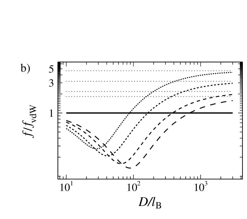
Figure 4: a) Same as Fig. 3a but here we fix $\varepsilon_{p}=50$, $g_{s}=0$, $g_{b}=5\times 10^{-8}\,{\mathrm{nm}}^{-3}$, $\xi=0$, and vary the dielectric constant of the intervening medium as $\varepsilon_{m}=2,10,20,40$ (from bottom to top). b) Same as (a) but here we fix the dielectric constant of the slab as $\varepsilon_{p}=10$ and vary that of the intervening medium as $\varepsilon_{m}=30,40,60,80$ (from top to bottom). Top dotted lines correspond to Eq. (48).

The resulting total force is shown in Fig. 3 for the symmetric case of two identical dielectric slabs in vacuum. For the sake of presentation, we have plotted the ratio of the annealed force (41) to the vdW force (45), which clearly shows that the net force is bounded by two limiting laws, namely, the ideal limiting force

$$\frac{\beta f_{\mathrm{ideal}}}{S}=-\frac{\zeta(3)}{8\pi D^{3}},$$ (48)

which is similar to the one obtained between perfect conductors bordag , and the vdW force (45) in the absence of any disorder charges. These constitute the upper and the lower bounds for the annealed force in the general symmetric case with $\Delta>0$, i.e.

$$|f_{\mathrm{vdW}}|<|f_{\mathrm{annealed}}|<|f_{\mathrm{ideal}}|.$$ (49)

Note that the above limiting values can be established systematically from the general expression (41), and are strictly attractive (negative sign). The lower bound vdW force is non-universal (i.e., material dependent) and is obtained asymptotically in the limit of small disorder variance ($g_{b}$, $g_{s}\rightarrow 0$) or small separationss. The upper bound is universal and follows in the limit of strong disorder variance ($g_{b}$ or $g_{s}\rightarrow\infty$) or large separations. The crossover from one limit to the other can be achieved by increasing the distance or the disorder variance as seen in Fig. 3.

In the annealed case, the disorder correlations play a similar role as in the quenched case and tend to weaken the disorder-induced forces. As seen in Fig. 3a, the magnitude of the force drops from its value for an uncorrelated disorder ($\xi=0$), and also the crossover between the two limiting behaviors as discussed above is ‘delayed’ when the disorder has a finite correlation length, $\xi$.

Figure 5: The rescaled magnitude of the (attractive) force, Eq. (41), between two identical net-neutral dielectric slabs bearing annealed monopolar charge disorder in a dielectrically homogeneous system ($\varepsilon_{1}=\varepsilon_{2}=\varepsilon_{m}$) as a function of the rescaled distance, $D/l_{\mathrm{B}}$. Here we plot the resulting force for $\varepsilon_{1}=\varepsilon_{2}=\varepsilon_{m}=1,10,40,100$ (from top to bottom) and for uncorrelated bulk disorder in both slabs with $\xi=0$, $g_{b}=5\times 10^{-8}\,{\mathrm{nm}}^{-3}$ and $g_{s}=0$. Top solid line shows the universal limiting expression (48).

It is also remarkable to note that Eq. (48) is obtained in general as the large-distance ($D\rightarrow\infty$) behavior for the total force between any two arbitrary dielectric slabs regardless of their dielectric constant and disorder variance. It thus demonstrates the intuitive fact that dielectric slabs with annealed charges tend to behave asymptotically in a way similar to perfect conductors. This is one of the distinctive features of the annealed disorder as compared with the quenched disorder, whose effects depend significantly on the material properties. The deviations due to material properties and the disorder variance in the annealed case contribute a repulsive subleading force in the symmetric case, which can be determined from a series expansion at large separations. If the surface disorder is negligible as compared with the bulk disorder ($g_{s}\ll g_{b}\ell_{\mathrm{B}}$), we obtain (up to the first few leading orders)

$$\frac{\beta f_{\mathrm{annealed}}}{S}\simeq\!\! - \!\!\cfrac{\zeta(3)}{8\pi D^{3}}\!+\!\cfrac{3\varepsilon_{m}\zeta(3)}{\sqrt{64\pi^{3}g_{b}\ell_{\mathrm{B}}\varepsilon_{p}}D^{4}}-\frac{3\varepsilon_{m}^{2}\zeta(3)}{8\pi^{2}g_{b}\ell_{\mathrm{B}}\varepsilon_{p}D^{5}}$$ (50)

$$+ \!\!\frac{15\xi^{2}\varepsilon_{m}\zeta(5)}{2\sqrt{64\pi^{3}g_{b}\ell_{\mathrm{B}}\varepsilon_{p}}D^{6}}\!-\!\frac{45\xi^{2}\varepsilon_{m}^{2}\zeta(5)}{16\pi^{2}g_{b}\ell_{\mathrm{B}}\varepsilon_{p}D^{7}}.$$

While in the opposite situation where the bulk disorder is negligible ($g_{s}\gg g_{b}\ell_{\mathrm{B}}$), we obtain

$$\frac{\beta f_{\mathrm{annealed}}}{S}\simeq-\cfrac{\zeta(3)}{8\pi D^{3}}+\cfrac{3\varepsilon_{m}\zeta(3)}{16\pi^{2}g_{s}\ell_{\mathrm{B}}D^{4}}+\frac{15\varepsilon_{m}\xi^{2}\zeta(5)}{16\pi^{2}\ell_{\mathrm{B}}g_{s}D^{6}}.$$ (51)

We should emphasize that, although the annealed force decays at large separations in a similar fashion as the pure vdW force, its magnitude can nevertheless exceed the vdW force by a few orders of magnitude if the dielectric constant of the intervening material $\varepsilon_{m}$ is increased toward that of the slabs (see Fig. 4a). The asymptotic behavior of the annealed force is similarly described by the pure vdW result (45) and the ideal expression (48) even if the dielectric constant of the (identical) slabs is smaller than that of the intervening medium, $\Delta<0$. However, in this case, these two limiting results do not constitute the upper and lower bound limits for the total force as the force ratio $f/f_{\mathrm{\text{vdW}}}$ exhibits a nonmonotonic behavior with a local minimum at some intermediate separation between the slabs (Fig. 4b).

The special case of a dielectrically homogeneous system, $\varepsilon_{1}=\varepsilon_{2}=\varepsilon_{m}$, constitutes another example where annealed and quenched disorder effects differ on a qualitative level and may thus be easily distinguished. In this case, the total force (III.1) due to quenched disorder vanishes trivially at all separations, while the total force due to annealed disorder remains finite. Since the vdW contribution vanishes in a dielectrically homogeneous system as well, the total force in this case comes purely from the electrostatic interactions of annealed charges in the two slabs (Fig. 5).

V Asymmetric case of two dissimilar slabs

So far we have considered only the case of a symmetric system composed of two identical semi-infinite slabs. In practice, however, one may often deal with a situation where the dielectric constant or disorder variance of the two slabs are different. In this case, the resulting fluctuation-induced interactions may exhibit qualitatively different features as compared with the fully symmetric case that we shall explore further in this Section.

V.1 Interaction between a disordered and a disorder-free slab

Let us first consider briefly the situation where the two slabs are dielectrically identical, $\varepsilon_{1}=\varepsilon_{2}$ ($\Delta_{1}=\Delta_{2}=\Delta$), but bear different degrees of quenched or annealed monopolar charge disorder. For the sake of simplicity, let us assume that one slab is disorder free ($g_{1b},g_{1s}=0$ and $\xi_{1}=0$), whereas the other slab contains disorder charges of bulk and surface variance $g_{2b}$ and $g_{2s}$, and correlation lengths $\xi_{2b}=\xi_{2s}=\xi_{2}$ (recall that in any case the net monopolar charge in each slab is taken to be zero).

This case is particularly interesting because it shows the interconnection between the disorder and the dielectric inhomogeneity in the system. In the quenched case, we find that the disorder contribution to the total force is nonzero (even though one of the slabs does not contain any disorder charges), and is simply given by half the value obtained in the fully symmetric case (see Eq. (42)) in the previous section if we set $g_{2b}=g_{b}$, $g_{2s}=g_{s}$ and $\xi_{2}=\xi$ (the vdW contribution is the same in both cases). This result follows straightforwardly from the general quenched expressions (III.1) or (58) and again reflects the fact that the quenched contribution is basically due to the interaction of disorder charges with their image charges (as these are the only ‘charges’ with which they are ‘correlated’ across the intervening gap). This is why the disorder forces in the quenched case depend essentially on the dielectric jump across the bounding surfaces as discussed before.

Figure 6: Same as Fig. 3a but for two dissimilar dielectric slabs in vacuum ($\varepsilon_{m}=1$) with one slab being disorder free ($g_{1b},g_{1s}=0$, $\xi_{1}=0$) and the other slab containing annealed charge disorder of variance $g_{2b}=5\times 10^{-8}\,{\mathrm{nm}}^{-3}$, $g_{2s}=0$. Here we fix $\varepsilon_{p}=10$ and vary the disorder correlation length as $\xi_{2}/l_{\mathrm{B}}=0,200,10^{3},10^{4}$ (from top to bottom). The results in this case are bounded by the limiting values given by Eqs. (45) and (53) (solid lines labeled by ${\mathrm{Li}}_{3}(\Delta^{2})$ and ${\mathrm{Li}}_{3}(\Delta)$, respectively); see Eq. (52). The top solid line (labeled by $\zeta(3)$) is from Eq. (48).

Figure 7: a) The rescaled total force, $\beta fl_{\mathrm{B}}^{3}/S$ (Eq. (III.1)), between two dissimilar net-neutral dielectric slabs interacting across a medium of dielectric constant $\varepsilon_{m}$ varying in the range $\varepsilon_{m}=10,15,25,40$ (dashed curves from bottom). Here we have fixed the dielectric constant of the slabs as $\varepsilon_{1}=5$, $\varepsilon_{2}=50$, which contain uncorrelated quenched disorder ($\xi_{1}=\xi_{2}=0$) of fixed disorder variances $g_{1b}=g_{2b}=5\times 10^{-8}\,{\mathrm{nm}}^{-3}$ and $g_{1s}=g_{2s}=0$. Inset shows a closer view of the region around the minimum. b) Same as (a) but plotted for correlated quenched disorder. Here we fix $\varepsilon_{m}=20$ and vary the correlation length as $\xi/l_{\mathrm{B}}=0,20,100,500,10^{4}$, which is taken to be equal in both slabs $\xi_{1}=\xi_{2}=\xi$. Inset again shows a closer view of the region around the minimum. c) Same as (a) but for (uncorrelated) annealed disorder obtained from Eq. (41) for $\varepsilon_{m}=10,20,40$. Inset shows the ratio of the total force to the pure zero-frequency vdW force (29) in the absence of charge disorder for a wider range of separations. The horizontal dotted lines show the limiting expression (48).

In the annealed case, the disordered dielectric slab tends to behave asymptotically as a perfect conductor, while the disorder-free slab behaves as a dielectric material. This lowers the magnitude of the maximum net force that can be achieved in this system as compared with the case where both slabs bear annealed charges; the latter case is obviously more favorable thermodynamically as the system can achieve a lower free energy. The net annealed force in vacuum still falls between two well-defined limits as shown in Fig. 6. The two bounding limits are given by

$$|f_{\mathrm{vdW}}|<|f_{\mathrm{annealed}}|<|f_{\ast}|,$$ (52)

where $f_{\mathrm{vdW}}$, Eq. (45), is obtained in the limit of weak disorder or at small separations, and $f_{\ast}$, defined as

$$\frac{\beta f_{\ast}}{S}=-\frac{{\mathrm{Li}}_{3}(\Delta)}{8\pi D^{3}},$$ (53)

is obtained in the limit of strong disorder or large separation. Thus, in marked contrast with the fully symmetric case, we find that the large-distance interaction here becomes non-universal and could be either attractive ($\Delta>0$) or repulsive ($\Delta<0$). This points to the possibility of repulsive total forces in the annealed case that will be discussed in the following section.

Figure 8: a) The rescaled total force, $\beta fl_{\mathrm{B}}^{3}/S$ (Eq. (III.1)), between two dissimilar net-neutral dielectric slabs interacting across a medium of dielectric constant $\varepsilon_{m}$ varying in the range $\varepsilon_{m}=30,40,60,100$ (dashed curves from bottom). Here we have fixed the dielectric constant of the slabs as $\varepsilon_{1}=15$, $\varepsilon_{2}=25$, which contain uncorrelated quenched disorder ($\xi_{1}=\xi_{2}=0$) of fixed disorder variances $g_{1b}=g_{2b}=5\times 10^{-8}\,{\mathrm{nm}}^{-3}$ and $g_{1s}=g_{2s}=0$. Inset shows a closer view of the region around the maximum. b) Same as (a) but for annealed disorder obtained from Eq. (41). Inset shows the ratio of the total force to the vdW force (29) for a wider range of separations. c) Same as (a) but for one slab being disorder free ($g_{1b}=g_{1s}=0$, $\xi_{1}=0$) and the other slab containing annealed charge disorder of variances $g_{2b}=5\times 10^{-8}\,{\mathrm{nm}}^{-3}$ and $g_{2s}=0$ (dashed curves from top correspond to $\varepsilon_{m}=30,40,60,100$). Inset shows the ratio of the total force to the vdW force (29) for a wider range of separations.

V.2 Non-monotonic interaction between dissimilar slabs with $\varepsilon_{1}<\varepsilon_{m}<\varepsilon_{2}$

It is clear that the vdW force (29) becomes repulsive when the dielectric constant of the intervening medium is between that of the two semi-infinite slabs, i.e., $\varepsilon_{1}<\varepsilon_{m}<\varepsilon_{2}$ (such a case has been investigated experimentally in Ref. vdw_repulsive ). However, in this case, the force stemming from the quenched charge disorder can be attractive and thus, if present, may compete against the repulsion due to the vdW forces. In order to investigate this situation further, let us first consider the case of an uncorrelated disorder by setting the disorder correlation lengths equal to zero. Also without loss of generality, we assume that the slabs contain only quenched bulk disorder with equal variances $g_{1b}=g_{2b}=g_{b}$ in the two slabs. The net quenched force in this case reads

$$\frac{\beta{f}_{\mathrm{quenched}}}{S}=-\frac{{\mathrm{Li}}_{3}(\Delta_{1}\Delta_{2})}{8\pi D^{3}}-\frac{g_{b}\ell_{B}\,\chi}{2(\varepsilon_{1}+\varepsilon_{2})D},$$ (54)

where we have defined

$$\chi=\frac{(\varepsilon_{1}-\varepsilon_{m})}{\varepsilon_{2}+\varepsilon_{m}}+\frac{(\varepsilon_{2}-\varepsilon_{m})}{\varepsilon_{1}+\varepsilon_{m}}.$$ (55)

Obviously, the contribution from bulk disorder (second term in Eq. (54)) can change sign as the dielectric constant $\varepsilon_{m}$ is varied in the range $\varepsilon_{1}<\varepsilon_{m}<\varepsilon_{2}$, while the vdW term (first term) remains always repulsive. It is easy to see that for $\varepsilon_{m}\rightarrow\varepsilon_{1}$, we have $\chi>0$ and thus an attractive disorder force, and for $\varepsilon_{m}\rightarrow\varepsilon_{2}$, we have $\chi<0$ and thus a repulsive disorder force. This behavior is shown in Fig. 7a, where $\varepsilon_{1}=5$, $\varepsilon_{2}=50$ are fixed and $\varepsilon_{m}$ varies in the range $\varepsilon_{m}=10,15,25,40$ (dashed curves from bottom). In accordance with our findings in the symmetric case, the large distance behavior is always dominated by the disorder contribution (as the disorder force decays more weakly with the separation), while the repulsive vdW force in this case plays the role of a stabilizing force at small separations.

The resulting effect is that the total force varies non-monotonically and vanishes at a finite distance, $D_{0}$, between the two slabs given in the present case by

$$D_{0}^{2}=-\frac{{\mathrm{Li}}_{3}(\Delta_{1}\Delta_{2})}{4\pi g_{b}\ell_{B}\,\chi}(\varepsilon_{1}+\varepsilon_{2}).$$ (56)

This represents a stable ‘equilibrium’ separation (bound state) between the two slabs corresponding to a minimum in the interaction free energy. On the other hand, the maximum attractive force due to the influence of quenched disorder is reached at a larger separation,

$$D_{\mathrm{max}}=\sqrt{3}D_{0}.$$ (57)

These results may be used to optimize the thickness of the intervening medium in order to achieve the maximum or minimum force magnitude between the slabs.

In the presence of a correlated disorder, the disorder-induced effects weaken (Section IV.1) and thus, as the disorder correlation is increased, the attractive tail as well as the stable bound state are gradually washed out as shown in Fig. 7b.

We find similar features when the disorder charges are annealed as seen in Fig. 7c. However, in line with our finding in the symmetric case, the net force falls off more rapidly with the separation when the disorder charges are annealed. The large distance behavior coincides again with the universal expression (48) and can be much larger in magnitude than the pure vdW force (29) when $\varepsilon_{m}$ tends to the larger dielectric constant $\varepsilon_{2}$ as shown in the inset of Fig. 7c.

V.3 Non-monotonic interaction between dissimilar slabs with $\varepsilon_{1},\varepsilon_{2}<\varepsilon_{m}$

In the case where the intervening medium has a higher dielectric constant than the two slabs, $\varepsilon_{1},\varepsilon_{2}<\varepsilon_{m}$, the vdW effect leads to an attractive force between the two slabs, Eq. (29), which again dominates at small separations. If the disorder is quenched, the force generated by the disorder can become repulsive and thus lead to a potential barrier and a long repulsive tail at large separations. This is shown in Fig. 8a, for the case of two slabs with uncorrelated bulk disorder of equal variances ($g_{1b}=g_{2b}=g_{b}$), where we have fixed $\varepsilon_{1}=15$, $\varepsilon_{2}=25$ and vary $\varepsilon_{m}$ in the range $\varepsilon_{m}=30,40,60,100$ (dashed curves from bottom). The total force in this case is given again by Eq. (54). Note that the disorder-induced force (second term) is always repulsive in the case with $\varepsilon_{1},\varepsilon_{2}<\varepsilon_{m}$ (i.e., $\chi<0$). Thus, the separation distance $D_{0}$, Eq. (56), corresponds to an unstable ‘equilibrium’ distance between the two slabs and $D_{\mathrm{max}}$ gives the distance at which the maximum repulsive force due to the influence of quenched disorder is achieved.

The above features change dramatically if the disorder charges are assumed to be annealed. In fact, the net annealed force appears to follow a trend similar to what one expects from the pure vdW force, i.e., in contrast with the quenched case, the net annealed force turns out to be attractive and vary monotonically with the separation (Fig. 8b). However, the ratio of the net force to the vdW force (29) shows that the relative magnitude of the force can vary non-monotonically and deviate significantly from the underlying vdW force (Fig. 8b, inset). In particular, one observes that the relative net force may be enhanced here by an order of magnitude at large separations. This is again due to fluctuations of annealed charges that can redistribute in the slabs in such a way as to minimize the free energy and thus favor a higher attractive force. This effect appears to be much stronger in an asymmetric system than in a symmetric system (Figs. 3 and 6), where the net force remains of the same order as the pure vdW force.

In the preceding discussion, we assumed that the two slabs have similar annealed disorder variances, which leads to a purely attractive force between the slabs for $\varepsilon_{1},\varepsilon_{2}~{}<~{}\varepsilon_{m}$. It turns out that the annealed disorder can also lead to a repulsive force in this case provided that the charge is distributed asymmetrically between the two slabs. In Fig. 8c, we show the results for the case where one of the slabs is disorder free, but the other slab contains annealed charge disorder of finite variance. As seen, one can achieve an interaction (potential) barrier even with the annealed charges. This effect is stronger when $\varepsilon_{m}$ is smallest and disappears when $\varepsilon_{m}\rightarrow\infty$.

VI Discussion

In this paper, we have shown that the effective interaction induced by the quenched or annealed monopolar charge disorder can give rise to various novel features in the overall interaction between two net-neutral semi-infinite dielectric slabs depending on the detailed assumptions about the disorder and the dielectric inhomogeneities in the system. The quenched case and the annealed case of disorder differ in the sense that in the former the disordered charges are frozen and can not fluctuate, while in the latter the disordered charges are subject to thermal fluctuations and adapt themselves to minimize the free energy of the system. Our analysis is based on recent developments which unify the salient features of the zero-frequency vdW interaction and the physics of the charge disorder ali-rudi ; mama ; PRL . Based on these developments we argue that, in the case of two dissimilar slabs, the charge disorder-induced electrostatic interaction can have an opposite sign to the zero-frequecny vdW interaction and can thus give rise to a non-monotonic net interaction between the slabs. The most surprising features of our analysis pertain to the case of disorder-induced interactions across a medium of higher dielectric constant than that of the two slabs. In this case the net force may become strongly repulsive and can lead to a potential barrier for stiction when combined with the attractive vdW force. In the opposite case, where the intervening medium has a dielectric constant in between that of the two slabs, the disorder may generate a long-range attraction, which opposes the repulsive vdW force and can thus promote a stable bound state for the two bounding dielectrics. These salient features of the disorder-induced interactions are due to the slower decay of these interactions and their stronger dependence on the dielectric inhomogeneities in the system as compared to the corresponding vdW interaction.

This comparison between the disorder-induced and the classical zero-frequency vdW interaction is in order since both of them are expected to be valid in the regime of large intersurface separations (or high temperatures) as considered in this work and which is also most relevant to recent experiments kim . The precise correction presented by the higher-order Matsubara frequencies parsegianbook is highly material specific, but its magnitude (relative to the zero-frequency term) is typically small for the most part of the separation range considered here and remains negligible in comparison with the disorder effects.

Being disorder induced one should be in principle also able to compute the corresponding statistical moments of the disorder interactions averaged over the disorder. Note that these fluctuations over the disorder will be different from the thermal fluctuations of the Casimir force studied in Ref. golest which are present even in the absence of disorder.

VII Acknowledgments

D.S.D. acknowledges support from the Institut Universitaire de France. R.P. acknowledges support from ARRS through the program P1-0055 and the research project J1-0908. A.N. is supported by a Newton International Fellowship from the Royal Society, the Royal Academy of Engineering, and the British Academy. J.S. acknowledges generous support by J. Stefan Institute (Ljubljana) provided for a visit to the Institute.

Appendix A General expression for the force in the quenched case

In the general case where the two slabs have different dielectric constants and charge disorder parameters, we can write the total force, Eq. (III.1), as a series expansion in powers of $\xi_{i\alpha}/D$ (where for the two slabs, $i=1,2$, and bulk and surface disorder, $\alpha=b,s$), i.e.

$$f_{\mathrm{quenched}}=f^{(0)}+\sum_{n=1}^{\infty}\big{(}f_{1}^{(n)}+f_{2}^{(n)}\big{)},$$ (58)

where we obtain

$$\frac{\beta{f}^{(0)}}{S} \!=\! -\frac{g_{1b}\ell_{B}(\varepsilon_{2}+\varepsilon_{m})\Delta_{2}}{2(\varepsilon_{1}+\varepsilon_{m})(\varepsilon_{1}+\varepsilon_{2})D}-\frac{g_{1s}\ell_{B}\varepsilon_{m}\log(|1-\Delta_{1}\Delta_{2}|)}{(\varepsilon_{1}+\varepsilon_{m})^{2}\Delta_{1}D^{2}}$$ (59)

$$-\frac{g_{2b}\ell_{B}(\varepsilon_{1}+\varepsilon_{m})\Delta_{1}}{2(\varepsilon_{2}+\varepsilon_{m})(\varepsilon_{1}+\varepsilon_{2})D}-\frac{g_{2s}\ell_{B}\varepsilon_{m}\log(|1-\Delta_{1}\Delta_{2}|)}{(\varepsilon_{2}+\varepsilon_{m})^{2}\Delta_{2}D^{2}},$$

and

$$\frac{\beta{f}_{1}^{(n)}}{S} \!=\! -\frac{2g_{1b}\ell_{B}\varepsilon_{m}}{(\varepsilon_{1}+\varepsilon_{m})^{2}\Delta_{1}D}\sum_{n=1}^{\infty}(-1)^{n}\frac{\xi_{1}^{2n}}{D^{2n}}C_{2n+1}\mathrm{Li}_{2n}(\Delta_{1}\Delta_{2})$$ (60)

$$-\frac{4g_{1s}\ell_{B}\varepsilon_{m}}{(\varepsilon_{1}+\varepsilon_{m})^{2}\Delta_{1}D^{2}}\sum_{n=1}^{\infty}(-1)^{n}\frac{\xi_{1}^{2n}}{D^{2n}}C_{2n+2}\mathrm{Li}_{2n+1}(\Delta_{1}\Delta_{2}).$$

The expression for $f_{2}^{(n)}$ is obtained simply by replacing the subindex 1 with 2 and vice versa.

References

- (1) E.J.W. Verwey and J.Th.G. Overbeek, Theory of the Stability of Lyophobic Colloids (Elsevier, Amsterdam, 1948). J.N. Israelachvili, Intermolecular and Surface Forces (Academic Press, London, 1990).
- (2) E.E. Meyer, Q. Lin, T. Hassenkam, E. Oroudjev, J.N. Israelachvili, Proc. Natl. Acad. Sci. USA 102, 6839 (2005); S. Perkin, N. Kampf, J. Klein, Phys. Rev. Lett. 96, 038301 (2006); J. Phys. Chem. B 109, 3832 (2005); E.E. Meyer, K.J. Rosenberg, J. Israelachvili, Proc. Natl. Acad. Sci. USA 103, 15739 (2006).
- (3) Y. Kantor, H. Li, M. Kardar, Phys. Rev. Lett. 69, 61 (1992); I. Borukhov, D. Andelman, H. Orland, Eur. Phys. J. B 5, 869 (1998).
- (4) B.W. Ninham, V.A. Parsegian, J. Theor. Biol. 31, 405 (1971).
- (5) M. Bordag, G.L. Klimchitskaya, U. Mohideen, V.M. Mostepanenko, Advances in the Casimir Effect (Oxford University Press, New York, 2009).
- (6) W.J. Kim et al., Phys. Rev. A 78, 020101(R) (2008); 79, 026102, (2009); Phys. Rev. Lett. 103, 060401 (2009); R.S. Decca et al., Phys. Rev. A 79, 026101 (2009); S. de Man, K. Heeck, and D. Iannuzzi, ibid 79, 024102 (2009).
- (7) C.C. Speake, C. Trenkel, Phys. Rev. Lett. 90, 160403 (2003).
- (8) A. Naji, D.S. Dean, J. Sarabadani, R.R. Horgan, R. Podgornik, Phys. Rev. Lett. 104, 060601 (2010).
- (9) L.F. Zagonel et al., Surface and Interface Analysis 40, 1709 (2008).
- (10) Z.H. Liu, N.M.D. Brown, A. McKinley, J. Phys.: Condens. Matter 9, 59 (1997).
- (11) D. S. Dean, R. R. Horgan, A. Naji, R. Podgornik, Phys. Rev. A 79 1(R) (2009); Phys. Rev. E 81, 051117 (2010).
- (12) A. Naji, R. Podgornik, Phys. Rev. E 72, 041402 (2005); R. Podgornik, A. Naji, Europhys. Lett. 74, 712 (2006).
- (13) Y.S. Mamasakhlisov, A. Naji, R. Podgornik, J. Stat. Phys. 133, 659 (2008).
- (14) A. Naji et al., unpublished.
- (15) J. N. Munday, F. Capasso, V. A. Parsegian, Nature 457, 170 (2009)
- (16) V. Dotsenko, Introduction to the Replica Theory of Disordered Statistical Systems (Cambridge University Press, New York, 2001).
- (17) R. Podgornik, J. Chem. Phys. 91, 5840 (1989).
- (18) J. Mahanty, B.W. Ninham, Dispersion Forces (Academic Press, London, 1976).
- (19) R. Podgornik, Chem. Phys. Lett. 144, 503 (1988).
- (20) K.C. Kao, Dielectric Phenomena in Solids (Elsevier Academic Press, San Diego, 2004); L.P. Pitaevskii, Phys. Rev. Lett. 101, 163202 (2008).
- (21) V. A. Parsegian, Van der Waals Forces (Cambridge University Press 2005).
- (22) D. Bartolo, A. Ajdari, J. B. Fournier, R. Golestanian, Phys. Rev. Lett. 89, 230601 (2002).