Duck farming on the two-torus: multiple canard cycles in generic slow-fast systems

Abstract

Generic slow-fast systems with only one (time-scaling) parameter on the two-torus have attracting canard cycles for arbitrary small values of this parameter. This is in drastic contrast with the planar case, where canards usually occur in two-parametric families. In present work, general case of nonconvex slow curve with several fold points is considered. The number of canard cycles in such systems can be effectively computed and is no more than the number of fold points. This estimate is sharp for every system from some explicitly constructed open set.

2010 Mathematics Subject Classification: Primary 34E15, 37G15.

Keywords: slow-fast systems, canards, limit cycles, Poincaré map, equation of variations

1 Introduction

Consider a generic slow-fast system:

$$\begin{cases}\dot{x}=f(x,y,\varepsilon)\\ \dot{y}=\varepsilon g(x,y,\varepsilon)\\ \end{cases}\quad\varepsilon\in(\mathbb{R},0).$$ (1)

For the planar case (i.e. $(x,y)\in\mathbb{R}^{2}$), there is a rather simple description of its behavior for small $\varepsilon$. It consists of interchanging phases of slow motion along stable parts of the slow curve $M:=\{(x,y)\mid f(x,y,0)=0\}$ and fast jumps along straight lines $y=\mathrm{const}$. (See e.g. [5].) Given additional parameters, depending on $\varepsilon$, one can observe more complicated behavior: appearance of duck (or canard) solutions (particularly limit cycles), i.e. solutions, whose phase curves contain an arc of length bounded away from 0 uniformly in $\varepsilon$, that keeps close to the unstable part of the slow curve [4]. .

In [1], Yu. S. Ilyashenko and J. Guckenheimer discovered a new kind of behavior of slow-fast systems on the two-torus. It was shown that for some particluar family with no auxiliary parameters there exists a sequence of intervals accumulating at $0$, such that for any $\varepsilon$ from these intervals, the system has exactly two limit cycles, both of which are canards, where one is stable and the other unstable. Yu. S. Ilyashenko and J. Guckenheimer conjectured that there exists an open domain in the space of slow-fast systems on the two-torus with similar properties. Here we prove this conjecture, and provide almost complete description for bifurcations of canard cycles on the two-torus. In particular, we give sharp estimate for the number of canard cycles in such systems.

Our main results are the following ones. Consider the system (1) and assume that the phase space is the two-torus:

$$(x,y)\in\mathbb{T}^{2}\cong\mathbb{R}^{2}/(2\pi\mathbb{Z}^{2}).$$ (2)

Assume that the speed of the slow motion is bounded away from zero ($g>0$), the slow curve $M$ is a smooth connected curve, and its lift to the covering coordinate plane is contained in the interior of the fundamental square $\{|x|<\pi,\ |y|<\pi\}$. We also assume that all fold points of the slow curve (i.e. the points of $M$ where the tangent line to $M$ is parallel to $x$-axis) are nondegenerate (i.e. the tangency rate is quadratic). In this case, the number of fold points is finite and even: let us denote it by $2N$.

Theorem 1.1.

For any generic slow-fast system on the two-torus with the properties described above, under some additional nondegenericity assumptons, the following properties hold. There exists a positive number $k\leq N$ and a sequence of intervals accumulating to zero, such that for every $\varepsilon$ belonging to one of these intervals the system has exactly $k$ attracting and $k$ repelling limit cycles. All these cycles are canards, and make exactly one turn along the $y$-axis during the period. The measure of their basins of attraction or repulsion is bounded away from 0 uniformly in $\varepsilon$. Finally, for any sufficiently small $\varepsilon>0$, the number of limit cycles that make one turn along the $y$-axis does not exceed $2k$.

Theorem 1.2.

There exists an open set in the space of slow-fast systems on the two-torus for which the maximal number $k$ of pairs of canard cycles reaches its maximal possible value $N$.

The paper is organized as follows. In section 2 we provide an heuristic description of the phenomena discussed. In section 3 some preliminary results about the Poincaré map are stated. Section 4 gives an overview of the proof of Theorem 1.1. This proof relies on some auxiliary results, that are discussed in sections 5 and 6. Section 7 is devoted to construction of system with maximal number of canards and proof of Theorem 1.2.

Due to size limitations, we omit technical details from presented proofs. We refer the reader to the works [2, 3] for more detailed discussion.

2 Description of the phenomena

In this section we provide heuristic description of the phenomena discovered by Ilyashenko and Guckenheimer. In what follows, we will assume that $x$-axis of fast motion is vertical, and $y$-axis is horizontal. The slow motion is directed from the left to the right.

We consider first the simplest case: $M$ is a convex curve and therefore it has exactly two fold points (i.e. $N=1$). The right one is called jump point and the left one is reverse jump point. Consider a strip $B$ in the phase space that contains $M$ and bounded by vertical circles that pass through the fold point (see Fig. 1). We call it the base strip. In more generic (nonconvex) case the base strip is defined as the minimal vertical strip that contains $M$.

Fix some vertical cross-section $\Gamma=\{y=\mathrm{const}\}$ that does not interset $M$. We will assume without loss of generality that $\Gamma=\{y=-\pi\}=\{y=\pi\}$. Consider some point $w\not\in M$ from the interior of the base strip $\mathring{B}$. Trajectory, passing through this point, in forward time is attracted quickly to the stable part of the slow curve, then moves slowly to the right until reaches the jump point, then “jumps” and continues slow motion along the $y$-axis, making about $1/\varepsilon$ rotations along the $x$-axis before it intersects $\Gamma$ (call this phase after-jump rotations). For given $\varepsilon$, denote the point of the first intersection with $\Gamma$ by $R(\varepsilon)$.

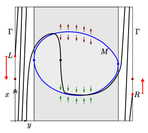
Figure 1: Canard solution of the system with convex slow curve: the base strip is shadowed

In backward time, the trajectory is quickly attracted to the repelling part of the slow curve, then moves slowly to the left until reaches the reverse jump point, jumps, and continues slow motion along the $y$-axis while rotating along the $x$-axis, up to the intersection with $\Gamma$. Denote the point of the intersection by $L(\varepsilon)$. This trajectory is canard, because it has a segment which is close to the repelling part of the slow curve.

As $\varepsilon>0$ decreases, “fast” parts of the trajectory become more vertical, and the number of rotations during the after-jump motion increases. Therefore, the point $R(\varepsilon)$ moves upwards, and $L(\varepsilon)$ moves downwards. By continuity, there exists $\varepsilon_{1}$ such that for $\varepsilon=\varepsilon_{1}$ these two points coincide: $R(\varepsilon_{1})=L(\varepsilon_{1})$. This gives us canard limit cycle. As $\varepsilon>0$ continues decreasing, new coincidense occurs for some $\varepsilon=\varepsilon_{2}$, $0<\varepsilon_{2}<\varepsilon_{1}$, and so on. Therefore, for the sequence of parameter values $\varepsilon=\varepsilon_{k}$, accumulating to $0$, the system has canard limit cycles. By choosing initial point close enough to the reverse jump point, it is possible to make these cycles stable. When we perturb initial point slightly, corresponding values of $\varepsilon_{k}$ also perturb slighly, giving us “canard intervals”, whose existence is stated in Theorem 1.1.

When we consider more general case of nonconvex $M$ and $N>1$, the description becomes more complicated, but the main arguments still work. Let us assume that any two fold points lie on different vertical circles, and the initial point $w$ does not lie above or below any fold point. In this case, the trajectory which starts in $w$, in forward (backward) time falls to attracting (repelling) segment of $M$, moves slowly to the right (left) until reaches the fold point, jumps and either leaves the base strip or falls to other attracting (repelling) segment of $M$, and the process repeats until the trajectory leaves the base strip (see Fig. 2).

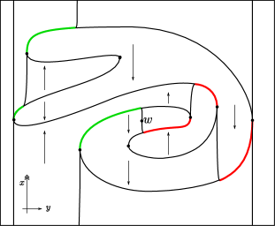
Figure 2: Nonconvex case: several jumps

The main difference with the convex case here is the possibility of several jumps. In fact, it does not affect heuristic arguments presented above, because they deal mostly with the after-jump rotations. However, to provide a rigorous proof of the main results and in particular to calculate the number of limit cycles, it does not suffice to use only the ideas discussed. Instead, we have to perform accurate analysis of the Poincaré map from $\Gamma$ to itself, which is discussed in the next sections.

3 Poincaré map

Note that the function $g$ is bounded away from zero, so we can divide the system (1) by $g$, thus re-scaling the time: this does not change the desired properties of its solutions (we are interested only in phase curves), and the system with the new function $f$ will satisfy the same nondegenericity assumtions. Thus without loss of generality we can assume $g=1$ in (1).

Consider Poincaré map $P_{\varepsilon}:\Gamma\to\Gamma$. The slow motion is constant (and bounded away from $0$), so $P_{\varepsilon}$ is a well-defined diffeomorphism of a circle. Its periodic (in particular, fixed) points correspond to closed solutions of the system. Denote the graph of $P_{\varepsilon}$ by $\gamma_{\varepsilon}$. Fixed points of the Poincaré map correspond to the intersection points of the graph with the diagonal $\mathcal{D}:=\{y=x\}$. Note, that in terms of the previous section, $P_{\varepsilon}(L(\varepsilon))=R(\varepsilon)$.

The derivative of the Poincaré map in any point $x_{0}\in\Gamma$ can be easily calculated by integrating the equation of variations. Namely, let $x=x(y;x_{0},\varepsilon)$ be the phase curve with the initial condition $x(-\pi;x_{0},\varepsilon)=x_{0}$. Then, $P_{\varepsilon}(x_{0})=x(\pi;x_{0},\varepsilon)$ and

$$P^{\prime}_{\varepsilon}(x_{0})=\left.\frac{\partial P_{\varepsilon}(x)}{\partial x}\right|_{x=x_{0}}=\frac{\partial x}{\partial x_{0}}(\pi;x_{0})=\exp\frac{1}{\varepsilon}\int_{-\pi}^{\pi}f^{\prime}_{x}(x(y;x_{0},\varepsilon),y,\varepsilon)\,dy.$$ (3)

Near the attracting (repelling) parts of the slow curve $M$, the function under the intergral sign is negative (positive), and the trajectories attract (repell) each other while moving in these areas. Corresponding parts of the trajectories contribute contraction (expansion) to the derivative of Poincaré map. In “most of the cases” $\int f^{\prime}_{x}(x,y,\varepsilon)dy\neq 0$ and either contraction or expansion dominates, thus giving either exponentially small or exponentially big derivative with respect to $\varepsilon$.

It turns out that it is possible to replace actual trajectory in the right-hand side of (3) with so-called singular trajectory (or contour), which is defined as follows. For every point $w\in B\setminus M$, which does not lie above or below any fold point of $M$, recall the description of the trajectory which pass through $w$ traced in backward and forward time up to exit from $B$ (see section 2). Assume that all phases of fast motion in this description are strictly vertical. Then we obtain a picewise-smooth curve in the base strip which consists of vertical segments and arcs of the slow curve M, interchanging each other. Call this curve singular trajectory (or contour) of $w$ and denote it by $Z(w)$. This curve is in a sense a limit (as $\varepsilon\to 0$) of the trajectories with the initial condition $w$. The part of the contour to the right of $w$ (which corresponds to the trajectory in forward time) is denoted by $Z^{-}(w)$, and the part to the left of $w$ (which corresponds to backward time) is denoted by $Z^{+}(w)$.

The following Lemma represents the fact that the derivative of the Poincaré map is controlled (with given precision) by the contour of the corresponding trajectory. It means that the main contribution to the derivative is made by the segments of slow motion near the arcs of the slow curve. This contribution dominates over the one of the jumps and the after-jump rotations.

Lemma 3.1.

Fix some $\delta>0$. Fix some vertical interval $J$, which intersects attracting part of $M$ and $\delta$-bounded from repelling part of $M$ (and therefore from fold points). Let $u$ be coordinate on $J$. Consider Poincaré map $Q:J\to\Gamma$ in forward time. Then for any $w\in J$,

$$\log\left.\frac{dQ(u)}{du}\right|_{J}=\frac{1}{\varepsilon}\left[\int_{Z^{-}(w)}f^{\prime}_{x}(x,y,0)\,dy+o(1)\right].$$ (4)

Obviously, $Z^{-}(w)$ does not depend on choice of $w\in J$. The remainder term $o(1)\to 0$ as $\varepsilon\to 0$ uniformly in choice of $J$ provided $\delta$ is fixed.

Lemma 3.2.

Let $w\in B\setminus M_{\delta}$, where $M_{\delta}$ is $\delta$-neighborhood of $M$, and $y(w)$ ($y$-coordinate of $w$) is $\delta$-far from $y(G)$ for any fold point $G$. Consider actual trajectory that pass through $w$, and denote its initial condition on $\Gamma$ by $x_{0}$. Then

$$\log P^{\prime}_{\varepsilon}(x_{0})=\frac{1}{\varepsilon}\left[\int_{Z(w)}f^{\prime}_{x}(x,y,0)\,dy+o(1)\right].$$ (5)

The proof of these Lemmas is given in [3] (see Lemma 5.4 and Lemma 7.3 there), and rely heavily on the analysis of the after-jump rotations from [2] (see Theorem 4.3 there, which is reformulated as Theorem 4.6 in [3]).

4 Shape of the graph of $P_{\varepsilon}$

Our goal is to describe the shape of $\gamma_{\varepsilon}$ and its dependence on $\varepsilon$. The following description goes back to Shape Lemma in [1], where it is proved for a particular example.

Fix some vertical interval $J^{+}$ (resp. $J^{-}$) in the phase space, which intersects repelling (attracting) part of the slow curve close enough to far left (far right) fold point and is bounded from attracting (repelling) part of the slow curve. (See Fig. 3.)

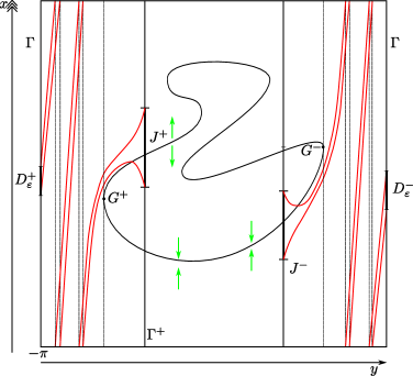
Figure 3: Phase curves near main jump points

Definition 4.1.

A trajectory is called a duck (canard) if and only if it intersects $J^{+}$.

Consider the projection of $J^{+}$ (resp., $J^{-}$) to $\Gamma$ along phase curves in backward (forward) time. Denote it by $D^{+}_{\varepsilon}$ (resp, $D^{-}_{\varepsilon}$). Note that all the trajectories that intersect $D^{+}_{\varepsilon}$ are ducks. Lemma 3.1 (applied to the system with the time reversed if necessary) implies immediately that $|D^{+}_{\varepsilon}|=O(\exp(-C_{1}/\varepsilon))$ and $|D^{-}_{\varepsilon}|=O(\exp(-C_{2}/\varepsilon))$ for some positive $C_{1},\ C_{2}$. The trajectory with the inital condition $x_{0}\in\Gamma\setminus D^{+}_{\varepsilon}$ does not intersect $J^{+}$. Therefore, it is attracted to the attracting part of the slow curve rather quickly (the speed is controlled by the distance between $J^{+}$ and the reverse jump point), and then moves near attracting parts of the slow curve only, accumulating contraction (see the integral (3)). It also have to intersect $J^{-}$ and therefore $D^{-}_{\varepsilon}$. Lemma 3.2 implies that in this case the derivative of the Poincaré map is exponentially small. On the other hand, appliyng the same arguments to the system with time reversed, we have that outside of $D^{-}_{\varepsilon}$, the inverse Poincaré map $P^{-1}_{\varepsilon}$ has exponentially small derivative. Informally speaking, it means that almost all the circle in the pre-image (except for very small interval) is mapped into very small interval in the image, while the exceptional interval in the pre-image is mapped into almost all the circle in the image.

Geometrically, this means that the graph $\gamma_{\varepsilon}$ belongs to the union $\Pi^{+}\cup\Pi^{-}$ of exponentially thin strips: vertical $\Pi^{+}=D^{+}_{\varepsilon}\times S^{1}$ and horizontal $\Pi^{-}=S^{1}\times D^{-}_{\varepsilon}$. Outside of the rectangle $K_{\varepsilon}=\Pi^{+}\cap\Pi^{-}$, the slope of $\gamma_{\varepsilon}$ is either exponentially big or exponentially small (see Fig. 4).

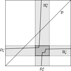
Figure 4: Graph of Poincaré map

Monotonicity arguments similar to the ones discussed in section 2 show that as $\varepsilon\searrow 0$, rectangle $K_{\varepsilon}$ moves from bottom-right to top-left corner, making infinitely many rotations. (See Monotinicity Lemmas in [1] and [2] for details.)

In this paper, we are interested only in limit cycles that correspond to fixed points of Poincaré map (i.e. making $1$ rotation along the $y$-axis). They are born (or die) when the diagonal $\mathcal{D}$ tangents the graph $\gamma_{\varepsilon}$. Such a tangency is possible only at the points where the slope of $\gamma_{\varepsilon}$ is equal to $1$. We will call such points neutral, applying this term both to the points on the graph $\gamma_{\varepsilon}$ and to the corresponding values of argument (i.e. roots of the equation $P^{\prime}_{\varepsilon}(x)=1$). Note that all neutral points belong to $K_{\varepsilon}$, and therefore the fixed points can be born only inside $K_{\varepsilon}$, thus giving us pairs of repelling and attracting canard cycles. (All points in $K_{\varepsilon}$ correspond to canard solutions because they lie over $D^{+}_{\varepsilon}$.)

For every neutral point $x$, consider second derivative $P^{\prime\prime}_{\varepsilon}(x)$, and call $x$ generating (resp., annihilating) if $P^{\prime\prime}_{\varepsilon}(x)<0$ (resp., $P^{\prime\prime}_{\varepsilon}(x)>0$). We may impose nondegenicity conditions, such that $P^{\prime\prime}_{\varepsilon}(x)\neq 0$ in every neutral point $x$. Consider a projection $\Delta(x,y)=x-y$ along the diagonal $\mathcal{D}$. It turns out (this will be discussed below) that for any given system for $\varepsilon$ small enough the number of neutral points is alwas the same (does not depend on $\varepsilon$; see section 5) and the order of their projections under $\Delta$ is fixed as well (see section 6). In this case, actual maximal number of canard cycles is defined by the order of births and deaths, which is controlled by the order of generating and annihilating neutral points under the projection map $\Delta$, and thus does not depends on $\varepsilon$. This gives us the number $k$ from Theorem 1.1. Rolle’s Theorem implies that $k\leq N$. Neutral points depend on $\varepsilon$ continiously, therefore on every turn of $K_{\varepsilon}$ there exists an open interval of $\varepsilon$’s, on which the maximal number (which is $2k$) of canard cycles are born. Such intervals accumulate to $0$, and their existence is the main result of theorem 1.1.

The rest of paper is devoted to the analysis of neutral points. We first prove that the number of neutral points is bounded by the number of folds of $M$ and show how it can be calculated explicitly (see section 5). Then we discuss the order of births and deaths of canard cycles (see section 6). Finally, we will contstruct an open set of systems with maximal number of limit cycles $k=N$ (section 7).

5 Neutral points

Consider a trajectory, that passes through some point $w\in\mathring{B}\setminus M$ (see the description in section 2). The part of the trajectory to the left from $w$ lies near the repelling arcs of the slow curve; the part to the right from $w$ lies near the attracting parts of the slow curve. We will say that at $w$ the trajectory passes through duck (or canard) jump: the transition from unstable part of the slow curve to the stable one. Let $S$ be an arc of the slow curve $M$ between two consequent fold points (maximal arc). It is well-known [6] that there exists invariant curve $S_{\varepsilon}$ that tends to $S$ as $\varepsilon\to 0$. This curve is called (maximal) true slow curve. It is not unique, but all such curves are exponentially close to each other and we can pick a suitable one.

For every maximal arc of $M$, consider corresponding maximal true slow curve (see Fig. 5).

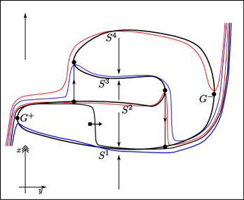
Figure 5: Maximal true slow curves and duck jump

Extend them in the backward time to $\Gamma$, and denote corresponding intersection points by $u_{1},\ldots,u_{2N}$ (enumeration is consequent, even numbers correspond to the repelling curves and odd to the attracting ones; obviously, they should interchange). Put by definition $u_{2N+i}\equiv u_{i}$. Enumerate corresponding slow curves as $S^{1},\ldots,S^{2N}$, and true slow curves as $S^{1}_{\varepsilon},\ldots,S^{2N}_{\varepsilon}$ respectively.

The trajectory, that passes through canard jump from $S_{2l}$ can fall after the jump either to $S_{2l-1}$ or to $S_{2l+1}$. Consider the first case. It becomes possible if the initial condition $u$ belongs to the interval $(u_{2l-1},u_{2l})$, i.e. lies below $u_{2l}$. When we move $u$ a bit upward (closer to $u_{2l}$), the whole trajectory moves closer to $S^{2l}_{\varepsilon}$. Thus the duck jump moves to the right. It means that the trajectory will spend more time near the repelling part of the slow curve and less time near the attracting part. Therefore, it will accumulate more expansion and less contraction, and the derivative of the Poincaré map increase monotonically on this interval.

Similar arguments show that the derivative of the Poincaré map decreases monotonically on interval $(u_{2l},u_{2l+1})$. It follows that the Poincaré map has picewise-monotonic derivative with exactly $N$ intervals of growth and $N$ intervals of decrease. Therefore, the equation $P^{\prime}(x)=1$ can have no more than $2N$ roots. This proves the estimate for the number of the neutral points, and therefore of the canard cycles.

Actual number of neutral points can be calculated as the number of zeroes of logarithmic derivative $\log P_{\varepsilon}^{\prime}(x)$. It follows from the analysis above that this derivative, presented as an integral (3), reaches its maximal and minimal values in the points that corresponds to the maximal true slow curves. Lemma 3.2 (with some modifications) implies that these values can be calculated as integrals over special contours, which contain maximal arcs of the slow curve. Thus the number of the neutral points equals to the number of sign changes of these values. It does not depend on $\varepsilon$ and can be effectively calculated.

6 Order of neutral points

Lift the rectangle $K_{\varepsilon}$ to the universal cover of the two-torus continuosly with respect to $\varepsilon$. Pick two arbitrary neutral points $\xi,\,\eta\in\gamma_{\varepsilon}$ from this lifted rectangle. Then we can define the difference between their projections $\Delta(\xi)-\Delta(\eta)$, assuming that $\Delta=x-y$, where $x$ and $y$ are coordinates on universal cover. (We need these precuations, because in general case the difference between two points on a circle is not defined.) In this section, we show that for any two neutral points the sign of this difference does not depend on $\varepsilon$.

The main idea is to show that the segment $[\xi,\eta]\subset K_{\varepsilon}$ is either “almost vertical” or “almost horizontal”. In the first case, if $\xi$ is top end of the segment and $\eta$ is bottom end, then $\Delta(\xi)-\Delta(\eta)>0$. In the second case, if $\xi$ is left end and $\eta$ is right end, then $\Delta(\xi)-\Delta(\eta)>0$, and so on.

Consider two trajectories which correspond to neutral points (call them neutral trajectories). Due to Lemma 3.2, they should lie near some contours with zero integrals (call such contours neutral as well). Note, that this implies that the measure of basins of limit cycles is bounded away from $0$: these cycles lie in different areas of the phase space, which are separated by neutral solutions which are close to fixed neutral contours.

Consider first forward-time parts of these contours (which are denoted by $Z^{+}$). They both contain the far right fold point and therefore have some nonempty intersection. Denote far left point of this intersection by $T$. To the left of $T$, the corresponding contours (and therefore actual trajectories) are bounded away from each other. To the right of $T$, the trajectories follow the same attracting arcs of the slow curve, and therefore attract each other.

Consider Poincaré map from some interval $J^{\prime}\ni T$ to $\Gamma$ in forward time. Then the rate of the attraction is given by Lemma 3.1 and is defined by the integral $f^{\prime}_{x}$ over intersection of the contours. This integral does not depend on $\varepsilon$ and can be calculated explicitly. The distance between these trajectories when they approach $\Gamma$ is the distance between the $y$-coordinates of corresponding neutral points. It follows immediately that $|y(\xi)-y(\eta)|=O^{*}(\exp(-C^{-}/\varepsilon))$ for some $C^{-}>0$.

Applying the same arguments to the system with time reversed, we obtain similar statement for $x$-coordintes: $|x(\xi)-x(\eta)|=O^{*}(\exp(-C^{+}/\varepsilon))$ for some $C^{+}>0$.

Consider the slope of the segment $[\xi,\eta]$, which is equal to

$$\frac{|y(\xi)-y(\eta)|}{|x(\xi)-x(\eta)|}=O^{*}\left(\exp\frac{C^{+}-C^{-}}{\varepsilon}\right).$$ (6)

Again, we may impose additional nondegenericity conditions and assume that $C^{+}\neq C^{-}$. This means that the slope is either exponentially big or exponentially small, what implies the necessary assertion immediately.

This proves that the order of neutral points under the projection $\Delta$ is fixed and thefore the maximal number of canard cycles $k$ is well-defined. It finishes the proof of Theorem 1.1.

7 Duck farm

The discussion above shows that we can translate “dynamical” questions (e.g. about limit cycles, Poincaré map and so on) into geometrical/combinatorial language which involves the shape of the slow curve $M$ and values of integrals of $f^{\prime}_{x}$ over some arcs of $M$. As an application of this approach, we pick an arbitrary $N>1$ and construct a system with maximal number of canard cycles: $k=N$. In fact, this example provides an open set of such systems, because all conditions imposed on the system during the construction of this example are open. To simplify the notation, we consider only the case $N=3$, but extension of these arguments to the general case is strightforward.

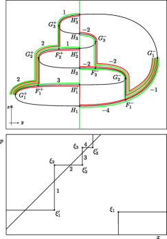
Figure 6: The system with maximal number of ducks

The key ingredient of the construction is the shape of the slow curve, see Fig. 6, top part. We demand here the depicted contours to be neutral, and the integrals of $f^{\prime}_{x}$ over the corresponding arcs to be equal to corresponding values (e.g. $\int_{H_{1}F_{1}^{-}}f^{\prime}(x,y,0)\,dy=-4$, and so on).

This system has $2N$ neutral contours, and therefore $2N$ neutral points on the graph $\gamma_{\varepsilon}$. It follows from the previous results, that for such a system, the graph looks like a “staircase”, where “lengths” and “heights” of the steps monotonically decrease (see Fig. 6, bottom part). This can be shown by an explicit calculation of the corresponding exponential rates that control “lengths” and “heights” of the steps (see the description in the previous section). They depend only on the integrals over the arcs which we control.

Due to the shape of the graph of Poincaré map, it follows that the order of the bifurcations of limit cycles is the following: first we have $N$ births and then we have $N$ deaths. During every birth a pair of cycles appear, therefore the number of canard cycles here is maximal and equal to $2N$. Thus we have constructed the desired example. This proves Theorem 1.2.

References

- [1] (MR1852932) J. Guckenheimer and Yu. S. Ilyashenko The Duck and the devil: canards on the staircase Moscow Math. J., 1:1 (2001), 27–47.
- [2] I. V. Schurov Ducks on the torus: existence and uniqueness. Journal of Dynamical and Control Systems, 16:2 (2010), 267–300, arXiv 0910.1888
- [3] I. V. Schurov Canard cycles in generic fast-slow systems on the torus. Transactions of the Moscow Mathematical Society, 2010, 175-207.
- [4] (MR0643399) E. Benoît, J. F. Callot, F. Diener, M. Diener Chasse au canard. Collect. Math., 31–32 (1981), 37–119.
- [5] (MR0750298) E. F. Mishchenko and N. Kh. Rozov “Differential equations with small parameters and relaxation oscillations.” Plenum Press, 1980.
- [6] (MR0524817) N. Fenichel Geometric singular perturbation theory for ordinary differential equations. J. of Diff. Eq., 31 (1979), 53–98.