Random walk approach to spin dynamics in a two-dimensional electron gas with spin-orbit coupling

Abstract

We introduce and solve a semi-classical random walk (RW) model that describes the dynamics of spin polarization waves in zinc-blende semiconductor quantum wells. We derive the dispersion relations for these waves, including the Rashba, linear and cubic Dresselhaus spin-orbit interactions, as well as the effects of an electric field applied parallel to the spin polarization wave vector. In agreement with calculations based on quantum kinetic theory [P. Kleinert and V. V. Bryksin, Phys. Rev. B 76, 205326 (2007)], the RW approach predicts that spin waves acquire a phase velocity in the presence of the field that crosses zero at a nonzero wave vector, $q_{0}$. In addition, we show that the spin-wave decay rate is independent of field at $q_{0}$ but increases as $(q-q_{0})^{2}$ for $q\neq q_{0}$. These predictions can be tested experimentally by suitable transient spin grating experiments.

I Introduction

Spin-orbit (SO) coupled two-dimensional electron systems are of great interest, both as model systems and as the active component of devices that control electron spin with electric fields.Dietl Unfortunately, the potential of the SO interaction to control electron spin comes with a price - the SO terms in the Hamiltonian break SU(2) spin symmetry. The violation of SU(2) means that electron spin polarization is not conserved, decaying instead with a characteristic spin memory time $\tau_{s}$. The mechanism by which SO coupling leads to spin memory loss has been intensively investigated in two-dimensional electron gases (2DEGs) in semiconductor quantum wells (QWs), as described in recent reviews.Fabian ; Wu In GaAs QWs and related systems, breaking of inversion symmetry allows SO coupling that is linear in the electron wave vector $\boldsymbol{k}$.Rashba1 ; Rashba2 ; Rashba3 The SO terms in the Hamiltonian can be viewed as effective magnetic fields that act only on the electron spin, with magnitude and direction that vary with $\boldsymbol{k}$. The loss of spin memory in the effective magnetic field, $\boldsymbol{b}(\boldsymbol{k})$, takes place through the D’yakonov-Perel’ (DP) mechanism.DP1 ; DP2 ; DP3 ; DP4 In this process the electron spin precesses during its ballistic motion between collisions; each time it is scattered $\boldsymbol{b}(\boldsymbol{k})$ and consequently the precession vector, $\boldsymbol{\Omega}(\boldsymbol{k})$, change. The net result is exponential decay of spin polarization at a rate approximately equal to $\Omega^{2}\tau$, where $\tau$ is the mean time between collisions.

There exist two distinct contributions to $\boldsymbol{b}(\boldsymbol{k})$, the Rashba termRashba2 ; Rashba3 arising from asymmetry of the confining potential and the Dresselhaus termDresselhaus originating in the intrinsic inversion asymmetry of the GaAs crystal structure. A prescription for lengthening spin lifetime in QWs of III-V semiconductors by tuning the Rashba coupling strength ($\alpha$) to equal the linear Dresselhaus coupling ($\beta_{1}$) was proposed by Schliemann et al.SL Recently it was recognized that this mechanism amounts to a restoration of SU(2) symmetry even in the presence of anisotropic SO interactions.SU2 The main purpose of this paper is to assess theoretically to what extent tuning SO interactions can be expected to increase the distance over which electron spin polarization can propagate without decay.

The potential to extend the spin propagation length despite DP spin memory decay is based on the strong correlation between the electron’s displacement in space and the rotation of its spin on the Bloch sphere. An important step toward a quantitative theory of such correlations was made by Burkov et al.MD and Mishchenko et al.,Mish who derived equations of motion that describe the coupling of spin and charge current degrees of freedom in (001) GaAs QWs. Initially only the linear Rashba SO coupling was examined, subsequently Bernevig et al.SU2 and Stanescu and Galitski cubic extended the theory to include the linear and cubic Dresselhaus terms, respectively.

The equations of motion can be solved to obtain the normal modes of the coupled system, which are waves of mixed electrical current and spin polarization. There exist four such modes, reflecting three spin degrees of freedom ($S_{x},S_{y}$, and $S_{z}$) and the charge density, $n$. For wave vectors, $\boldsymbol{q}$, parallel to the directions $[110]$ and $[1\bar{1}0]$, the four modes decouple into two pairs; in one the spin precesses in a plane containing $\boldsymbol{q}$ and the normal direction $\boldsymbol{\hat{z}}$, in the other the current is coupled to the component of in-plane spin polarization perpendicular to $\boldsymbol{q}$.

The spin precession mode is the one relevant to spin polarization memory. For example, the decay rate of this mode at $\boldsymbol{q}=0$ is precisely the DP decay rate, $1/\tau_{s}$. In the absence of spin-space correlation, the decay rate, $\gamma_{q}$, of a spin polarization wave would increase monotonically with $q$, i.e., $\gamma_{q}=1/\tau_{s}+D_{s}q^{2}$, where $D_{s}$ is the spin diffusion coefficient. Instead, it was predicted MD that for Rashba SO coupling the minimum decay rate occurs at nonzero wave vector, at which point $\gamma_{q}$ is approximately half the DP rate. Bernevig et al.SU2 showed theoretically that the minimum $\gamma_{q}$ is further reduced when both Rashba and linear Dresselhaus interactions are nonzero and vanishes when the strength of the two couplings is equal. The resulting “persistent spin helix” (PSH) was shown to be a conserved quantity of a newly found SU(2) symmetry that arises when $\alpha=\beta_{1}$ and the cubic Dresselhaus term ($\beta_{3}$) is zero.SU2 However, Stanescu and Galitski cubic showed that perfect SU(2) is broken when $\beta_{3}\neq 0$, leading to large, but not infinite, PSH lifetime. Recently, using the transient spin grating technique, Koralek et al.jake observed the PSH mode experimentally by independently tuning the Rashba and linear Dresselhaus couplings.

The question that arises is whether the PSH effect can be exploited to lengthen the distance that a packet of spin polarization can propagate in an applied electric field. In this paper we address this question by analyzing the effects of an in-plane electric ($E$) field on the spin-precession modes. We focus on $\boldsymbol{E}\parallel\boldsymbol{q}$, which is the orientation relevant to the drift of spin polarization. To predict the spin memory length it is necessary to determine how the applied field modifies both the real ($\Re$) and imaginary ($\Im$) parts of the normal-mode frequency, $\omega(q)$ of spin-polarization modes. The real part is related to the drift velocity whereas the imaginary part is related to the lifetime. The modification of $\Re\{\omega(q)\}$ is linear in $E$ (to lowest order), whereas the affect of $E$ on $\Im\{\omega(q)\}$ is quadratic. Kleinert and Bryksin KB ; KB2 recently have treated this to problem to linear order in $E$, using quantum kinetic theory, and obtained results for $\Re\{\omega(q)\}$.

In this work, we derive and solve equations of motion to quadratic order in $E$ using a random walk (RW) approach that is different from previous treatments of this problem. The advantages of our approach are physical transparency and mathematical simplicity. We construct a semiclassical random walk model that tracks the electron’s motion in real space and the propagation of its spin on the Bloch sphere. In Sec. II, we introduce the random walk model, derive the equations of motion in the absence of an $E$ field, and solve for the spin-wave dispersion relations. We compare the results thus obtained with the earlier quantum kinetic theory approaches.SU2 ; cubic In Sec. III, we include an in-plane $E$ field, obtaining the equations of motion and the dispersion relations to quadratic order. We use the dispersion relations to analyze the motion of a spin-polarization packet in the presence of the in-plane field, for different regimes of field strength. We illustrate the results by focusing on representative SO couplings: linear Dresselhaus coupling only, the SU(2) case where Rashba and Dresselhaus terms are equal, and the case of SU(2) broken by a small cubic Dresselhaus term. A brief summary is given in Sec. IV.

II Random walk model

As mentioned above, as an electron propagates between scattering events, SO coupling causes its spin to precess. Thus, as the electron performs an RW in real space, its spin performs an RW on the Bloch sphere. We consider a 2D electron gas with both structure and bulk inversion asymmetry. The SO Hamiltonian for conduction band electrons in a III-V semiconductor QW grown in the [001] direction (taken as $\boldsymbol{\hat{z}}$-direction) is given by,

$$H_{SO}=\boldsymbol{\Omega}\cdot\boldsymbol{s},$$ (1)

where,

$$\boldsymbol{\Omega}=2k_{F}\left\{\boldsymbol{\hat{x}}\left[\alpha-\beta_{1}-\frac{2\beta_{3}(v_{x}^{2}-v_{y}^{2})}{v_{F}^{2}}\right]v_{y}-\boldsymbol{\hat{y}}\left[\alpha+\beta_{1}-\frac{2\beta_{3}(v_{x}^{2}-v_{y}^{2})}{v_{F}^{2}}\right]v_{x}\right\},$$ (2)

$\boldsymbol{s}=\hbar\boldsymbol{\sigma}/2$ is the electron spin, $v_{x}$ and $v_{y}$ are the components of velocity in the [110] and [1$\bar{1}$0] directions, $\alpha$, $\beta_{1}$, and $\beta_{3}$ are dimensionless quantities describing the strength of the Rashba, linear, and cubic Dresselhaus spin-orbit couplings, respectively, and $k_{F}$ is the Fermi wave vector. Spins precess about the effective SO field according to

$$\frac{d\boldsymbol{s}}{dt}=\boldsymbol{\Omega}\times\boldsymbol{s}.$$ (3)

We assume that the impurity potential is short range so that there is no correlation between the scattering events. In the absence of the $E$ field, electrons perform an isotropic 2D random walk with $\boldsymbol{v}_{n}$ (velocity between the $n$th and $(n+1)$th scattering events) given by $v_{F}\boldsymbol{\hat{t}}_{n}$, where $\boldsymbol{\hat{t}}_{n}=(\cos\theta,\sin\theta)$ is a random two-dimensional unit vector with a uniform probability density $p_{n}(\theta)=1/2\pi$. The displacement from $n$th to $(n+1)$th step is given by

$$\boldsymbol{r}_{n+1}-\boldsymbol{r}_{n}=\boldsymbol{v}_{n}\tau,$$ (4)

where $\tau$ is the electron scattering time. In the following we consider $\Omega\tau$, the change in angle of the electron’s spin between scattering events, as a small parameter. In this case we can obtain from Eq. (3) the change in the spin direction during the mean-free time as a series expansion in $\Omega\tau$,

$$\Delta\boldsymbol{s}_{n}\equiv\boldsymbol{s}_{n+1}-\boldsymbol{s}_{n}=\boldsymbol{\Omega}_{n}\tau\times\boldsymbol{s}_{n}+\frac{1}{2}\boldsymbol{\Omega}_{n}\tau\times(\boldsymbol{\Omega}_{n}\tau\times\boldsymbol{s}_{n}),$$ (5)

where we retain terms to second order.

Let $P_{n}(\boldsymbol{r})$ be the probability that after $n$ steps of random walk the electron arrives at position $\boldsymbol{r}$ and $D_{n}(\boldsymbol{r};\boldsymbol{s})$ be the conditional probability that given the electron is at $\boldsymbol{r}$, its spin is $\boldsymbol{s}$. The joint probability $P_{n}(\boldsymbol{r})D_{n}(\boldsymbol{r};\boldsymbol{s})$ satisfies the following recursion relation:

$$P_{n+1}(\boldsymbol{r})D_{n+1}(\boldsymbol{r};\boldsymbol{s})=\langle P_{n}(\boldsymbol{r}-\boldsymbol{v}_{n}\tau)D_{n}(\boldsymbol{r}-\boldsymbol{v}_{n}\tau;\boldsymbol{s}-\Delta\boldsymbol{s}_{n})\rangle,$$ (6)

where $\langle\rangle$ denotes average over $\boldsymbol{\hat{t}}_{n}$, i.e., $\langle A_{n}\rangle=\int_{0}^{2\pi}A_{n}(\theta)p_{n}(\theta)d\theta$. Once $P_{n}(\boldsymbol{r})D_{n}(\boldsymbol{r};\boldsymbol{s})$ is determined, the magnetization can be obtained from the following integral on the Bloch sphere:

$$\boldsymbol{m}_{n}(\boldsymbol{r})=\int_{S^{2}}\boldsymbol{s}P_{n}(\boldsymbol{r})D_{n}(\boldsymbol{r};\boldsymbol{s})d\Sigma.$$ (7)

By substituting Eq. (6) into Eq. (7), we obtain,

$$\boldsymbol{m}_{n+1}(\boldsymbol{r})=\langle\int_{S^{2}}\boldsymbol{s}P_{n}(\boldsymbol{r}-\boldsymbol{v}_{n}\tau)D_{n}(\boldsymbol{r}-\boldsymbol{v}_{n}\tau;\boldsymbol{s}-\Delta\boldsymbol{s}_{n})d\Sigma\rangle.$$ (8)

Taylor series expansion on the right hand side of Eq. (8) yields,

$$\begin{split}\boldsymbol{m}_{n+1}(\boldsymbol{r})=&\langle\int_{S^{2}}[\boldsymbol{s}+\boldsymbol{\Omega}_{n}\tau\times\boldsymbol{s}+\frac{1}{2}\boldsymbol{\Omega}_{n}\tau\times(\boldsymbol{\Omega}_{n}\tau\times\boldsymbol{s})]\{P_{n}(\boldsymbol{r})D_{n}(\boldsymbol{r};\boldsymbol{s})\\ &-\boldsymbol{v}_{n}\tau\cdot\nabla[P_{n}(\boldsymbol{r})D_{n}(\boldsymbol{r};\boldsymbol{s})]+\frac{1}{2}\boldsymbol{v}_{n}\tau\cdot\nabla\nabla[P_{n}(\boldsymbol{r})D_{n}(\boldsymbol{r};\boldsymbol{s})]\cdot\boldsymbol{v}_{n}\tau\}d\Sigma\rangle.\end{split}$$ (9)

Again retaining terms to second order, we can write,

$$\boldsymbol{m}_{n+1}=\boldsymbol{I}_{1}+\boldsymbol{I}_{2}+\boldsymbol{I}_{3},$$ (10)

where,

$$\begin{split}\boldsymbol{I}_{1}=&\langle\int_{S^{2}}\boldsymbol{s}\{P_{n}(\boldsymbol{r})D_{n}(\boldsymbol{r};\boldsymbol{s})-\boldsymbol{v}_{n}\tau\cdot\nabla[P_{n}(\boldsymbol{r})D_{n}(\boldsymbol{r};\boldsymbol{s})]\\ &+\frac{1}{2}\boldsymbol{v}_{n}\tau\cdot\nabla\nabla[P_{n}(\boldsymbol{r})D_{n}(\boldsymbol{r};\boldsymbol{s})]\cdot\boldsymbol{v}_{n}\tau\}d\Sigma\rangle,\end{split}$$ (11)

$$\boldsymbol{I}_{2}=\langle\int_{S^{2}}[\boldsymbol{\Omega}_{n}\tau\times\boldsymbol{s}]\{P_{n}(\boldsymbol{r})D_{n}(\boldsymbol{r};\boldsymbol{s})-\boldsymbol{v}_{n}\tau\cdot\nabla[P_{n}(\boldsymbol{r})D_{n}(\boldsymbol{r};\boldsymbol{s})]\}d\Sigma\rangle,$$ (12)

and

$$\boldsymbol{I}_{3}(\boldsymbol{r})=\langle\int_{S^{2}}[\frac{1}{2}\boldsymbol{\Omega}_{n}\tau\times(\boldsymbol{\Omega}_{n}\tau\times\boldsymbol{s})]\{P_{n}(\boldsymbol{r})D_{n}(\boldsymbol{r};\boldsymbol{s})\}d\Sigma\rangle.$$ (13)

Upon performing the average over $\boldsymbol{\hat{t}}_{n}$, all terms that linear in $\boldsymbol{v}_{n}$ or $\boldsymbol{\Omega}_{n}$ vanish by symmetry, leading to,

$$\boldsymbol{I}_{1}=\boldsymbol{m}_{n}+\Pi_{op}\tau^{2}\boldsymbol{m}_{n},$$ (14)

$$\begin{split}\boldsymbol{I}_{2}=&-\boldsymbol{\hat{x}}\langle\Omega_{ny}v_{nx}\rangle\tau^{2}\frac{\partial m_{nz}}{\partial x}+\boldsymbol{\hat{y}}\langle\Omega_{nx}v_{ny}\rangle\tau^{2}\frac{\partial m_{nz}}{\partial y}\\ &+\boldsymbol{\hat{z}}\left(\langle\Omega_{ny}v_{nx}\rangle\frac{\partial m_{nx}}{\partial x}-\langle\Omega_{nx}v_{ny}\rangle\frac{\partial m_{ny}}{\partial y}\right)\tau^{2},\end{split}$$ (15)

$$\boldsymbol{I}_{3}=-\frac{\tau^{2}}{2}\left(\boldsymbol{\hat{x}}\langle\Omega_{yn}^{2}\rangle m_{nx}+\boldsymbol{\hat{y}}\langle\Omega_{xn}^{2}\rangle m_{ny}+\boldsymbol{\hat{z}}\langle\Omega_{n}^{2}\rangle m_{nz}\right),$$ (16)

where

$$\Pi_{op}\equiv\frac{1}{2}\left(\langle v_{x}^{2}\rangle\frac{\partial^{2}}{\partial x^{2}}+\langle v_{y}^{2}\rangle\frac{\partial^{2}}{\partial y^{2}}\right).$$ (17)

Taking the continuum limit $\boldsymbol{m}_{n}\rightarrow\boldsymbol{m}(t)$, $\left(\boldsymbol{m}_{n+1}-\boldsymbol{m}_{n}\right)/\tau\rightarrow d\boldsymbol{m}/dt$, and substituting into Eq. (10), we obtain the equation of motion for the magnetization vector. Resolving the vector equation into components yields three scalar equations,

$$\frac{1}{\tau}\frac{\partial m_{x}}{\partial t}=\Pi_{op}m_{x}-\frac{1}{2}\langle\Omega_{y}^{2}\rangle m_{x}-\langle\Omega_{y}v_{x}\rangle\frac{\partial m_{z}}{\partial x},$$ (18)

$$\frac{1}{\tau}\frac{\partial m_{y}}{\partial t}=\Pi_{op}m_{y}-\frac{1}{2}\langle\Omega_{x}^{2}\rangle m_{y}+\langle\Omega_{x}v_{y}\rangle\frac{\partial m_{z}}{\partial y},$$ (19)

$$\frac{1}{\tau}\frac{\partial m_{z}}{\partial t}=\Pi_{op}m_{z}-\frac{1}{2}\langle\Omega^{2}\rangle m_{z}+\langle\Omega_{y}v_{x}\rangle\frac{\partial m_{x}}{\partial x}-\langle\Omega_{x}v_{y}\rangle\frac{\partial m_{y}}{\partial y}.$$ (20)

Solving the equations of motion for eigenmodes with wave vector parallel to $\boldsymbol{\hat{x}}$ yields the dispersion relation,

$$\frac{i\omega_{\pm}(q)}{\tau}=\frac{1}{4}\left(2\langle\Omega^{2}\rangle-\langle\Omega_{x}^{2}\rangle\right)+\frac{1}{2}\langle v_{x}^{2}\rangle q^{2}\pm\sqrt{\frac{\langle\Omega_{x}^{2}\rangle^{2}}{16}+q^{2}\langle\Omega_{y}v_{x}\rangle^{2}}.$$ (21)

This dispersion relation corresponds to modes in which the spin polarization spirals in the $x$-$z$ plane. Note that $\omega(q)$ is purely imaginary so that for all wave vectors the spin-polarization wave decays exponentially with time. However, the dispersion relation differs from ordinary diffusion, where $i\omega\propto 1/\tau+Dq^{2}$. The difference can be traced to the terms in Eq. (15) that are proportional to the first derivative of spin density with respect to position - these terms are absent in the usual diffusion equation. The coefficients of these additional terms are the cross-correlation functions, $\left\langle\Omega_{x}v_{y}\right\rangle$ and $\left\langle\Omega_{y}v_{x}\right\rangle$, which shows explicitly that the anomalous diffusion is a consequence of the correlation between the electron’s motion in real space and the propagation of its spin on the Bloch sphere.

In the SU(2) case ($\alpha=\beta_{1}$ and $\beta_{3}=0$), Eq. (21) simplifies to,

$$i\omega_{\pm}(q)=\frac{1}{4}v_{F}^{2}\tau\left(q\pm q_{0}\right)^{2}\equiv D(q\pm q_{0})^{2},$$ (22)

where $D\equiv v_{F}^{2}\tau/4$ and $q_{0}\equiv 4k_{F}\beta_{1}$. The vanishing decay rate of the $\omega_{-}$ mode at $q=q_{0}$ indicates the appearance of a conserved quantity - a helical spin-polarization wave or “persistent spin helix”.SU2

The dispersion relations obtained above for the spiral polarization waves are the same as those obtained previously, including the cubic Dresselhaus term.SU2 ; cubic We note, however, that while the RW approach accurately describes the spiral coupling of $x$-$z$ components of spin, it does not capture the coupling between charge current and the $y$ component of spin that appears in the quantum kinetic formulation. This is because the RW approach does not include relaxation to the equilibrium state. In other words, between consecutive scattering events the electron’s spin precesses about $\boldsymbol{b}(\boldsymbol{k})$ but has no tendency to spiral in toward it. Thus the well-known current-induced spin polarization (CISP) effect Mish is not predicted. To recover CISP requires adding to Eq. (3) a phenomenological Gilbert damping term,

$$\frac{d\boldsymbol{s}}{dt}=\lambda_{G}\boldsymbol{s}\times\left(\boldsymbol{\Omega}\times\boldsymbol{s}\right),$$ (23)

where $\lambda_{G}$ is the damping parameter.

III Spin Helix dynamics in the presence of an electric field

In this section, we explore how the spin dynamics change in the presence of an $E$ field parallel to the wave vector of the spin spiral. To include the effect of $E$ we add a drift term to the velocity at each random walk step,

$$\boldsymbol{v}_{n}=v_{F}\boldsymbol{\hat{t}}_{n}+v_{d}\boldsymbol{\hat{x}},$$ (24)

where $v_{d}$ is the drift velocity assumed to be a linear function of $E$. We assume further that the electric field does not change the shape of the impurity potential and therefore the scattering probability density is still uniform.

The drift velocity modifies the precession vector, adding a fixed precession

$$\boldsymbol{\Omega}_{d}\equiv-2\boldsymbol{\hat{y}}k_{F}\left[\alpha+\beta_{1}-\frac{2\beta_{3}(v_{x}^{2}-v_{y}^{2})}{v_{F}^{2}}\right]v_{d},$$ (25)

to $\boldsymbol{\Omega}_{n}$ at each step of the random walk. Substituting and following the same strategy as before, we obtain,

$$\boldsymbol{I}_{1}(\boldsymbol{E})=\boldsymbol{I}_{1}-v_{d}\tau\frac{\partial\boldsymbol{m}}{\partial x},$$ (26)

$$\boldsymbol{I}_{2}(\boldsymbol{E})=\boldsymbol{I}_{2}+\boldsymbol{\Omega}_{d}\tau\times\boldsymbol{m},$$ (27)

$$\boldsymbol{I}_{3}(\boldsymbol{E})=\boldsymbol{I}_{3},$$ (28)

where the $\boldsymbol{I}_{1,2,3}(\boldsymbol{E})$ are the quantities $\boldsymbol{I}_{1,2,3}$ evaluated in the presence of the electric field. The field alters the equations of motion in two ways. First, new terms appear that are linear in $E$. The new term added to $\boldsymbol{I}_{1}$ converts the time derivative of $\boldsymbol{m}$ to the convective derivative, that is the time derivative in a frame moving with the drifting electrons. The term added to $\boldsymbol{I}_{2}$ indicates that the $E$ field introduces uniform precession about the $\boldsymbol{\hat{y}}$ axis, when viewed in the frame co-moving with $\boldsymbol{v}_{d}$. The second type of modification is quadratic in $E$; the field increases $\langle\Omega_{y}^{2}\rangle$ by the additive factor $\Omega_{d}^{2}$ and the mean-square velocity $\langle v_{x}^{2}\rangle$ by the factor $\langle v_{d}^{2}\rangle$.

Solving for normal modes with wave vector parallel to $\boldsymbol{\hat{x}}$, we obtain

$$i\omega_{\pm}(q)=\frac{1}{4}\left(2\langle\Omega^{2}\rangle-\langle\Omega_{x}^{2}\rangle\right)\tau+\frac{1}{2}\langle v_{x}^{2}\rangle\tau q^{2}+iv_{d}q\pm\sqrt{\frac{\langle\Omega_{x}^{2}\rangle^{2}\tau^{2}}{16}+\left(q\langle\Omega_{y}v_{x}\rangle\tau+i\Omega_{d}\right)^{2}}.$$ (29)

To linear order in $E$, this dispersion relation is the same as that obtained by Kleinert and Bryksin.KB ; KB2 In the presence of the electric field $\omega(q)$ acquires a real part, which describes the propagation of spin polarization. Equation (29) also describes the modifications of the spin polarization lifetime that appear at second order in $E$. In the following we discuss the spin dynamics that emerge from this dispersion relation for representative SO Hamiltonians.

III.1 SU(2) case

For the case of $\alpha=\beta_{1},\beta_{3}=0$, the dispersion relation simplifies to,

$$i\omega_{\pm}(q)=D\left(1+2\lambda^{2}\right)\left(q\pm q_{0}\right)^{2}+iv_{d}\left(q\pm q_{0}\right),$$ (30)

where $\lambda\equiv v_{d}/v_{F}$. To distinguish the lifetime and propagation effects we write the dispersion relation in the form,

$$i\omega(q)=\gamma(q)+i\dot{\phi}(q),$$ (31)

where $\gamma(q)$ is the decay rate and $\dot{\phi}(q)$ is the rate of phase advance. The real and imaginary parts of $i\omega_{-}(q)$, corresponding to the longer lived of the two modes, are plotted in Fig. 1. As is apparent from Fig. 1, the spin polarization lifetime, $1/\gamma_{-}(q)$ remains infinite at the PSH wave vector, despite the presence of the electric field. This result is consistent with the theoretical prediction that at the SU(2) point the spin helix generation operators commute with all perturbation terms that are not explicitly spin dependent.SU2 However, the field increases the effective diffusion constant by the factor $\lambda^{2}$ so that the decay rate for $q\neq q_{0}$ increases rapidly when the drift velocity approaches the thermal velocity of the electrons. The spin helix generation operators won’t commute with the Hamiltonion if there exists a spatial disorder of SO interactions.Sherman1 ; Sherman2

The rate of phase advance [plotted in Fig. 1] vanishes at $q=q_{0}$, i.e., the PSH is stationary, despite the fact that the Fermi sea of electrons is moving by with average velocity $\boldsymbol{v}_{d}$. Moreover, spin spirals with $q<q_{0}$ will appear to move backward, that is, opposite to the direction of electron flow. Although unusual, this property can be understood by considering the spin dynamics in a frame moving with velocity $\boldsymbol{v}_{d}$. In this frame $\boldsymbol{E}$ parallel to $\boldsymbol{\hat{x}}$ is perceived as a precession vector $\boldsymbol{\Omega}_{d}=-4\beta_{1}v_{d}\boldsymbol{\hat{y}}=-v_{d}q_{0}\boldsymbol{\hat{y}}$. Therefore in the moving frame $\phi_{\pm}(x^{\prime},t^{\prime})=\pm qx^{\prime}-v_{d}q_{0}t$. Transforming back to the laboratory frame then yields $\dot{\phi}_{\pm}(q)=v_{d}(q\pm q_{0})$.

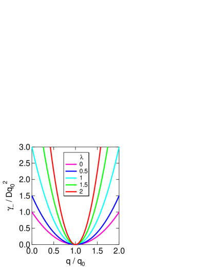
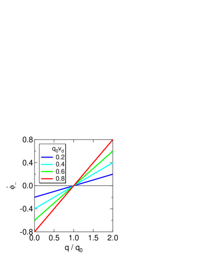
Figure 1: (Color online) The dispersion relations for (a) the decay rate and (b) the rate of phase change of the SO enhanced mode in the SU(2) case. (a) The decay rate $\gamma_{-}(q)$ increases with the drift velocity ($\lambda\equiv v_{d}/v_{F}$) but always vanishes at the resonant wave vector $q_{0}$. (b) The rate of phase change $\dot{\phi}_{-}(q)$ is proportional to the drift velocity $v_{d}$ and it crosses zero at the resonant wave vector $q_{0}$.

The nature of spin propagation at the SU(2) symmetry point can be made more clear if we Fourier transform from the wave vector to spatial domain. If we inject a $\delta$-function stripe of $z$ polarized spins at $x=0$, the space-time evolution of $S_{z}$ is proportional to the propagator, $G_{z}(x,t)$, where

$$G_{z}(x,t)\propto\int dqe^{iqx}\left(A_{+}e^{-i\omega_{+}t}+A_{-}e^{-i\omega_{-}t}\right),$$ (32)

where $A_{+}$ and $A_{-}$ are the weighting factors for the passive and active modes, respectively and $A_{+}=A_{-}=1/2$ in the SU(2) case. Upon substituting the dispersion relations $\omega_{\pm}(q)$, we obtain,

$$G_{z}(x,t)\propto\frac{1}{\sqrt{Dt}}\cos(q_{0}x)\exp{\left[-\frac{(x-v_{d}t)^{2}}{4Dt}\right]}.$$ (33)

The spin propagator is the product of a Gaussian envelope function and a static spin wave with wave vector $q_{0}$. The envelope function is the one-dimensional diffusion propagator with width proportional to $\sqrt{Dt}$ and drift velocity $v_{d}$. An illustration of the space-time evolution described by this propagator is provided Fig. 2, for a drift velocity $v_{d}=2Dq_{0}$. Note that the phase of the spin wave modulated by the Gaussian envelope remains stationary as the packet drifts and diffuses. This contrasts with the more familiar wave packet, where the modulated wave and envelope functions both propagate, albeit with velocities that may differ.

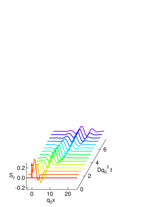
Figure 2: (Color online) The space-time evolution of $S_{z}$ with a normalized $\delta$-function injection at $x=0,t=0$, and drift velocity $v_{d}=2Dq_{0}$ in the SU(2) case. The spin polarization develops into a conserved stationary wave with a Gaussian wave packet.

III.2 SU(2) broken by cubic Dresselhaus term

When SU(2) is exact, the integral of the Gaussian envelope function is conserved, even in the presence of an $E$ field. However, Stanescu and Galitski cubic have shown theoretically that $\beta_{3}$, which is nonzero in real systems, breaks SU(2). Koralek et al. jake verified experimentally that $\beta_{3}$ is indeed the factor that limits PSH lifetime in experiments on (001) GaAs quantum wells. In this section we calculate the dispersion relation and spin packet time evolution in the presence of a small cubic Dresselhaus term.

It was shown previously that when $\beta_{3}$ is small, the maximum lifetime occurs when the Rashba interaction $\alpha=\beta_{1}-\beta_{3}$ (Ref. cubic, ). We consider a QW with Rashba coupling tuned to this value and assume that $\beta_{3}\ll\beta_{1}$. This condition is met in QWs in the 2D limit, where $k_{F}d\ll 1$ ($d$ is the well width). In this case the dispersion relation in the presence of the electric field can be written as

$$i\omega_{\pm}(q)\cong 6Dk_{F}^{2}\beta_{3}^{2}+D\left(q\pm q_{0}\right)^{2}+iv_{d}\left(q\pm q_{0}\right)\mp iv_{d}\Delta q,$$ (34)

where $q_{0}\equiv 4k_{F}(\beta_{1}-\beta_{3})$ and $\Delta q=2k_{F}\beta_{3}$. Performing the Fourier transform to obtain the space-time evolution of a spin packet, we obtain,

$$G_{z}(x,t)\propto\frac{1}{\sqrt{Dt}}e^{-6Dk_{F}^{2}\beta_{3}^{2}t}\cos(q_{0}x-v_{d}\Delta qt)\exp{\left[-\frac{(x-v_{d}t)^{2}}{4Dt}\right]}.$$ (35)

In the presence of the cubic Dresselhaus interaction the integral of the Gaussian envelope is no longer conserved. The decay rate can be written in the form,

$$\gamma=\frac{3}{8}Dq_{0}^{2}\left(\frac{\beta_{3}}{\beta_{1}}\right)^{2},$$ (36)

illustrating that although the decay rate is nonzero, it is reduced relative to the DP relaxation rate by a factor $\approx(\beta_{3}/\beta_{1})^{2}$. This ratio is expected theoretically,Winkler and has been verified experimentally,jake to be determined by the relation,

$$\frac{\beta_{3}}{\beta_{1}}=\frac{k_{F}^{2}d^{2}}{4\pi^{2}}.$$ (37)

For quite reasonable QW parameters a $\beta_{3}$ to $\beta_{1}$ ratio of 1:100 can be achieved, equivalent to a lifetime enhancement relative to the DP spin memory time on the order of $10^{4}$.

III.3 Linear Dresselhaus coupling

Finally, we consider a fully symmetric well in which only the linear Dresselhaus coupling exists. To make comparison with the SU(2) situation, we set the strength of the linear Dresselhaus coupling be $2\beta_{1}$, so that the resonant wave vector is at $q\simeq q_{0}=4k_{F}\beta_{1}$. The dispersion relations $\gamma_{-}(q)$ and $\dot{\phi}_{-}(q)$ obtained by substituting $\alpha=\beta_{3}=0$ and replacing $\beta_{1}$ by $2\beta_{1}$ in Eq. (29) are plotted in Fig. 3. Some qualitative features of the dispersion relations are similar to the SU(2) case, in that $\gamma_{-}(q)$ has a global minimum and $\dot{\phi}_{-}(q)$ crosses zero at $q\simeq q_{0}$. The most important difference is that the minimum $\gamma_{-}(q)$ does not reach zero, and therefore the spin spiral does decay. In the limit of low electric field, the lifetime of the spin spiral is only about a factor of 2 longer than the $q=0$ (DP) lifetime.

The propagation of a spin packet in the linear-Dresselhaus-only case is illustrated in Fig. 4, using the same initial condition and drift velocity as in SU(2) case. We performed numerical integration of Eq. (32) to obtain the propagator. As we have seen previously, a drifting and diffusing envelope function modulates a spiral spin wave. However, now the spiral spin fades very quickly. The contrast between linear Dresselhaus only and SU(2) is illustrated in Fig. 5, which is a plot of the integral of the envelope as a function of time. After a rapid initial decay, the integral is constant in the SU(2) case, whereas with only the linear Dresselhaus interaction the integrated amplitude decays exponentially with rate $\simeq Dq_{0}^{2}$.

Figure 6 presents another way of visualizing the difference in propagation for the SU(2) [Fig. 6] and linear-Dresselhaus-only [Fig. 6] Hamiltonians. The $z$ component of spin polarization is shown (with color coded amplitude) as a function of time on the vertical axis and position on the horizontal axis. It is clear, from the vertical orientation of the contours that the positions of the nodes and antinodes of $S_{z}$ are fixed in space.

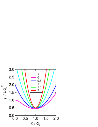
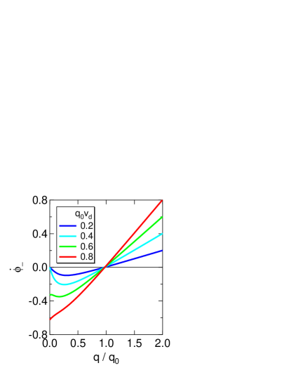
Figure 3: (Color online) The dispersion relations for (a) the decay rate and (b) the rate of phase change of the SO enhanced mode in the linear-Dresselhaus-only case. The main features resemble those in the SU(2) case, both $\gamma_{-}(q)$ show a minimum and $\dot{\phi}_{-}(q)$ vanishes at $q_{0}$, but the lifetime is finite in this case.

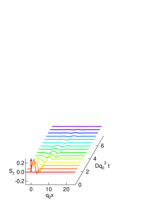
Figure 4: (Color online) The space-time evolution of $S_{z}$ in the linear-Dresselhaus-only case with the same initial condition and applied $E$ field as in the SU(2) case. The features are similar to those in the SU(2) case, except the envelope function decays exponentially.

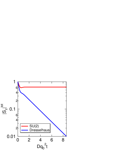
Figure 5: (Color online) The the absolute value of the spin polarization integrated over position as a function of time. In the SU(2) case, $|S_{z}|^{tot}$ is conserved after an initial decay; while in the linear-Dresselhaus-only case, $|S_{z}|^{tot}$ decays exponentially.

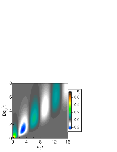
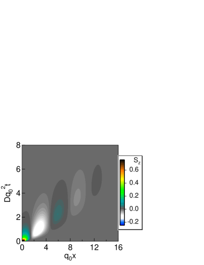
Figure 6: (Color online) The space-time images of the spin polarization in the (a) SU(2) and (b) linear-Dresselhaus-only cases, respectively.

IV Summary and conclusion

We have developed a random walk model to describe the time evolution of electron spin in two dimensions in the presence of Rashba and Dresselhaus interactions. From the random walk model we derived equations of motion for spin polarization and obtained dispersion relations for $\boldsymbol{q}$ parallel to one of the symmetry directions of the Rashba/Dresselhaus Hamiltonian. In Sec. II, we showed that the dispersion relations for spin-polarization waves that spiral in the plane containing the surface normal and the wave vector are identical to those obtained from previous analyses.SU2 ; cubic The random walk approach is instructive in showing, in a simple but explicit way, how anomalous spin diffusion and the persistent spin helix arise from nonvanishing correlations between the velocity and spin precession vectors.

In Sec. III, we obtained dispersion relations for spin-polarization waves that include the effects of an electric field parallel to $\boldsymbol{q}$, to second order in $E$. The terms linear in $E$ are equivalent to those obtained from the quantum kinetic approach.KB ; KB2 To first order in $E$, the field introduces a precession vector in the plane of the 2DEG and perpendicular to $\boldsymbol{E}$. The precession about the $y$ axis gives rise to an unusual behavior in that the spiral with wave vector $q_{0}$ is stationary in space despite the motion of electrons in the field; waves with $q>q_{0}$ propagate in the same direction as the drifting electrons while those with $q<q_{0}$ propagate “backward.” The terms that are second order in $E$ affect the decay rate of spin polarization without changing the velocity. The solutions obtained when these terms are included point to the special properties of waves with wave vector $q_{0}$, whose lifetime turns out to be unchanged by the field. However, the decay rate of the all other waves increases, in proportion to $(q-q_{0})^{2}$.

We illustrated these results by considering three representative spin-orbit Hamiltonians: SU(2) symmetric or $\alpha=\beta_{1}$ and $\beta_{3}=0$; SU(2) broken by a small but nonzero $\beta_{3}$; and linear Dresselhaus coupling only or $\alpha=\beta_{3}=0$. In order to show the nature of spin propagation more clearly, we Fourier transformed the solutions from wave vector to real space and obtained the dynamics of spin-polarization packets. In all cases the spin packets move at the electron drift velocity. In the SU(2) case the integrated amplitude of the spin spiral is conserved, while in the linear-Dresselhaus-only case the amplitude decays with a rate $\sim Dq_{0}^{2}$. When SU(2) is weakly broken by small, but nonzero $\beta_{3}$, the integrated amplitude decays at a rate $\sim(\beta_{3}/\beta_{1})^{2}Dq_{0}^{2}$.

The conclusions reached by our analysis of the RW model are consistent with a recent Monte Carlo study of a specific 2DEG system, a (001) $\hbox{In}_{1-x}\hbox{Ga}_{x}\hbox{As}$ quantum well with carrier density $\sim 10^{12}$ cm^-2 (Ref. Ohno, ). In this study spin polarization dynamics were calculated under conditions of steady state injection from a ferromagnetic contact. For $\alpha/\beta_{1}$ ratios that are close to unity, the spin polarization is conserved over several wavelengths of the PSH, despite the fact that transport takes place in the diffusive regime. Moreover, the polarization is not diminished with increasing electric field. The authors point out that the PSH effect can be used to achieve a novel variation of the Datta-Das spin-field-effect transistor (Ref. DD, ) in which a gate electrode modulates the $\alpha$ to $\beta_{1}$ ratio only slightly away from unity. This has the effect of varying the wavelength of the PSH without significantly reducing its lifetime. Thus small changes in gate voltage can in principle lead to large changes in source to drain conductance. Whether such a device can actually be realized depends on two factors: fabricating ferromagnetic injectors and analyzers with high figures of merit, and demonstrating that the PSH effects that have been observed at temperatures below $\sim$ 100 K (Ref. jake, ) can be realized at room temperature.

- (1) T. Dietl, D. D. Awschalom, M. Kaminska, and H. Ohno, Spintronics, Semiconductors and Semimetals Vol. 82 (Academic Press, New York, 2008).
- (2) J. Fabian, A. Matos-Abiague, C. Ertler, P. Stano, and I. Žutić, Acta Phys. Slov. 57, 565 (2007).
- (3) M. W. Wu, J. H. Jiang, and M. Q. Weng, Phys. Rep. 493, 61 (2010).
- (4) F. J. Ohkawa and Y. Uemura, J. Phys. Soc. Jpn. 37, 1325 (1974).
- (5) Y. A. Bychkov and E. I. Rashba, J. Phys. C 17, 6039 (1984).
- (6) Y. A. Bychkov and E. I. Rashba, JETP Lett. 39, 78 (1984).
- (7) M. I. D’yakonov and V. I. Perel’, JEPT Lett. 13, 467 (1971).
- (8) M. I. D’yakonov and V. I. Perel’, Zh. Eksp. Teor. Fiz. 60, 1954 (1971) [Sov. Phys. JETP 33, 1053 (1971)].
- (9) F. Meier and B. P. Zakharchenya, eds., Optical Orientation, vol. 8 of Modern Problems in Condensed Matter Sciences (North-Holland, 1984).
- (10) M. I. D’yakonov and V. Yu. Kachorovskii, Fiz. Tekh. Poluprovodn. 20, 178 (1986) [Sov. Phys. Semicond. 20, 110 (1986)].
- (11) G. Dresselhaus, Phys. Rev. 100, 580 (1955).
- (12) J. Schliemann, J. C. Egues, and D. Loss, Phys. Rev. Lett. 90, 146801 (2003).
- (13) B. A. Bernevig, J. Orenstein, and S.-C. Zhang, Phys. Rev. Lett. 97, 236601 (2006).
- (14) A. A. Burkov, A. S. Nunez, and A. H. MacDonald, Phys. Rev. B 70, 155308 (2004).
- (15) E. G. Mishchenko, A. V. Shytov, and B. I. Halperin, Phys. Rev. Lett. 93, 226602 (2004).
- (16) T. D. Stanescu and V. Galitski, Phys. Rev. B 75, 125307 (2007).
- (17) J. D. Koralek, C. P. Weber, J. Orenstein, B. A. Bernevig, S.-C. Zhang, S. Mack, and D. D. Awschalom, Nature (London) 458, 610 (2009).
- (18) P. Kleinert and V. V. Bryksin, Phys. Rev. B 76, 205326 (2007).
- (19) P. Kleinert and V. V. Bryksin, Phys. Rev. B 79, 045317 (2009).
- (20) M. M. Glazov and E. Y. Sherman, Phys. Rev. B 71, 241312(R) (2005).
- (21) V. K. Dugaev, E. Ya. Sherman, V. I. Ivanov, and J. Barnaś, Phys. Rev. B 80, 081301(R) (2009).
- (22) R. Winkler, Spin-Orbit Coupling Effects in Two-Dimensional Electron and Hole Systems, Springer Tracts in Modern Physics Vol. 191 (Springer, New York, 2003).
- (23) M. Ohno and K. Yoh, Phys. Rev. B 77, 045323 (2008).
- (24) S. Datta and B. Das, Appl. Phys. Lett. 56, 665 (1990).