On the interlace polynomials

Abstract

The generating function that records the sizes of directed circuit partitions of a connected 2-in, 2-out digraph $D$ can be determined from the interlacement graph of $D$ with respect to a directed Euler circuit; the same is true of the generating functions for other kinds of circuit partitions. The interlace polynomials of Arratia, Bollobás and Sorkin [J. Combin. Theory Ser. B 92 (2004) 199-233; Combinatorica 24 (2004) 567-584] extend the corresponding functions from interlacement graphs to arbitrary graphs. We introduce a multivariate interlace polynomial that is an analogous extension of a multivariate generating function for undirected circuit partitions of undirected 4-regular graphs. The multivariate polynomial incorporates several different interlace polynomials that have been studied by different authors, and its properties include invariance under a refined version of local complementation and a simple recursive definition.

Keywords. circuit partition, interlace polynomial, isotropic system, local complementation, pivoting, split graph

Mathematics Subject Classification. 05C50

1 Introduction

In order to introduce our results and the background theory in a precise way, we need to fix some definitions. A graph $G$ consists of a finite set $V(G)$ of vertices, and a finite set $E(G)$ of edges; each element of $E(G)$ is incident on one or two vertices. An edge incident on only one vertex is a loop. Two distinct vertices incident on a single edge are neighbors; the set of neighbors of a vertex $v$ is the open neighborhood $N_{G}(v)$. It is often convenient to think of an edge as consisting of two distinct half-edges, each of which is incident on precisely one vertex. An edge is directed by specifying that one half-edge is initial and the other is terminal; as the half-edges are distinct, every edge can be directed in two different ways. The degree of a vertex $v$ is the number of half-edges incident at $v$. A $k$-regular graph is one whose vertices all have degree $k$. Edges incident on precisely the same vertices are parallel, and a graph with no loops and no parallels is simple. A circuit in a graph is a sequence $v_{1}$, $h_{1}$, $h_{2}^{\prime}$, $v_{2}$, …, $v_{k}$, $h_{k}$, $h_{k+1}^{\prime}$, $v_{k+1}=v_{1}$ such that for each $i$, $h_{i}$ and $h_{i}^{\prime}$ are half-edges incident on $v_{i}$, and $h_{i}$ and $h_{i+1}^{\prime}$ are half-edges of a single edge $e_{i}$. A vertex may appear repeatedly on a circuit, but an edge may not appear more than once. If it happens that for every $i$, $e_{i}$ is a directed edge with initial half-edge $h_{i}$, then the circuit is directed; in general a directed graph may contain both directed circuits and undirected circuits. An Eulerian graph is a graph that possesses at least one Eulerian circuit, i.e., a circuit which includes every edge.

This paper concerns a family of graph invariants, the interlace polynomials. We use the term in a generic sense, to include also some polynomials that were introduced under other names. All of these polynomials are motivated by the circuit theory of 4-regular graphs.

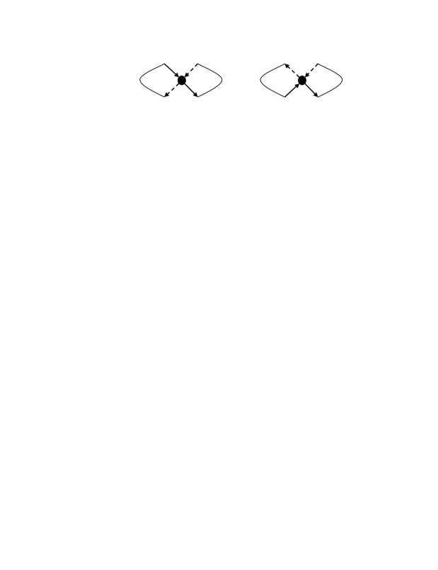
Figure 1: $C\ast v$ is obtained by reversing either of the two $v$-to-$v$ walks within the incident circuit of $C$.

Four cornerstones of this theory were laid in the 1960s and 1970s. A connected 4-regular graph is Eulerian, of course. More generally, an arbitrary 4-regular graph has Euler systems, each of which contains one Euler circuit for each connected component of the graph. Kotzig [47] introduced the $\kappa$-transformations: if $C$ is an Euler system of a 4-regular graph $F$ and $v\in V(F)$ then the $\kappa$-transform $C\ast v$ is the Euler system obtained from $C$ by reversing one of the two $v$-to-$v$ walks within the circuit of $C$ incident on $v$. Kotzig’s theorem is the first of the four cornerstones; it tells us that all the Euler systems of $F$ can be obtained from any one using $\kappa$-transformations.

Although our discussion is focused on 4-regular graphs, we should certainly mention that Kotzig’s theorem extends to arbitrary Eulerian graphs; see Fleischner’s books [31, 32] for an account of the general theory.

The second cornerstone of the circuit theory of 4-regular graphs is the interlacement graph $\mathcal{I}(F,C)$ of a 4-regular graph with respect to an Euler system $C$. $\mathcal{I}(F,C)$ is the simple graph with the same vertices as $F$, in which two vertices $v$ and $w$ are neighbors if and only if they are interlaced with respect to $C$, i.e., they appear in the order $v...w...v...w$ on one of the circuits of $C$. The graphs that arise as interlacement graphs are called circle graphs. (This definition is usually restricted to Euler circuits of connected 4-regular graphs, but the restriction would be inconvenient here because there are natural ways to recursively simplify 4-regular graphs, which sometimes disconnect them.) This construction was discussed by Bouchet [11] and Read and Rosenstiehl [59], who observed that the relationship between $\mathcal{I}(F,C)$ and $\mathcal{I}(F,C\ast v)$ is described by simple local complementation at $v$: if $v\neq x\neq y\neq v$ and $x,y$ are both neighbors of $v$ in $F$ then $x$ and $y$ are adjacent in $\mathcal{I}(F,C\ast v)$ if and only if they are not adjacent in $\mathcal{I}(F,C)$. Later, Bouchet introduced isotropic systems to study circle graphs and the equivalence relation on arbitrary graphs generated by simple local complementations [13, 14, 15, 17].

By the way, we use the term simple local complementation to distinguish this operation from the one that Arratia, Bollobás and Sorkin called local complementation in [2, 3, 4]; that operation also includes loop-toggling at neighbors of $v$.

If $C$ is an Euler system of $F$, then $F$ is made into a 2-in, 2-out digraph $D$ by choosing either of the two orientations for each circuit of $C$, and directing the edges of $F$ accordingly. If $v$ and $w$ are neighbors in $\mathcal{I}(F,C)$ then the iterated $\kappa$-transform $C\ast v\ast w\ast v$ is also a directed Euler system for $D$, obtained by interchanging the two $v$-to-$w$ walks within the incident circuit of $C$. Following [2, 3], we refer to the operation $C\mapsto C\ast v\ast w\ast v$ as transposition; the induced operation on interlacement graphs is pivoting, denoted $G\mapsto G^{vw}$. Kotzig [47], Pevzner [58] and Ukkonen [72] proved that transpositions suffice to obtain all the directed Euler systems for a 2-in, 2-out digraph from any one; a more general form of this theorem was proven by Fleischner, Sabidussi, and Wenger [33].

Figure 2: $D_{1}$ (top left) and $D_{2}$ (bottom left) are nonisomorphic directed graphs whose undirected versions are isomorphic. They yield interlacement graphs that are equivalent under local complementation but not under pivoting.

As examples of these notions, consider the 2-in, 2-out digraphs $D_{1}$ and $D_{2}$ of Figure 2. They are small enough so that each has only one directed Euler circuit, up to automorphism. Two Euler circuits are indicated in the figure; to trace an Euler circuit follow the directed edges, making sure to maintain the same dash pattern when traversing a vertex. (The dash pattern may be changed while traversing an edge.) The corresponding interlacement graphs are indicated in the figure’s third column. Pivoting on an edge in the lower interlacement graph produces an isomorphic replica, with a different degree-2 vertex; pivoting on an edge in the upper interlacement graph has no effect at all. The fact that the two interlacement graphs are not equivalent under pivoting reflects the fact that $D_{1}$ and $D_{2}$ are not isomorphic. On the other hand, simple local complementation at the single degree-2 vertex of the lower interlacement graph produces the upper interlacement graph, reflecting the fact that the undirected versions of $D_{1}$ and $D_{2}$ are isomorphic.

Let $F$ be a 4-regular graph with $c(F)$ connected components, and let $C$ be an Euler system of $F$. A circuit partition or Eulerian partition of $F$ is a partition of $E(F)$ into edge-disjoint circuits. Such a partition is determined by choosing, at each vertex of $F$, one of the three transitions (pairings of the incident half-edges): the transition that appears in the incident circuit of $C$, which we label $\phi$, for “follow”; the other transition consistent with the edge-directions given by the incident circuit of $C$, which we label $\chi$, for “cross”; or the transition that is inconsistent with these edge-directions, which we label $\psi$. See Figure 3. (We should mention that we use the terminology of Ellis-Monaghan and Sarmiento [29] and Jaeger [41], in which a transition at $v$ specifies both pairings of incident half-edges that might appear in a circuit partition. Other authors, including Bouchet and Kotzig, use “transition” in a slightly different way, to refer to a single pairing of half-edges, and require a separate matching-up of the pairings.) If $n=\left|V(F)\right|$ then $F$ has $3^{n}$ circuit partitions, given by choosing one of the three transitions at each vertex. A 2-in, 2-out digraph has $2^{n}$ directed circuit partitions.

Figure 3: An orientation of the circuit of $C$ incident at $v$ is indicated at left. Each circuit partition of $F$ involves one of the three pictured transitions at $v$. Both orientations of the incident circuit of $C$ result in the same labeling of these three transitions.

The third cornerstone of the circuit theory of 4-regular graphs is the idea of defining a polynomial invariant of a 2-in, 2-out digraph (or 4-regular graph) by using some form of the generating function $\sum x^{\left|P\right|}$ that records the sizes of (un)directed circuit partitions. This idea was introduced by Las Vergnas [51], who observed that a polynomial defined recursively by Martin [54] is essentially equivalent to the generating function. Las Vergnas also extended the idea to general Eulerian graphs, and to 4-regular graphs that arise as medial graphs imbedded in the projective plane and the torus [49, 50]. In particular, if a 4-regular graph $F$ is imbedded in the plane then its complementary regions can be colored checkerboard fashion, yielding a pair of dual graphs with $F$ as medial, and the Tutte polynomial of either of the two dual graphs yields the directed circuit partition generating function for a certain directed version of $F$; this theorem foreshadowed the famous connection between the Tutte polynomial and the Jones polynomial of knot theory [42, 44, 63]. We will not focus any further attention on imbedded graphs in this paper; we refer the interested reader to Ellis-Monaghan and Moffatt [28] for a thorough discussion including recent results.

Martin observed that the circuit partition generating functions can be described recursively. Suppose $F$ is a 4-regular graph with an Euler system $C$, $D$ is the 2-in, 2-out digraph corresponding to a choice of orientations for the circuits of $C$, and $v$ is unlooped in $F$. The directed circuit partitions of $D$ fall into two classes, those that follow $C$ through $v$ and those that involve the $\chi$ transition at $v$. These two classes correspond to directed circuit partitions of the two digraphs $D_{\phi}$ and $D_{\chi}$ obtained by directed detachment at $v$, illustrated in Figure 4. (The term detachment was coined by Nash-Williams; see [57] for instance.)

Figure 4: The two digraphs obtained by directed detachment at $v$.

Similarly, the circuit partitions of $F$ fall into three classes according to the transitions at $v$, and the three classes correspond to circuit partitions of three graphs $F_{\phi}$, $F_{\chi}$ and $F_{\psi}$ obtained by detachment at $v$.

The fourth cornerstone involves an equality due to Cohn and Lempel [22]. In its original form, the equality relates the number of cycles in a permutation to the nullity of an associated skew-symmetric matrix over $GF(2)$. An equivalent form of the equality relates the number of circuits in a directed circuit partition of a connected 2-in, 2-out digraph $D$ to the nullity of the adjacency matrix of an associated subgraph of an interlacement graph $\mathcal{I}(D,C)$. It is remarkable that versions of this useful equality have been discovered and rediscovered by combinatorialists and topologists so many times [6, 8, 12, 19, 40, 43, 46, 52, 53, 55, 56, 60, 61, 62, 73]. The Cohn-Lempel equality extends to a circuit-nullity formula for undirected circuit partitions in undirected 4-regular graphs. We simply state the formula here, and refer to [66, 70] for more detailed accounts. Let $G=\mathcal{I}(F,C)$, let $P$ be a circuit partition of $F$, and let $G_{P}=\mathcal{I}_{P}(F,C)$ be the graph obtained from $G$ by removing each vertex at which $P$ involves the $\phi$ transition used by $C$, and attaching a loop at each vertex where $P$ involves the $\psi$ transition. Then the circuit-nullity formula states that

$$\left|P\right|-c(F)=\nu(G_{P}),$$

where $\nu(G_{P})$ denotes the $GF(2)$-nullity of the adjacency matrix of $G_{P}$, i.e., the difference between $\left|V(G_{P})\right|$ and the $GF(2)$-rank. (The adjacency matrix of $G_{P}$ is the $V(G_{P})\times V(G_{P})$ matrix over $GF(2)$ in which a diagonal entry is nonzero if and only if the corresponding vertex is looped, and an off-diagonal entry is nonzero if and only if the two corresponding vertices are neighbors.) The original Cohn-Lempel equality is essentially the special case in which $c(F)=1$ and no $\psi$ transition appears in $P$.

Figure 5: Three circuit partitions $P_{1},P_{2},P_{3}$ in the 4-regular graph of Figure 2, with the transition labels and $G_{P}$ graphs corresponding to the two Euler circuits shown there.

Some examples appear in Figure 5. Three circuit partitions $P_{1},P_{2},P_{3}$ of the undirected version of the graphs $D_{1}$ and $D_{2}$ of Figure 2 are depicted in the top row. Each circuit is traced out by maintaining the dash pattern when traversing a vertex; the dash pattern may change when traversing an edge, though. Transition labels indicate the relationships between these circuit partitions and the Euler circuit of $D_{1}$ indicated in Figure 2. The corresponding graphs $G_{P_{i}}$ appear in the second row. In the third row of Figure 5 we see the same three circuit partitions, now with transition labels that indicate their relationships with the Euler circuit of $D_{2}$ indicated in Figure 2. The corresponding graphs $G_{P_{i}}$ appear in the fourth row. The circuit-nullity formula is satisfied because both sets of graphs $G_{P_{i}}$ satisfy $\nu(G_{P_{1}})=2=3-1$, $\nu(G_{P_{2}})=1=2-1$ and $\nu(G_{P_{3}})=0=1-1$.

If $F$ is a 4-regular graph with an Euler system $C$, then the circuit-nullity formula provides a bijective equivalence between these two information-sets.

1. List the circuit partitions of $F$; for each circuit partition, specify the corresponding choice of the $\phi,\chi$ or $\psi$ transition at each vertex, and also the number of circuits.

2. List the looped full subgraphs of $\mathcal{I}(F,C)$; for each looped full subgraph, specify the corresponding decision to remove, retain or loop each vertex, and also the $GF(2)$-nullity of the adjacency matrix.

This bijective equivalence tells us that the generating functions that record the sizes of (un)directed circuit partitions in $F$ – or equivalently, the Martin polynomials – can be reformulated as generating functions that record the binary nullities of adjacency matrices of (looped) full subgraphs of $\mathcal{I}(F,C)$. Observe that there is no reason the nullity-based reformulations of these generating functions should be restricted to interlacement graphs; the definitions extend unchanged to arbitrary simple graphs. The graph polynomial that extends the directed Martin polynomial, the (vertex-nullity) interlace polynomial $q_{N}(G)$, was introduced by Arratia, Bollobás and Sorkin [2, 3]. Their original definition extended the recursive description of the Martin polynomial, rather than the nullity-based reformulation; they derived the nullity-based form in [4], where they also introduced a two-variable interlace polynomial $q(G)$. Subsequently, Aigner and van der Holst [1] defined another interlace polynomial $Q(G)$, which extends the reformulated version of the undirected Martin polynomial. More recently, Courcelle [26] introduced a multivariate interlace polynomial $C(G)$, which extends a logically equivalent form of the information described in item 2 above. These graph polynomials are related in various ways to the (un)restricted “Tutte-Martin polynomials” of isotropic systems studied by Bouchet [16, 18].

Our purpose in the present paper is to incorporate the $\phi,\chi,\psi$ labels into the machinery outlined above. This is accomplished in two stages. In Section 2, $\phi,\chi$ and $\psi$ are introduced into the circuit theory of 4-regular graphs as transition labels. These transition labels are neither absolute nor arbitrary; they are defined with respect to a particular Euler system, and they are modified in particular ways when $\kappa$-transformations are applied to that Euler system. The labeled versions of the Martin polynomials are generating functions that record the sizes of (un)directed circuit partitions, along with the corresponding transition labels. (The $\psi$ label is not needed for directed circuit partitions.) These labeled versions of the Martin polynomials are specializations of the transition polynomials discussed by Jaeger [41] and Ellis-Monaghan and Sarmiento [29]; the transition polynomials also incorporate transition labels, but the labels are arbitrary and consequently carry less information than $\phi,\chi$ and $\psi$.

The equivalence between items 1 and 2 above tells us that the labeled versions of the (un)directed Martin polynomials can be reformulated as labeled generating functions that record the $GF(2)$-nullities of adjacency matrices of (looped) full subgraphs of interlacement graphs. In Sections 3 – 5, these generating functions are extended from labeled interlacement graphs to general labeled graphs, with vertex labels $\phi,\chi,\psi$ now representing three ways to treat a vertex (remove it, retain it, or attach a loop) rather than three ways to choose a transition. The result is to unify all the polynomial invariants of graphs and isotropic systems discussed in the paragraph before last in a single multivariate graph polynomial, the labeled interlace polynomial $Q_{\lambda}(G)$, whose properties include a three-term recursive definition and invariance under labeled local complementation. Setting $\psi\equiv 0$ in $Q_{\lambda}(G)$ we obtain the 2-label interlace polynomial $q_{\lambda}(G)$, which extends the nullity-based reformulation of the directed Martin polynomial. It satisfies a two-term recursion and is invariant under labeled pivoting.

In Section 6 we detail the relationships between $Q_{\lambda}$ and the several kinds of interlace polynomials that have been studied since the original definition of Arratia, Bollobás and Sorkin [2, 3, 4]. In Section 7 we present formulas for the labeled interlace polynomials of graphs with split decompositions, and discuss their computational significance.

Acknowledgments. Before proceeding to present these notions in detail, we should thank D. P. Ilyutko, V. O. Manturov and L. Zulli. The idea of using label-switching local complementations was inspired by many conversations with them while we studied the use of interlacement to describe the Jones polynomial and Kauffman bracket of a link diagram [37, 38, 39, 65, 67, 68, 71]. Preliminary drafts of the paper were significantly improved by the kind advice of B. Bollobás, B. Courcelle, J. A. Ellis-Monaghan, C. Hoffmann, M. Las Vergnas and an anonymous reader.

2 Transition labels and circuit partitions

Definition 1

An Euler system $C$ in a 4-regular graph $F$ is labeled by giving a trio of functions $\phi_{C}$, $\chi_{C}$, $\psi_{C}$ mapping $V(F)$ into some commutative ring $R$.

When we want to specify the ring in question, we refer to $C$ as $R$-labeled. We will see in Section 6 that it is useful to consider a variety of labeling strategies, in a variety of rings. However, there is an especially natural way to implement Definition 1. Suppose $R$ is a polynomial ring with $3\cdot\left|V(F)\right|$ indeterminates, one indeterminate corresponding to each transition at each vertex of $F$. For each $v\in V(F)$, define the images of $v$ under $\phi_{C}$, $\chi_{C}$, and $\psi_{C}$ in accordance with Figure 3. Then the label function $\phi_{C}$ actually specifies the Euler system $C$.

Recall that a $\kappa$-transformation is applied by reversing one of the two $v$-to-$v$ walks in an Euler system, as depicted in Figure 1. Clearly this reversal affects some transition labels: at $v$ itself, the $\phi$ and $\psi$ labels are interchanged; and at a vertex $w$ that appears precisely once on the reversed $v$-to-$v$ walk, the $\chi$ and $\psi$ labels are interchanged.

Definition 2

Let $v$ be a vertex of a 4-regular graph $F$, and let $C$ be a labeled Euler system of $F$. The labeled $\kappa$-transform $C\ast v$ is obtained by reversing one of the two $v$-to-$v$ walks within the circuit of $C$ incident on $v$, and making the following label changes: $\phi_{C\ast v}(v)=\psi_{C}(v)$, $\psi_{C\ast v}(v)=\phi_{C}(v)$, and for each $w$ that neighbors $v$ in $\mathcal{I}(F,C)$, $\chi_{C\ast v}(w)=\psi_{C}(w)$ and $\psi_{C\ast v}(w)=\chi_{C}(w)$.

Definition 3

Two labeled Euler systems of a 4-regular graph are $\kappa$-equivalent if and only if one can be obtained from the other through labeled $\kappa$-transformations.

Kotzig’s theorem [47] tells us that $\kappa$-transformations can be used to obtain all the Euler systems of $F$ from any one; it follows that if $F$ has Euler systems $C_{1}$ and $C_{2}$ then each labeled version of $C_{1}$ is $\kappa$-equivalent to a unique labeled version of $C_{2}$.

Definition 4

Let $C$ be an $R$-labeled Euler system of $F$, and suppose $y\in R$. For each circuit partition $P$ of $F$, let $\phi(P,C)$, $\chi(P,C)$ and $\psi(P,C)$ denote the sets of vertices of $F$ where $P$ involves the transition labeled $\phi$, $\chi$ or $\psi$ (respectively) with respect to $C$. The $R$-labeled circuit partition generating function of $F$ with respect to $C$ is

$$\pi(F,C)=\sum_{P\in\mathcal{P}(F)}\left({\displaystyle\prod_{v\in\phi(P,C)}}\phi_{C}(v)\right)\left({\displaystyle\prod_{v\in\chi(P,C)}}\chi_{C}(v)\right)\left({\displaystyle\prod_{v\in\psi(P,C)}}\psi_{C}(v)\right)y^{\left|P\right|-c(F)},$$

where $\mathcal{P}(F)$ is the set of circuit partitions of $F$ and $c(F)$ is the number of connected components of $F$.

Different systems of labels yield generating functions with different levels of detail. If the labels take the natural values in the polynomial ring $\mathbb{Z}[\{y\}\cup\{\phi_{C}(v),\chi_{C}(v),\psi_{C}(v)$ $|$ $v\in V(F)\}]$ with $1+3\cdot\left|V(F)\right|$ independent indeterminates, then $\pi(F,C)\,$ is essentially a table that lists, for every circuit partition $P$, $\left|P\right|-c(F)$ along with the relationship between $C$ and $P$ at every vertex. Similarly, the $\psi\equiv 0$ specialization of this polynomial is essentially a generating function for directed circuit partitions of a 2-in, 2-out digraph $D$ obtained by directing the edges of $F$ according to orientations of the circuits of $C$. The theory of this polynomial is outlined in Section 5. If $\phi,\chi,\psi\equiv 1\in\mathbb{Z}[y]$ then $\pi(F,C)$ is the ordinary (unlabeled) generating function for circuit partitions of $F$, and if $\psi\equiv 0$ and $\phi,\chi\equiv 1\in\mathbb{Z}[y]$ then $\pi(F,C)$ is the ordinary generating function for circuit partitions of $D$.

Proposition 5

Let $C_{1}$ and $C_{2}$ be labeled Euler systems in $F$. If $C_{1}$ and $C_{2}$ are $\kappa$-equivalent, then $\pi(F,C_{1})=\pi(F,C_{2})$.

Proof. Labeled $\kappa$-transformations preserve $\pi$ term by term, because the contribution of each $P\in\mathcal{P}(F)$ is unchanged.   

The labeled circuit partition generating function $\pi(F,C)$ incorporates more precise information about the structure of a 4-regular graph $F$ than other transition-based polynomials that have appeared in the literature. For instance, the “Tutte-Martin polynomials” discussed by Bouchet [16] involve “coding” each vertex of $F$ by choosing an arbitrary labeling of the transitions. (Indeed Proposition (5.2) of [13] states that the isotropic systems associated to two coded 4-regular graphs are isomorphic if and only if they can be obtained from differently coded versions of the same 4-regular graph.) Jaeger’s transition polynomial [41] and the generalized transition polynomial of Ellis-Monaghan and Sarmiento [30] also involve arbitrary transition labels. In contrast, the label functions $\phi_{C}$, $\chi_{C}$ and $\psi_{C}$ are not arbitrary: they are associated in special ways with the positioning of $C$ within $F$, and they are handled in special ways by labeled $\kappa$-transformations.

In particular, it is not generally possible to simply transpose two labels at one vertex using labeled $\kappa$-transformations. For example, suppose $C$ is any labeled Euler circuit of the graph $F$ in Figure 6, with 21 independent indeterminates serving as transition labels (three for each vertex). Then $\pi(F,C)$ determines the $\chi$ labels at the two central vertices of the graph: they are the only transition labels that appear only in terms divisible by $y$, because the corresponding transitions are the only ones that do not appear in any Euler circuit. Similarly, if $F_{1}$ is the undirected version of the graph $D_{1}$ of Figure 2, and $C_{1}$ is the Euler circuit of $D_{1}$ indicated in Figure 2, then the $\psi$ labels in $F_{1}$ are distinguished by the fact that they are the only ones that appear in a term of $\pi(F_{1},C_{1})$ divisible by $y^{3}$.

Figure 6: All Euler circuits have the same $\chi$ transitions at the central vertices.

The labeled circuit partition generating function $\pi(F,C)$ satisfies a labeled version of the detachment-based recursion mentioned in the introduction. Suppose $C$ is a labeled Euler system of $F$ and $v$ is an unlooped vertex of $F$. (We leave the consideration of looped vertices to the reader.) Then as discussed in the introduction, there are three associated 4-regular graphs obtained by detachment at $V$, denoted $F_{\phi}$, $F_{\chi}$ and $F_{\psi}$ according to the transitions that define the detachments. As illustrated in Figure 7, $C$ yields labeled Euler systems in all three detachments. $F_{\phi}$ has a labeled Euler system $C_{\phi}$ whose circuits simply follow the circuits of $C$, omitting $v$. $F_{\psi}$ has a labeled Euler system $C_{\psi}$, obtained in the same way from the labeled $\kappa$-transform $C\ast v$. The situation in $F_{\chi}$ is more complicated, as there are two distinct cases. If $v$ is not interlaced with any other vertex with respect to $C$, then $c(F_{\chi})=c(F)+1$ and $F_{\chi}$ has a labeled Euler system $C_{\chi}$ obtained by separating the two $v$-to-$v$ circuits within the incident circuit of $C$. On the other hand if $v$ is interlaced with a vertex $w$, then $c(F_{\chi})=c(F)$ and a labeled Euler system $C_{\chi}$ of $F_{\chi}$ is obtained by following the circuits of $C\ast w\ast v\ast w$, omitting $v$.

Figure 7: The graph of Figure 6 appears on the left, with an Euler circuit indicated by dashes. The top row depicts the three detachments at a central vertex and the bottom row depicts the three detachments at another vertex.

Theorem 6

Suppose $v$ is an unlooped vertex of $F$. Then

$$\pi(F,C)=\phi_{C}(v)\cdot\pi(F_{\phi},C_{\phi})+\chi_{C}(v)\cdot\pi(F_{\chi},C_{\chi})+\psi_{C}(v)\cdot\pi(F_{\psi},C_{\psi}).$$

Proof. The formula is justified in the natural way, by classifying the circuit partitions of $F$ according to the transitions at $v$. The notation $(F_{\chi},C_{\chi})$ is ambiguous – it does not tell us whether the first case or the second case holds in $F$, and in the second case it does not reflect the fact that different choices of $w$ will yield different labeled Euler systems in $F_{\chi}$ – but this ambiguity does no harm because the formula holds for every choice of $C_{\chi}$.   

3 Vertex labels and partitions

As discussed in the introduction, the circuit-nullity formula allows us to reformulate the theory described in Section 2: rather than thinking of circuit partitions in a 4-regular graph $F$, we may think of graphs obtained from an interlacement graph $\mathcal{I}(F,C)$ by removing some vertices and looping some vertices. This reformulated version of the theory extends directly from interlacement graphs to arbitrary simple graphs.

Definition 7

A simple graph $G$ is ($R$-)labeled by giving a trio of functions $\phi_{G}$, $\chi_{G}$, $\psi_{G}$ mapping $V(G)$ into some commutative ring $R$.

Once again, the most natural ring to use as $R$ is a polynomial ring with three independent indeterminates $\phi_{G}(v)$, $\chi_{G}(v)$ and $\psi_{G}(v)$ for each $v\in V(G)$.

Definition 8

Let $G$ be a labeled simple graph with a vertex $v$. The labeled local complement $G_{\lambda}^{v}$ is the labeled graph obtained from $G$ by toggling adjacencies between distinct neighbors of $v$ and making the following label changes: $\phi_{G_{\lambda}^{v}}(v)=\psi_{G}(v)$, $\psi_{G_{\lambda}^{v}}(v)=\phi_{G}(v)$, and for each $w$ that neighbors $v$ in $G$, $\chi_{G_{\lambda}^{v}}(w)=\psi_{G}(w)$ and $\psi_{G_{\lambda}^{v}}(w)=\chi_{G}(w)$.

Recall Definition 2: if $C$ is a labeled Euler system in a 4-regular graph $F$, then for $v\in V(F)$ the labeled $\kappa$-transform $C\ast v$ is obtained by reversing one of the two $v$-to-$v$ walks within the circuit of $C$ incident on $v$, and making appropriate adjustments to the label functions. The effect of reversing a $v$-to-$v$ walk is to toggle interlacements between vertices that appear precisely once on that walk, i.e., vertices that are interlaced with $v$. We conclude the following.

Theorem 9

Let $F$ be a 4-regular graph with a labeled Euler system $C$, and consider $\mathcal{I}(F,C)$ and $\mathcal{I}(F,C\ast v)$ as labeled graphs with the trios of label functions $\phi_{C}$, $\chi_{C}$, $\psi_{C}$ and $\phi_{C\ast v}$, $\chi_{C\ast v}$, $\psi_{C\ast v}$ (respectively). Then $\mathcal{I}(F,C\ast v)=\mathcal{I}(F,C)_{\lambda}^{v}$.

We now have three different kinds of local complementation: simple local complementation, for which we use no particular symbol; the local complementation $G^{v}$ used by Arratia, Bollobás and Sorkin [2, 3, 4], which combines simple local complementation with loop-toggling at neighbors of $v$; and labeled local complementation. The loop-toggling at neighbors of $v$ in $G^{v}$ and the $\chi\leftrightarrow\psi$ exchange at neighbors of $v$ in $G_{\lambda}^{v}$ are essentially the same thing; what is special about labeled local complementation is the $\phi\leftrightarrow\psi$ exchange at $v$ itself. As we show in Theorems 13 and 16 below, this detail allows us to formulate a simple invariance property for a rather complicated-seeming graph polynomial that determines all the different interlace polynomials studied in [1, 2, 3, 4, 16, 18, 26]. It is the absence of this detail that creates the seeming lack of simple invariance properties in the original discussions of some of these graph polynomials.

The reformulated version of a circuit partition is a certain kind of vertex partition.

Definition 10

A labeled partition of a labeled simple graph $G$ is a partition $P$ of $V(G)$ into three pairwise disjoint subsets, $V(G)=\phi(P)\cup\chi(P)\cup\psi(P)$. The set of all labeled partitions of $G$ is denoted $\mathcal{P}_{\lambda}(G)$.

Note the different uses of the term “labeled” in Definitions 7 and 10: a graph is labeled by specifying functions $\phi_{G}$, $\chi_{G}$ , $\psi_{G}:V(G)\rightarrow R$, but a partition $P$ of $V(G)$ into three disjoint subsets is labeled by identifying one of the subsets as $\phi(P)$, another as $\chi(P)$, and the third as $\psi(P)$.

Definition 11

If $v\in V(G)$ then the labeled local complement of $P\in\mathcal{P}_{\lambda}(G)$ is the labeled partition $P_{\lambda}^{v}\in\mathcal{P}(G_{\lambda}^{v})$ obtained from $P$ by making the following changes: $v\in\phi(P_{\lambda}^{v})$ if and only if $v\in\psi(P)$, $v\in\psi(P_{\lambda}^{v})$ if and only if $v\in\phi(P)$, and if $w$ is a neighbor of $v$ in $G$ then $w\in\chi(P_{\lambda}^{v})$ if and only if $w\in\psi(P)$, and $w\in\psi(P_{\lambda}^{v})$ if and only if $w\in\chi(P)$.

The circuit-nullity formula suggests the following.

Definition 12

If $P$ is a labeled partition of a simple graph $G$ then $G_{P}$ denotes the graph obtained from $G$ by removing every vertex in $\phi(P)$ and attaching a loop at every vertex in $\psi(P)$.

If $P$ is a circuit partition of a 4-regular graph $F$ with two Euler systems $C_{1}$ and $C_{2}$, then the circuit-nullity formula tells us that $\left|P\right|$ is related to the binary nullities of the adjacency matrices of the two $G_{P}$ graphs obtained from $\mathcal{I}(F,C_{1})$ and $\mathcal{I}(F,C_{2})$. $P$ itself does not change when we change Euler system, so these two adjacency matrices must have the same nullity. It may be a surprise that this invariance of nullity extends to arbitrary graphs, even though there is no fixed object that plays the role of $P$.

Theorem 13

If $v\in V(G)$ then for every $P$ in $\mathcal{P}_{\lambda}(G)$, we have $\nu(G_{P})=\nu((G_{\lambda}^{v})_{P_{\lambda}^{v}})$.

Proof. If $v\in\phi(P)$, the theorem states that

$$\left(\begin{array}[c]{ccc}M_{11}&M_{12}&M_{13}\\ M_{21}&M_{22}&M_{23}\\ M_{31}&M_{32}&M_{33}\end{array}\right)\text{ and }\left(\begin{array}[c]{cccc}1&\mathbf{1}&\mathbf{1}&\mathbf{0}\\ \mathbf{1}&\overline{M}_{11}&\overline{M}_{12}&M_{13}\\ \mathbf{1}&\overline{M}_{21}&\overline{M}_{22}&M_{23}\\ \mathbf{0}&M_{31}&M_{32}&M_{33}\end{array}\right)$$

have the same $GF(2)$-nullity. Here the left-hand matrix is partitioned into sets of rows and columns corresponding respectively to the neighbors of $v$ in $\chi(P)$, the neighbors of $v$ in $\psi(P)$, and the vertices in $\chi(P)\cup\psi(P)$ that are not neighbors of $v$; the first row and column of the right-hand matrix correspond to $v$. Bold numerals denote rows and columns with all entries the same, and an overbar indicates the toggling of all entries in a matrix over $GF(2)$. The nullity equality is verified by observing that adding the first row to every row in the first two sets of rows in the right-hand matrix yields

$$\left(\begin{array}[c]{cccc}1&\mathbf{1}&\mathbf{1}&\mathbf{0}\\ \mathbf{0}&M_{11}&M_{12}&M_{13}\\ \mathbf{0}&M_{21}&M_{22}&M_{23}\\ \mathbf{0}&M_{31}&M_{32}&M_{33}\end{array}\right),$$

whose nullity is the same is that of the first matrix displayed above.

If $v\in\psi(P)$ the preceding argument is simply reversed. That is, we use row operations to show that

$$\left(\begin{array}[c]{cccc}1&\mathbf{1}&\mathbf{1}&\mathbf{0}\\ \mathbf{1}&M_{11}&M_{12}&M_{13}\\ \mathbf{1}&M_{21}&M_{22}&M_{23}\\ \mathbf{0}&M_{31}&M_{32}&M_{33}\end{array}\right)\text{ and }\left(\begin{array}[c]{ccc}\overline{M}_{11}&\overline{M}_{12}&M_{13}\\ \overline{M}_{21}&\overline{M}_{22}&M_{23}\\ M_{31}&M_{32}&M_{33}\end{array}\right)$$

have the same $GF(2)$-nullity.

If $v\in\chi(P)$ then the theorem states that

$$\left(\begin{array}[c]{cccc}0&\mathbf{1}&\mathbf{1}&\mathbf{0}\\ \mathbf{1}&M_{11}&M_{12}&M_{13}\\ \mathbf{1}&M_{21}&M_{22}&M_{23}\\ \mathbf{0}&M_{31}&M_{32}&M_{33}\end{array}\right)\text{ and }\left(\begin{array}[c]{cccc}0&\mathbf{1}&\mathbf{1}&\mathbf{0}\\ \mathbf{1}&\overline{M}_{11}&\overline{M}_{12}&M_{13}\\ \mathbf{1}&\overline{M}_{21}&\overline{M}_{22}&M_{23}\\ \mathbf{0}&M_{31}&M_{32}&M_{33}\end{array}\right)\text{ }$$

have the same $GF(2)$-nullity. This is verified by adding the first row to those in the second and third sets.   

Here is the reformulated version of Definition 4.

Definition 14

Let $G$ be an $R$-labeled simple graph, and suppose $y\in R$. The labeled interlace polynomial of $G$ is the sum

$$Q_{\lambda}(G)=\sum_{P\in\mathcal{P}_{\lambda}(G)}\left({\displaystyle\prod_{v\in\phi(P)}}\phi_{G}(v)\right)\left({\displaystyle\prod_{v\in\chi(P)}}\chi_{G}(v)\right)\left({\displaystyle\prod_{v\in\psi(P)}}\psi_{G}(v)\right)y^{\nu(G_{P})}.$$

Note that we call $Q_{\lambda}$ a polynomial even though $y$ is an arbitrary element of $R$. This is a mere formality, as we could specify that $y$ be an indeterminate and then obtain other instances of the definition through evaluation.

Theorem 15

Let $F$ be a 4-regular graph with a labeled Euler system $C$, and let $\mathcal{I}(F,C)$ be the corresponding labeled interlacement graph. Then

$$\pi(F,C)=Q_{\lambda}(\mathcal{I}(F,C)).$$

As we mentioned in the introduction, the labeled interlace polynomial yields all the different kinds of interlace polynomials in the literature, by using different label values. This might suggest that the properties of $Q_{\lambda}$ would be more complicated than those of the other polynomials; instead the theory of $Q_{\lambda}$ turns out to be considerably simpler.

Theorem 16

Let $G$ be a labeled simple graph with a vertex $v$. Then $Q_{\lambda}(G)=Q_{\lambda}(G_{\lambda}^{v})$.

Proof. This follows immediately from Theorem 13 and the fact that for every $P\in\mathcal{P}_{\lambda}(G)$,

$$\left({\displaystyle\prod_{v\in\phi(P)}}\phi_{G}(v)\right)\left({\displaystyle\prod_{v\in\chi(P)}}\chi_{G}(v)\right)\left({\displaystyle\prod_{v\in\psi(P)}}\psi_{G}(v)\right)$$

$$=\left({\displaystyle\prod_{v\in\phi(P_{\lambda}^{v})}}\phi_{G_{\lambda}^{v}}(v)\right)\left({\displaystyle\prod_{v\in\chi(P_{\lambda}^{v})}}\chi_{G_{\lambda}^{v}}(v)\right)\left({\displaystyle\prod_{v\in\psi(P_{\lambda}^{v})}}\psi_{G_{\lambda}^{v}}(v)\right).$$

 

How can it be that $Q_{\lambda}$ is invariant under labeled local complementation, when choosing particular labels in $Q_{\lambda}$ yields the multivariable interlace polynomials of [4] and [26], which seem to have no invariance properties at all? The answer is given in Section 6 below: the choices of labels that yield these polynomials do not maintain the separation of $\phi$, $\chi$ and $\psi$. Losing this three-fold distinction makes it impossible to apply Definition 8, and consequently the properties of $Q_{\lambda}$ are obscured.

Theorem 17

The labeled interlace polynomial of a labeled simple graph is recursively determined by these three properties.

1. If $G$ consists only of a single vertex $v$ then

   $$Q_{\lambda}(G)=\phi_{G}(v)+\chi_{G}(v)\cdot y+\psi_{G}(v).$$

2. If $G_{1}$ and $G_{2}$ are disjoint graphs then $Q_{\lambda}(G_{1}\cup G_{2})=Q_{\lambda}(G_{1})\cdot Q_{\lambda}(G_{2})$.

3. Suppose $v$ and $w$ are neighbors in a labeled simple graph $G$. Then

   $$Q_{\lambda}(G)=\phi_{G}(v)\cdot Q_{\lambda}(G-v)+\chi_{G}(v)\cdot Q_{\lambda}(((G_{\lambda}^{w})_{\lambda}^{v})-v)+\psi_{G}(v)\cdot Q_{\lambda}((G_{\lambda}^{v})-v).$$

Proof. The first property is a special case of Definition 14. The second follows from the fact that a labeled partition $P$ of $G_{1}\cup G_{2}$ is simply the union of labeled partitions $P_{1},P_{2}$ of $G_{1}$ and $G_{2}$ (respectively); consequently the adjacency matrix of $G_{P}$ is

$$\left(\begin{array}[c]{cc}A_{1}&0\\ 0&A_{2}\end{array}\right),$$

where $A_{1}$ and $A_{2}$ are the adjacency matrices of $(G_{1})_{P_{1}}$ and $(G_{2})_{P_{2}}$.

The three summands in the recursive formula correspond to the natural partition $\mathcal{P}_{\lambda}(G)=S_{1}\cup S_{2}\cup S_{3}$, with $S_{1}$ containing the partitions that have $v\in\phi(P)$, $S_{2}$ containing those that have $v\in\chi(P)$, and $S_{3}$ containing those that have $v\in\psi(P)$.

Consider the bijection $f:S_{1}\rightarrow\mathcal{P}_{\lambda}(G-v)$ given by $\psi(f(P))=\psi(P)$, $\chi(f(P))=\chi(P)$ and $\phi(f(P))=\phi(P)-\{v\}$. Definition 12 tells us that $(G-v)_{f(P)}=G_{P}$ for every $P\in S_{1}$, so $\phi_{G}(v)\cdot Q_{\lambda}(G-v)$ equals the sum of the contributions to $Q_{\lambda}(G)$ of the partitions in $S_{1}$. This justifies the first summand.

According to Theorems 13 and 16, if $P\in S_{3}$ then the contribution of $P$ to $Q_{\lambda}(G)$ equals the contribution of $P_{\lambda}^{v}$ to $Q_{\lambda}(G_{\lambda}^{v})$. Also, $P\in S_{3}$ if and only if $v\in\phi(P_{\lambda}^{v})$, so the argument just given for $S_{1}$ applies to $\{P_{\lambda}^{v}$ $|$ $P\in S_{3}\}$. Consequently $\phi_{G_{\lambda}^{v}}(v)\cdot Q_{\lambda}((G_{\lambda}^{v})-v)$ equals the sum of the contributions to $Q_{\lambda}(G_{\lambda}^{v})$ of the partitions $P_{\lambda}^{v}$ with $P\in S_{3}$; as $\phi_{G_{\lambda}^{v}}(v)=\psi_{G}(v)$, it follows that $\psi_{G}(v)\cdot Q_{\lambda}((G_{\lambda}^{v})-v)$ equals the sum of the contributions to $Q_{\lambda}(G)$ of the partitions $P\in S_{3}$. This justifies the third summand.

The second summand is justified in a similar way. If $P\in\mathcal{P}_{\lambda}(G)$ then $v\in\chi(P)$ if and only if $v\in\psi(P_{\lambda}^{w})$, and this holds if and only if $v\in\phi((P_{\lambda}^{w})_{\lambda}^{v})$; hence the argument given for $S_{1}$ applies to $\{(P_{\lambda}^{w})_{\lambda}^{v}$ $|$ $P\in S_{2}\}$.   

Unlike Theorem 6, Theorem 17 provides a complete recursion. The difference is that looped vertices in 4-regular graphs, which are not covered in Theorem 6, give rise to isolated vertices in interlacement graphs, which are covered in Theorem 17.

The double local complementation in the second summand of part 3 of Theorem 17 is equivalent to pivoting; this version of the recursion is useful in proving Theorem 26 below.

Proposition 18

The formula of part 3 of Theorem 17 may be rewritten as

$$Q_{\lambda}(G)=\phi_{G}(v)\cdot Q_{\lambda}(G-v)+\chi_{G}(v)\cdot Q_{\lambda}((((G_{\lambda}^{w})_{\lambda}^{v})_{\lambda}^{w})-v)+\psi_{G}(v)\cdot Q_{\lambda}((G_{\lambda}^{v})-v).$$

Proof. $(((G_{\lambda}^{w})_{\lambda}^{v})-v)_{\lambda}^{w}=(((G_{\lambda}^{w})_{\lambda}^{v})_{\lambda}^{w})-v$, so Theorem 16 tells us that the two formulas are the same.   

4 Looped graphs

Looped vertices play two very different roles in the theory discussed in the introduction. A 4-regular graph $F$ may certainly have looped vertices, but interlacement graphs may not; they are simple by definition. Looped vertices reappear in the circuit-nullity formula, in association with $\psi$ transitions. Similarly, the definition of $Q_{\lambda}(G)$ presumes that $G$ is a labeled simple graph, but looped vertices play an important role because the graph $G_{P}$ associated to a labeled partition $P$ has a loop at each $v\in\psi(P)$.

Observing that the difference between a looped vertex and an unlooped vertex in $G_{P}$ is the difference between $\chi(P)$ and $\psi(P)$, we are led to a natural way to extend the theory of Section 3 to labeled, looped simple graphs.

Definition 19

If a labeled graph $G$ is simple except for some looped vertices, then its simplification is the labeled simple graph $G_{simp}$ obtained by interchanging $\chi(v)$ and $\psi(v)$ at each looped vertex, and then removing all loops.

The discussion of Section 3 is applied to a labeled, looped simple graph $G$ indirectly, by using $G_{simp}$ as a stand-in for $G$. Note that with this approach looped graphs do not add anything new, so the difference between restricting the theory to simple graphs and extending the theory to looped graphs is essentially a matter of style, not substance. We choose to present the restricted theory because it is (appropriately) simpler. The extended theory requires more complicated statements of definitions and theorems – for instance, the extended version of Definition 8 would involve different label-swaps at looped vertices, and the extended version of Theorem 17 would require an extra step to eliminate loops – and the complications seem unnecessary because all they amount to is the repeated application of Definition 19.

5 Labeled pivoting

Recall that if $v$ is a vertex of a graph $G$ then the open neighborhood of $v$ in $G$ is $N_{G}(v)$ $=$ $\{a\in V(G)$ $|$ $a$ neighbors $v$ in $G\}$.

Proposition 20

Let $v$ and $w$ be neighbors in a labeled simple graph $G$. Then $((G_{\lambda}^{w})_{\lambda}^{v})_{\lambda}^{w}=((G_{\lambda}^{v})_{\lambda}^{w})_{\lambda}^{v}=G^{\prime}$ is the labeled simple graph obtained from $G$ by making the following changes:

1. $\phi_{G^{\prime}}(v)=\chi_{G}(v)$, $\chi_{G^{\prime}}(v)=\phi_{G}(v)\,$, $\phi_{G^{\prime}}(w)=\chi_{G}(w)$ and $\chi_{G^{\prime}}(w)=\phi_{G}(w)$.

2. Toggle the adjacency status of each pair of distinct vertices $a,b\in V(G)-\{v,w\}$ such that $a\in N_{G}(v)$, $b\in N_{G}(w)$ and at least one of $a,b\,$ is not in $N_{G}(v)\cap N_{G}(w)$.

3. Exchange the neighbors of $v$ and $w$ (other than $v$ and $w$ themselves).

Proof. This follows directly from Definition 8.   

The operation $G\mapsto G^{\prime}$ is labeled pivoting on the edge $vw$; we use the notation $G^{\prime}=G_{\lambda}^{vw}$. Arratia, Bollobás and Sorkin [2, 3] noted that for unlabeled simple graphs, the result is the same up to isomorphism if the neighbor-exchange of step 3 is replaced by a “label swap” in which the names of $v$ and $w$ are exchanged. An analogue of their observation holds here too: the result is the same up to isomorphism if steps 1 and 3 of Proposition 20 are replaced by the following swap of labels at $v$ and $w$: $\phi_{G^{\prime}}(v)=\chi_{G}(w)$, $\chi_{G^{\prime}}(v)=\phi_{G}(w)\,$, $\psi_{G^{\prime}}(v)=\psi_{G}(w)$, $\phi_{G^{\prime}}(w)=\chi_{G}(v)$, $\chi_{G^{\prime}}(w)=\phi_{G}(v)$ and $\psi_{G^{\prime}}(w)=\psi_{G}(v)$.

5.1 2-in, 2-out digraphs

As mentioned in the introduction, the transposition operation $C\mapsto C\ast w\ast v\ast w$ (where $v$ and $w$ are interlaced on $C$) plays the directed version of the role played by $\kappa$-transformation for undirected 4-regular graphs: if $D$ is a 2-in, 2-out digraph then every directed Euler system of $D$ can be obtained from any one through transpositions. Consequently pivoting plays the same role in the theory of directed interlacement as local complementation plays in the theory of undirected interlacement. With this idea in mind, it is easy to formulate the following directed versions of the definitions and results discussed in Sections 2 and 3. We leave the proofs to the reader.

Theorem 21

Let $D$ be a 2-in, 2-out digraph with a directed Euler system $C$ and let $\mathcal{I}(D,C)$ be the corresponding labeled interlacement graph. If $v$ and $w$ are neighbors in $\mathcal{I}(D,C)$ then $\mathcal{I}(D,C\ast w\ast v\ast w)=\mathcal{I}(D,C)_{\lambda}^{vw}$.

Definition 22

Let $D$ be a 2-in, 2-out digraph, and let $\mathcal{P}(D)$ denote the set of directed circuit partitions of $D$. If $C$ is a labeled, directed Euler system of $D$ then for each $P\in\mathcal{P}(D)$, let $\phi_{C}(P)$ and $\chi_{C}(P)$ denote the sets of vertices of $D$ where $P$ involves the transition labeled $\phi$ or $\chi$ (respectively) with respect to $C$. The labeled directed circuit partition generating function of $D$ with respect to $C$ is

$$\pi(D,C)=\sum_{P\in\mathcal{P}(D)}\left({\displaystyle\prod_{v\in\phi(P)}}\phi_{C}(v)\right)\left({\displaystyle\prod_{v\in\chi(P)}}\chi_{C}(v)\right)y^{\left|P\right|-c(D)},$$

where $c(D)$ is the number of connected components of $D$.

Definition 23

Let $G$ be a labeled simple graph, and let $\mathcal{P}_{\lambda 0}(G)=\{P\in\mathcal{P}_{\lambda}(G)$ $|$ $\psi(P)=\emptyset\}$. The 2-label interlace polynomial of $G$ is

$$q_{\lambda}(G)=\sum_{P\in\mathcal{P}_{\lambda 0}(G)}\left({\displaystyle\prod_{v\in\phi(P)}}\phi_{G}(v)\right)\left({\displaystyle\prod_{v\in\chi(P)}}\chi_{G}(v)\right)y^{\nu(G_{P})}.$$

Theorem 24

Suppose $v$ and $w$ are neighbors in a labeled simple graph $G$. Then $q_{\lambda}(G)=q_{\lambda}(G_{\lambda}^{vw})$.

Theorem 25

Let $D$ be a 2-in, 2-out digraph with a directed Euler system $C$ and let $\mathcal{I}(D,C)$ be the corresponding labeled interlacement graph. Then

$$q_{\lambda}(\mathcal{I}(D,C))=\pi(D,C).$$

Theorem 26

The 2-label interlace polynomial of a labeled simple graph is recursively determined by these three properties.

1. If $G$ consists only of a single vertex $v$ then

   $$q_{\lambda}(G)=\phi_{G}(v)+\chi_{G}(v)\cdot y.$$

2. If $G_{1}$ and $G_{2}$ are disjoint graphs then $q_{\lambda}(G_{1}\cup G_{2})=q_{\lambda}(G_{1})\cdot q_{\lambda}(G_{2})$.

3. Suppose $v$ and $w$ are neighbors in a labeled simple graph $G$. Then

   $$q_{\lambda}(G)=\phi_{G}(v)\cdot q_{\lambda}(G-v)+\chi_{G}(v)\cdot q_{\lambda}((G_{\lambda}^{vw})-v).$$

The above results indicate that the entire theory of Section 2 can be restricted from 4-regular graphs to 2-in, 2-out digraphs, using directed Euler systems to describe directed circuit partitions via interlacement, and using labeled transposition and pivoting rather than labeled $\kappa$-transformation and local complementation. This restriction is quite natural, but there is also a purely algebraic way to restrict attention to directed circuit partitions, using interlacement with respect to arbitrary (undirected) Euler systems. The idea is to use the label functions to remove from consideration those transitions that are inconsistent with the edge-directions.

Definition 27

Let $D$ be a 2-in, 2-out digraph whose undirected version is $F$, and let $C$ be a labeled Euler system of $F$. The label functions $\phi_{C},\chi_{C},\psi_{C}$ are consistent with $D$ if they have this property: For every vertex $v\in V(F)$, the transition at $v$ that is inconsistent with the edge-directions of $D$ corresponds to a label value $\phi_{C}(v)$, $\chi_{C}(v)$, or $\psi_{C}(v)$ that equals $0$.

The set of $D$-consistent labeled Euler systems of $F$ is closed under labeled $\kappa$-transformations, so $D$-consistent Euler systems provide a way to restrict attention to directed circuit partitions without any need to formally restrict the combinatorial machinery of Section 2. Of course the $D$-consistent versions of formulas like those of Definition 4 and Theorem 6 are simpler than they appear to be, because some of the label values are $0$.

5.2 $T$-compatible circuit partitions and Euler systems

In this subsection we briefly discuss a notion introduced by Kotzig [47, 48] and subsequently investigated by other researchers, including Fleischner, Sabidussi and Wenger [33], and Genest [34, 35].

Suppose $F$ is 4-regular and $T$ is a set that includes no more than one transition at each vertex of $F$. The circuit partitions and Euler systems of $F$ that avoid using the transitions from $T$ are called $T$-compatible; Kotzig proved that $T$-compatible Euler systems exist for every $T$. For example, if $D$ is a 2-in, 2-out digraph based on $F$ then using $T=\{$transitions inconsistent with the edge-directions of $D\}$ has the effect of restricting attention to directed circuits of $D$. Also, if we are given a (classical or virtual) link diagram, then the Kauffman states [44, 45] of the diagram are obtained by using $T=\{$transitions corresponding to the strands of the link components incident at the crossings of the diagram$\}$.

Just as there are two ways to restrict the machinery of Section 2 to 2-in, 2-out digraphs, there are two ways to restrict the machinery to $T$-compatible circuits. The purely algebraic way involves the use of arbitrary Euler systems and $T$-compatible label functions, i.e., label functions with $0$ values corresponding to transitions in $T$. As the set of such labeled Euler systems is closed under labeled $\kappa$-transformations, the full combinatorial machinery of Section 2 applies.

The more thoroughgoing restriction involves considering only Euler systems that are themselves $T$-compatible, i.e., they do not involve any transition from $T$. The centerpiece of this restriction is the following $T$-compatible version of Kotzig’s theorem, due to Fleischner, Sabidussi and Wenger [33].

Theorem 28

All the $T$-compatible Euler systems of $F$ can be obtained from any one using these three types of operations:

1. $\kappa$-transformations $C\mapsto C\ast v$, where $T$ does not include a transition at $v$

2. transpositions $C\mapsto C\ast v\ast w\ast v$, where $T$ includes the $\psi$ transitions of $C$ at $v$ and $w$, and $v$ and $w$ are interlaced on $C$

3. $\kappa$-transformations $C\mapsto C\ast v$, where $T$ includes the $\chi$ transition of $C$ at $v$

Genest [34, 35] codes the interlacement graph $\mathcal{I}(F,C)$ by coloring black the vertices that appear in part 2 of Theorem 28, and coloring white the vertices of part 3. Then the $\kappa$-transformations and transpositions of Theorem 28 yield local complementations and pivotings that include color-swaps where appropriate. As discussed in the next section, the Arratia-Bollobás-Sorkin interlace polynomials of looped graphs are motivated by a different convention, involving the attachment of loops to the vertices of $\mathcal{I}(F,C)$ that appear in part 3 of Theorem 28.

6 Interlace polynomials

Arratia, Bollobás and Sorkin introduced the interlace polynomials after studying special properties of Euler circuits of 2-in, 2-out digraphs useful in analyzing DNA sequencing. The original interlace polynomial [2, 3] is a one-variable polynomial associated to a simple graph; following [4], we denote its extension to looped graphs $q_{N}(G)$, and call it the vertex-nullity interlace polynomial. This polynomial was first defined recursively, using the local complementation and pivoting. Using the recursive definition, Arratia, Bollobás and Sorkin proved that if $G$ is the interlacement graph of a 2-in, 2-out digraph $D$ then $q_{N}(G)$ is essentially the generating function that records the sizes of the partitions of $E(D)$ into directed circuits. We refer to this fact as the fundamental interpretation of $q_{N}$ for circle graphs.

In [4], Arratia, Bollobás and Sorkin showed that $q_{N}$ also has a non-recursive definition involving the nullities of matrices over the two-element field $GF(2)$. For $S\subseteq V(G)$ let $G[S]$ denote the full subgraph of $G$ induced by $S$, and let $\nu(G[S])$ denote the nullity of the adjacency matrix of $G[S]$ over $GF(2)$.

Definition 29

The vertex-nullity interlace polynomial of $G$ is

$$q_{N}(G)=\sum_{S\subseteq V(G)}(y-1)^{\nu(G[S])}.$$

Considering Definition 12, we see that $q_{N}$ is obtained from $Q_{\lambda}$ by replacing $y$ with $y-1$, using $\phi,\chi\equiv 1$ and $\psi\equiv 0$ at unlooped vertices, and using $\phi,\psi\equiv 1$ and $\chi\equiv 0$ at looped vertices. The basic theory of $q_{N}$ follows from this observation and the results of Section 3. (The $\phi,\chi\equiv 1$ specialization of the polynomial $q_{\lambda}$ of Section 5 yields the restriction of $q_{N}$ to simple graphs.) In particular, Theorem 15 yields a fundamental interpretation of $q_{N}$ for looped circle graphs: Let $F$ be a 4-regular graph with an Euler system $C$, and suppose $G$ is obtained from $\mathcal{I}(F,C)$ by attaching loops at the vertices that appear in a certain subset $\mathcal{L}\subseteq V(G)$. For each circuit partition $P\in\mathcal{P}(F)$, let $\phi(P,C)$, $\chi(P,C)$ and $\psi(P,C)$ denote the sets of vertices of $F$ where $P$ involves the transition labeled $\phi$, $\chi$ or $\psi$ (respectively) with respect to $C$. Let $\mathcal{P}(F,\mathcal{L})$ denote the set of circuit partitions $P$ with $\chi(P,C)\cap\mathcal{L}=\emptyset$ and $\psi(P,C)\subseteq\mathcal{L}$. (That is, $\mathcal{P}(F,\mathcal{L})$ contains the $T$-compatible circuit partitions, where $T$ includes the $\chi$ transitions of $C$ at vertices in $\mathcal{L}$ and the $\psi$ transitions of $C$ at vertices not in $\mathcal{L}$.) Then

$$q_{N}(G)=\sum_{P\in\mathcal{P}(F,\mathcal{L})}\left(y-1\right)^{\left|P\right|-c(F)},$$

where $c(F)$ is the number of connected components of $F$.

Theorem 16 and Proposition 20 imply Remark 18 of [3]: if $v$ and $w$ are unlooped neighbors then $q_{N}(G)=q_{N}(G^{vw})$. This equality does not extend to pivoting involving looped neighbors, because part 1 of Proposition 20 is not compatible with the special label values used to obtain $q_{N}$ from $Q_{\lambda}$. For the same reason, Theorem 16 does not yield a useful invariance property for $q_{N}$ under local complementation at unlooped vertices. At looped vertices $\phi\equiv\psi$, though, so Theorem 16 yields the equality $q_{N}(G)=q_{N}(G^{v})$. Observe that according to the fundamental interpretation, if $G$ is a looped circle graph then the equalities $q_{N}(G)=q_{N}(G^{vw})$ (for unlooped neighbors $v,w)$ and $q_{N}(G)=q_{N}(G^{v})$ (for looped $v$) follow immediately from Theorem 28, the $T$-compatible version of Kotzig’s theorem due to Fleischner, Sabidussi and Wenger [33]. In general, these equalities indicate a connection between $q_{N}$ and a well-known matrix operation, the principal pivot; detailed discussions are given by Brijder and Hoogeboom [20, 21] and Glantz and Pelillo [36].

The two-variable version of the interlace polynomial was introduced in [4]:

Definition 30

The interlace polynomial of a graph $G$ is

$$q(G)=\sum_{S\subseteq V(G)}(x-1)^{\left|S\right|-\nu(G[S])}(y-1)^{\nu(G[S])}.$$

No fundamental interpretation was given for $q$ in [4], but rewriting Definition 30 as

$$q(G)=\sum_{S\subseteq V(G)}(x-1)^{\left|S\right|}\cdot\left(\frac{y-1}{x-1}\right)^{\nu(G[S])}$$

we see that $q$ is obtained from the labeled interlace polynomial $Q_{\lambda}$ by using $\phi\equiv 1$, $\chi\equiv x-1$ and $\psi\equiv 0$ at unlooped vertices, using $\phi\equiv 1$, $\chi\equiv 0$ and $\psi\equiv x-1$ at looped vertices, and replacing $y$ with $(y-1)/(x-1)$. Consequently a fundamental interpretation of $q$ for looped circle graphs follows immediately from Theorem 15: Let $F$ be a 4-regular graph with an Euler system $C$, and suppose $G$ is obtained from $\mathcal{I}(F,C)$ by attaching loops at the vertices that appear in a certain subset $\mathcal{L}\subseteq V(G)$. Then in the notation used above,

$$q(G)=\sum_{P\in\mathcal{P}(F,\mathcal{L})}\left(\frac{y-1}{x-1}\right)^{\left|P\right|-c(F)}(x-1)^{\left|V(G)\right|-\left|\phi(P,C)\right|}.$$

Considering Definition 8 and Proposition 20, we see why [4] does not mention any invariance properties of $q$ under local complementation or pivoting: because of label swaps involving $\phi$, the exponent of $x-1$ associated to $P\in\mathcal{P}(F,\mathcal{L})$ is not generally the same as the exponent associated to $P_{\lambda}^{v}$. Similarly, the two-term recursion for $q$ that results from Theorem 17 when we set one label to 0 for each vertex does not appear in [4] because of the shifting-around of powers of $x-1$ under labeled local complementation. Some of these complications were handled in [64] by manipulating weights, but no motivation involving interlacement was provided there.

Another interlace polynomial, denoted $Q$, was introduced by Aigner and van der Holst in [1]. They showed that $Q$ coincides with Bouchet’s “Tutte-Martin polynomial” $M$ [16, 18]. In particular, $Q$ has a simple fundamental interpretation for circle graphs: if $G=\mathcal{I}(F,C)$ then $Q(G)$ is essentially the generating function that records the sizes of all the circuit partitions of $F$. The description in [1] makes it clear that $Q$ is obtained from $Q_{\lambda}$ by using $\phi,\chi,\psi\equiv 1$. As the labels are all the same, Theorem 16 applies in this case; it tells us that $Q$ is invariant under simple local complementation, as in Corollary 4 of [1].

Observe that the fundamental interpretation of $q$ for circle graphs is quite different from those of $q_{N}$ and $Q$: only $q$ has a fundamental interpretation as a generating function that records detailed information regarding the numbers of transitions of particular types. This explains why the relationship between interlace polynomials and Tutte-Martin polynomials discussed in [1, 3, 18] involves $q_{N}$ and $Q$, but not $q$. The Tutte-Martin polynomials of isotropic systems cannot describe $q$ because they involve arbitrary labels.

The last polynomial we mention here is Courcelle’s multivariate interlace polynomial [26]. If $G$ is a looped graph with $n$ vertices then $C(G)$ is a polynomial in $2n+2$ independent indeterminates given by

$$C(G)=\sum_{\begin{subarray}{c}A,B\subseteq V(G)\\ A\cap B=\emptyset\end{subarray}}\left(\prod_{a\in A}x_{a}\right)\left(\prod_{b\in B}y_{b}\right)u^{\left|A\cup B\right|-\nu((G\nabla B)[A\cup B])}v^{\nu((G\nabla B)[A\cup B])},$$

where $G\nabla B$ denotes the graph obtained from $G$ by toggling loops at the vertices in $B$. Note that $C(G)$ is essentially a table of the $GF(2)$-nullities of all the matrices obtained from adjacency matrices of full subgraphs of $G$ by toggling some diagonal entries. Consequently $C(G)$ contains the same information as the version of $Q_{\lambda}(G)$ that uses the indeterminates in $\mathbb{Z}[\{y\}\cup\{\phi_{v},\chi_{v},\psi_{v}$ $|$ $v\in V(F)\}]$ as labels. This information is packaged differently in $C(G)$, using two indeterminates and two possible loop statuses at each vertex rather than the three labels of $Q_{\lambda}(G)$. The re-packaging obscures the basic theory of $Q_{\lambda}$ given in Section 3; [26] contains no analogue of Theorem 16, and the analogue of Theorem 17 is quite complicated.

7 Reduction formulas

As discussed in [4, 9, 30], evaluating $q$ or $q_{N}$ is $\#P$-hard in general. Certainly the same holds for $Q_{\lambda}$, which evaluates to $q$ and $q_{N}$ (with appropriate labels). In contrast, Courcelle [25, 26] used techniques of monadic second-order logic to show that computing bounded portions of his multivariate interlace polynomial $C$ is fixed-parameter tractable, with clique-width as the parameter. (The restriction to bounded portions of $C$ is necessitated by the fact that $3^{\left|V(G)\right|}$ different products of the indeterminates $x_{a},y_{a}$ appear in $C(G)$.) The techniques of monadic second-order logic apply to a broad variety of graph polynomials, but they have the compensating disadvantage of producing algorithms with very large built-in constants. Consequently it is worth taking the time to investigate special properties of particular graph polynomials, which may be useful in simplifying computations. For instance, Bläser and Hoffmann [10] have used tree decompositions and $GF(2)$-nullity calculations to refine Courcelle’s result regarding computation of bounded portions of $C$.

$Q_{\lambda}$ and $C$ determine each other term by term, so the results of Courcelle, Bläser and Hoffmann apply to $Q_{\lambda}$ too. In this section we prove a related result using Theorem 41, which gives formulas for the labeled interlace polynomials of graphs that possess split decompositions. These formulas extend results of Arratia, Bollobás and Sorkin [3] regarding interlace polynomials of substituted graphs.

7.1 Pendant-twin reductions

Ellis-Monaghan and Sarmiento [30] showed that the vertex-nullity interlace polynomial $q_{N}$ can be calculated in polynomial time for bipartite distance hereditary graphs, i.e. graphs that can be completely described by two types of pendant-twin reductions [7]. Their argument involved the relationship between the Tutte polynomials of series-parallel graphs and circuit partitions of the 4-regular graphs that arise as medial graphs of series-parallel graphs imbedded in the plane [49, 50, 51, 54]. We extended this result to the two-variable interlace polynomial $q$ and general distance hereditary graphs [64], by showing that a vertex-weighted version of $q$ satisfies reduction formulas which allow for the consolidation of pendant or twin vertices into a single relabeled vertex; these reduction formulas are analogous to the series-parallel reductions of electrical circuit theory. Similar reduction formulas were also used by Bläser and Hoffman [9] in their analysis of the complexity of interlace polynomial computations.

$Q_{\lambda}$ also satisfies pendant-twin reduction formulas, which are of use in recursive calculations for distance hereditary graphs.

Proposition 31

Suppose $v$ and $w$ are distinct, nonadjacent vertices of a labeled simple graph $G$, which have precisely the same neighbors. Then $Q_{\lambda}(G)=Q_{\lambda}((G-w)^{\prime})$, where $(G-w)^{\prime}$ is obtained from $G-w$ by changing labels at $v$:

$$\phi_{(G-w)^{\prime}}(v) =\phi_{G}(v)\phi_{G}(w)+\psi_{G}(v)\psi_{G}(w),$$

$$\chi_{(G-w)^{\prime}}(v) =\phi_{G}(v)\chi_{G}(w)+\chi_{G}(v)\phi_{G}(w)+\chi_{G}(v)\chi_{G}(w)\cdot y$$

$$+\chi_{G}(v)\psi_{G}(w)+\psi_{G}(v)\chi_{G}(w)\text{, and}$$

$$\psi_{(G-w)^{\prime}}(v) =\phi_{G}(v)\psi_{G}(w)+\psi_{G}(v)\phi_{G}(w).$$

Proof. If $G=\mathcal{I}(F,C)$, the proof is indicated in Figure 8: each configuration of $v$ and $w$ in $F$ gives rise to a corresponding configuration in $F-w$. In general, we verify that $Q_{\lambda}(G)=Q_{\lambda}((G-w)^{\prime})$ by checking that each $G_{P}$ matrix obtained by applying Definition 12 to $G$ has the same $GF(2)$-nullity as the corresponding $G_{P^{\prime}}^{\prime}$ matrix. For the configurations involving $\phi$ in $G$ this equality is obvious, as the two matrices are identical. For the other configurations the equality is not quite so obvious. For instance, if we add the first two rows of the first matrix displayed below to each row in the set containing $M_{11}$, we conclude that

$$\nu\left(\begin{array}[c]{cccc}1&0&\mathbf{1}&\mathbf{0}\\ 0&1&\mathbf{1}&\mathbf{0}\\ \mathbf{1}&\mathbf{1}&M_{11}&M_{12}\\ \mathbf{0}&\mathbf{0}&M_{21}&M_{22}\end{array}\right)=\nu\left(\begin{array}[c]{cccc}1&0&\mathbf{1}&\mathbf{0}\\ 0&1&\mathbf{1}&\mathbf{0}\\ \mathbf{0}&\mathbf{0}&M_{11}&M_{12}\\ \mathbf{0}&\mathbf{0}&M_{21}&M_{22}\end{array}\right)=\nu\left(\begin{array}[c]{cc}M_{11}&M_{12}\\ M_{21}&M_{22}\end{array}\right).$$

This explains why $\psi_{G}(v)\psi_{G}(w)$ is included in $\phi_{(G-w)^{\prime}}(v)$. Similarly,

$$\nu\left(\begin{array}[c]{cccc}0&0&\mathbf{1}&\mathbf{0}\\ 0&0&\mathbf{1}&\mathbf{0}\\ \mathbf{1}&\mathbf{1}&M_{11}&M_{12}\\ \mathbf{0}&\mathbf{0}&M_{21}&M_{22}\end{array}\right)=\nu\left(\begin{array}[c]{cccc}0&0&\mathbf{0}&\mathbf{0}\\ 0&0&\mathbf{1}&\mathbf{0}\\ \mathbf{0}&\mathbf{1}&M_{11}&M_{12}\\ \mathbf{0}&\mathbf{0}&M_{21}&M_{22}\end{array}\right)=1+\nu\left(\begin{array}[c]{ccc}0&\mathbf{1}&\mathbf{0}\\ \mathbf{1}&M_{11}&M_{12}\\ \mathbf{0}&M_{21}&M_{22}\end{array}\right)$$

explains why $\chi_{G}(v)\chi_{G}(w)\cdot y$ is included in $\chi_{(G-w)^{\prime}}(v)$.   

Figure 8: One vertex replaces two vertices that give rise to nonadjacent twins in the interlacement graph.

Figure 9: On the left, one vertex replaces two vertices that give rise to adjacent twins in the interlacement graph. On the right, one vertex replaces two vertices that give rise to a pendant vertex and its lone neighbor.

We leave it to the reader to verify the next two propositions, which give analogous results for adjacent twins and pendant vertices. For circle graphs, the propositions may be verified by completing analogues of Figure 8 for the two configurations shown in Figure 9.

Proposition 32

Suppose $v$ and $w$ are neighbors in a labeled simple graph $G$, which have precisely the same neighbors outside $\{v,w\}$. Then $Q_{\lambda}(G)=Q_{\lambda}((G-w)^{\prime})$, where $(G-w)^{\prime}$ is obtained from $G-w$ by changing labels at $v$:

$$\phi_{(G-w)^{\prime}}(v) =\phi_{G}(v)\phi_{G}(w)+\chi_{G}(v)\chi_{G}(w),$$

$$\chi_{(G-w)^{\prime}}(v) =\phi_{G}(v)\chi_{G}(w)+\chi_{G}(v)\phi_{G}(w)\text{, and}$$

$$\psi_{(G-w)^{\prime}}(v) =\phi_{G}(v)\psi_{G}(w)+\chi_{G}(v)\psi_{G}(w)+\psi_{G}(v)\phi_{G}(w)+\psi_{G}(v)\chi_{G}(w)$$

$$+\psi_{G}(v)\psi_{G}(w)\cdot y.$$

Proposition 33

Suppose $v$ and $w$ are neighbors in a labeled simple graph $G$, and $w$ has no neighbor other than $v$. Then $Q_{\lambda}(G)=Q_{\lambda}((G-w)^{\prime})$, where $(G-w)^{\prime}$ is obtained from $G-w$ by changing labels at $v$:

$$\phi_{(G-w)^{\prime}}(v) =\phi_{G}(v)\phi_{G}(w)+\chi_{G}(v)\phi_{G}(w)\cdot y+\chi_{G}(v)\chi_{G}(w)$$

$$+\chi_{G}(v)\psi_{G}(w)+\psi_{G}(v)\phi_{G}(w),$$

$$\chi_{(G-w)^{\prime}}(v) =\phi_{G}(v)\chi_{G}(w)+\psi_{G}(v)\psi_{G}(w)\text{, and}$$

$$\psi_{(G-w)^{\prime}}(v) =\phi_{G}(v)\psi_{G}(w)+\psi_{G}(v)\chi_{G}(w).$$

For ease of reference we implement the removal of an isolated vertex $w$ in a similar way, incorporating information about the labels of $w$ in updated labels for a different vertex $v$.

Proposition 34

Suppose $w$ is an isolated vertex of a labeled simple graph $G$, i.e., $w$ has no neighbor in $G$. Let $v$ be any other vertex of $G$. Then $Q_{\lambda}(G)=Q_{\lambda}((G-w)^{\prime})$, where $(G-w)^{\prime}$ is obtained from $G-w$ by changing labels at $v$:

$$\phi_{(G-w)^{\prime}}(v) =\phi_{G}(v)Q_{\lambda}(\{w\})\text{, }\chi_{(G-w)^{\prime}}(v)=\chi_{G}(v)Q_{\lambda}(\{w\})\text{, and }$$

$$\psi_{(G-w)^{\prime}}(v) =\psi_{G}(v)Q_{\lambda}(\{w\}).$$

Suppose $G$ can be reduced to a single vertex using Propositions 31 – 34. As noted in Corollary 5.3 of [30], such a reduction of $G$ can be found in polynomial time, by searching repeatedly for isolated vertices, degree-one vertices and pairs of vertices $v,w$ with the same neighbors outside $\{v,w\}$. In order to recursively describe the value of $Q_{\lambda}$ for an $R$-labeled version of $G$, we apply the formulas of the appropriate proposition at each step. As each step involves removing a vertex, these formulas provide a description of $Q_{\lambda}(G)$ in polynomial time.

This description may or may not provide a polynomial time computation of $Q_{\lambda}(G)$, depending on the computational properties of the ring $R$. For instance if $R$ is a polynomial ring with three indeterminates for each $v\in V(G)$, then Definition 14 includes contributions from $3^{\left|V(G)\right|}$ different products of monomials; it is impossible to explicitly compute such a large number of terms in polynomial time. For such a ring, Propositions 31 – 34 are not really reductions in a practical sense; they simply exchange combinatorial complexity (expressed in the structure of $G$) for algebraic complexity (expressed in the label formulas). On the other hand, if we are working over $\mathbb{Z}$ and using $\phi$, $\chi$ and $\psi$ labels that come from a small set of constants and indeterminates (like those used in obtaining $q_{N}$, $q$ or $Q$ as instances of $Q_{\lambda}$), then we can determine $Q_{\lambda}(G)$ by evaluating the indeterminates repeatedly in $\mathbb{Z}$, and interpolating. Each individual evaluation involves only arithmetic in $\mathbb{Z}$, which is computationally inexpensive, so for such a ring Propositions 31 – 34 provide a genuine polynomial-time computation.

7.2 Split reductions

We discuss the following definition only briefly, and refer the reader to Cunningham [27] and Courcelle [24, 25, 26] for thorough presentations.

Definition 35

Let $H$ and $K$ be disjoint simple graphs, each with at least two vertices. Suppose $S\subseteq V(H)$ and $T\subseteq V(K)$. Then the join of $H$ and $K$ with respect to $S$ and $T$ is the graph $(H,S)\ast(K,T)=(K,T)\ast(H,S)$ obtained from the union $H\cup K$ by adding edges connecting all the elements of $S$ to all the elements of $T$. The sets $V(H)$ and $V(K)$ constitute a split of $(H,S)\ast(K,T)$. If $H$ and $K$ are labeled then the vertices of $(H,S)\ast(K,T)$ inherit labels directly from $H$ and $K$.

As an abuse of notation we will find it convenient to use $\ast$ also when $H$ or $K$ has only one vertex. That is, for any simple graph $G$ and any $v\in V(G)$, we may write $G=(\{v\},\{v\})\ast(G-v,N_{G}(v))$, even though $\{v\}$ and $V(G)-\{v\}$ do not constitute a split of $G$.

Definition 36

Let $G$ be a graph with a split $G=(H,S)\ast(K,T)$. Then the split reduction of $G$ with respect to $H$ is the graph obtained from $K$ by adjoining one new vertex $h$, with open neighborhood $T$. That is, the split reduction of $(H,S)\ast(K,T)$ with respect to $H$ is $(\{h\},\{h\})\ast(K,T)$.

Note that if $G=(H,S)\ast(K,T)$ and $\left|V(H)\right|=2$ then either the two vertices of $H$ are twins in $G$, or else one vertex of $H$ is isolated or pendant in $G$. Propositions 31 – 34 tell us that in each of these cases, the new vertex $h$ of the split reduction may be labeled in such a way that the split reduction and $G$ have the same $Q_{\lambda}$ polynomial. As we will see in Theorem 41, the same is true for every split graph: $(H,S)\ast(K,T)$ shares its $Q_{\lambda}$ polynomial with a reduced graph $(\{h_{S}\},\{h_{S}\})\ast(K,T)$, in which one appropriately labeled vertex $h_{S}$ replaces the ordered pair $(H,S)$.

To motivate this result, consider a connected 4-regular graph $F$ that has a “4-valent subgraph” $E$. That is, there are precisely four edges connecting vertices of $E$ to vertices of $F-E$; see the left-hand side of Figure 10 for an example. Let $C$ be an Euler circuit of $F$, and let $S$ (resp. $T$) contain every vertex inside $E$ (resp. outside $E$) that is encountered exactly once on each passage of $C$ through $E$ (resp. $F-E$). Then every vertex of $S$ is adjacent to every vertex of $T$ in$\ \mathcal{I}(F,C)$, and these are the only adjacencies connecting vertices of $E$ to vertices of $F-E$ in $\mathcal{I}(F,C)$. That is, if $H$ and $K$ are the subgraphs of $\mathcal{I}(F,C)$ induced by $V(E)$ and $V(F)-V(E)$, respectively, then $\mathcal{I}(F,C)=(H,S)\ast(K,T)$.

Figure 10: Every interlacement graph arising from the configuration on the left splits.

Observe that in this special case, a circuit partition $P$ of $F$ involves one of three possible “whole-$E$ transitions” that reflect the connections in $P$ involving the four edges connecting $E$ to $F-E$. Comparing these to the connections in $C$, we obtain a “whole-$E$ transition label” of $P$ with respect to $C$, corresponding to the sum of all the label products that represent choices of transitions at the vertices of $E$ that are consistent with the “whole-$E$ transition” of $P$. These “whole-$E$ transition labels” may be used to duplicate $\pi(F,C)$ using circuit partitions of the simplified graph obtained from $F$ by replacing $E$ with a single vertex. Equivalently, if we begin a computation of $Q_{\lambda}(G)=\pi(F,C)$ by applying Theorem 17 repeatedly to eliminate the vertices of $E$, then we can obtain the three “whole-$E$ transition labels” by collecting terms. (This way to structure a computation – exhaust an appropriate kind of local substructure, and then collect terms before proceeding – was applied to calculations of knot polynomials by Conway [23]; he called the 4-valent regions of knot diagrams tangles.)

The following lemma of Balister, Bollobás, Cutler and Pebody will be useful.

Lemma 37

(Lemma 2 of [5]) Let $M$ be a symmetric matrix with entries in $GF(2)$, and $\rho$ a row vector. Then two of the three symmetric matrices

$$\begin{pmatrix}0&\rho\\ \rho^{tr}&M\end{pmatrix}\text{, }\begin{pmatrix}1&0\\ 0&M\end{pmatrix}\text{, and }\begin{pmatrix}1&\rho\\ \rho^{tr}&M\end{pmatrix}\text{ }$$

have the same $GF(2)$-nullity, and the nullity of the remaining matrix is greater by 1.

Although we will not require it, we might mention a sharper form of Lemma 37 proven in [69]: two of the three matrices actually have the same nullspace, and the nullspace of the remaining matrix contains the nullspace shared by the other two.

Corollary 38

Suppose $H$ is a labeled simple graph and $S\subseteq V(H)$. Given a labeled partition $P\in\mathcal{P}_{\lambda}(H)$, let $H_{P}^{S}$ be the graph obtained from $H_{P}$ by adjoining an unlooped vertex whose neighbors are the elements of $S\cap V(H_{P})$, and let $H_{P}^{S\ell}$ be the graph obtained from $H_{P}^{S}$ by attaching a loop at the new vertex. Then two of the three numbers

$$\nu(H_{P}^{S}),\nu(H_{P}),\nu(H_{P}^{S\ell})$$

are equal, and the third is greater by 1.

Proof. Let $M$ be the adjacency matrix of $H_{P}$; then the second matrix of Lemma 37 has the same $GF(2)$-nullity as $M$. If $\rho$ is the row vector whose $i$th entry is 1 if and only if the corresponding vertex of $H_{P}$ is an element of $S$ then the first and third matrices of Lemma 37 are the adjacency matrices of $H_{P}^{S}$ and $H_{P}^{S\ell}$ (respectively).   

Definition 39

Suppose $H$ is a labeled simple graph and $S\subseteq V(H)$. The type of $P\in P_{\lambda}(H)$ (with respect to $S$) is 1, 2 or 3, according to which of $\nu(H_{P}^{S}),\nu(H_{P}),\nu(H_{P}^{S\ell})$ (respectively) is the largest. The labels of $H$ (with respect to $S$) are the following:

$$\phi(H,S)={\displaystyle\sum\limits_{\begin{subarray}{c}P\in\mathcal{P}_{\lambda}(H)\\ \text{of type 1}\end{subarray}}}\left({\displaystyle\prod_{v\in\phi(P)}}\phi_{G}(v)\right)\left({\displaystyle\prod_{v\in\chi(P)}}\chi_{G}(v)\right)\left({\displaystyle\prod_{v\in\psi(P)}}\psi_{G}(v)\right)y^{\nu(H_{P})},$$

$$\chi(H,S)={\displaystyle\sum\limits_{\begin{subarray}{c}P\in\mathcal{P}_{\lambda}(H)\\ \text{of type 2}\end{subarray}}}\left({\displaystyle\prod_{v\in\phi(P)}}\phi_{G}(v)\right)\left({\displaystyle\prod_{v\in\chi(P)}}\chi_{G}(v)\right)\left({\displaystyle\prod_{v\in\psi(P)}}\psi_{G}(v)\right)y^{\nu(H_{P})-1}~{}$$

and

$$\psi(H,S)={\displaystyle\sum\limits_{\begin{subarray}{c}P\in\mathcal{P}_{\lambda}(H)\\ \text{of type 3}\end{subarray}}}\left({\displaystyle\prod_{v\in\phi(P)}}\phi_{G}(v)\right)\left({\displaystyle\prod_{v\in\chi(P)}}\chi_{G}(v)\right)\left({\displaystyle\prod_{v\in\psi(P)}}\psi_{G}(v)\right)y^{\nu(H_{P})}.$$

Observe that if we use $\phi(H,S)$, $\chi(H,S)$ and $\psi(H,S)$ as labels for a one-vertex graph $\{h_{S}\}$ then

$$Q_{\lambda}(\{h_{S}\})=\phi(H,S)+\chi(H,S)\cdot y+\psi(H,S)=Q_{\lambda}(H).$$

Lemma 40

Suppose $v$ is a vertex of $K$ and either $v\notin T$ or $N_{K}(v)\neq T-\{v\}$. Then there exist a graph $K^{\prime}$ and a subset $T^{\prime}\subseteq V(K^{\prime})$ such that $\left|V(K^{\prime})\right|<\left|V(K)\right|$ and $((H,S)\ast(K,T))_{\lambda}^{v}-v$ can be obtained from $(H,S)\ast(K^{\prime},T^{\prime})$ through some (possibly empty) sequence of labeled local complementations.

Proof. If $v\notin T$ then $((H,S)\ast(K,T))_{\lambda}^{v}-v=(H,S)\ast(K_{\lambda}^{v}-v,T)$.

If $v$ is an element of $T$ whose open neighborhood $N_{K}(v)$ is not $T-\{v\}$, then $((H,S)\ast(K,T))_{\lambda}^{v}-v=\overline{(H,S)}\ast(K_{\lambda}^{v}-v,(T-\{v\})\Delta N_{K}(v))$. Here $\Delta$ denotes the symmetric difference and $\overline{(H,S)}$ denotes the graph obtained from $H$ by toggling all adjacencies between vertices of $S$, and interchanging $\chi$ and $\psi$ labels at every vertex of $S$. As $N_{K}(v)\neq T-\{v\}$, there is some $x\in(T-\{v\})\Delta N_{K}(v)$. Then

$$(\overline{(H,S)}\ast(K_{\lambda}^{v}-v,(T-\{v\})\Delta N_{K}(v)))_{\lambda}^{x}$$

$$=(H,S)\ast((K_{\lambda}^{v}-v)_{\lambda}^{x},((T-\{v\})\Delta N_{K}(v))\Delta(N_{K_{\lambda}^{v}}(x)-\{v\})),$$

because the labeled local complementation at $x$ restores the internal structure of $H$.   

Theorem 41

Let $H$ and $K$ be simple graphs with labels in $R$, and suppose $S\subseteq V(H)$ and $T\subseteq V(K)$. Then

$$Q_{\lambda}((H,S)\ast(K,T))=Q_{\lambda}((\{h_{S}\},\{h_{S}\})\ast(K,T))$$

where $\{h_{S}\}$ is the one-vertex graph with vertex labels $\phi(H,S)$, $\chi(H,S)$ and $\psi(H,S)$.

That is, $(H,S)\ast(K,T)$ may be reduced to $(\{h_{S}\},\{h_{S}\})\ast(K,T)$ without changing the value of $Q_{\lambda}$, so long as $h_{S}$ carries the appropriate label values. In the special case $\left|V(H)\right|=2$, this reduction is one of the reductions discussed in subsection 7.1.

Proof. If $T=\emptyset$ then $(H,S)\ast(K,T)$ is the disjoint union of $H$ and $K$, so

$$Q_{\lambda}((H,S)\ast(K,T)) =Q_{\lambda}(H)\cdot Q_{\lambda}(K)$$

$$=Q_{\lambda}(\{h_{S}\})\cdot Q_{\lambda}(K)=Q_{\lambda}((\{h_{S}\},\{h_{S}\})\ast(K,T)).$$

If $V(K)=T=\{v\}$ then let $(H,S)\ast(K,T)=G$. By definition, $Q_{\lambda}(G)$ is

$$\phi(v)\cdot{\displaystyle\sum\limits_{P\in\mathcal{P}_{\lambda}(H)}}\left({\displaystyle\prod_{v\in\phi(P)}}\phi_{G}(v)\right)\left({\displaystyle\prod_{v\in\chi(P)}}\chi_{G}(v)\right)\left({\displaystyle\prod_{v\in\psi(P)}}\psi_{G}(v)\right)y^{\nu(H_{P})}$$

$$+\chi(v)\cdot{\displaystyle\sum\limits_{P\in\mathcal{P}_{\lambda}(H)}}\left({\displaystyle\prod_{v\in\phi(P)}}\phi_{G}(v)\right)\left({\displaystyle\prod_{v\in\chi(P)}}\chi_{G}(v)\right)\left({\displaystyle\prod_{v\in\psi(P)}}\psi_{G}(v)\right)y^{\nu(H_{P}^{S})}$$

$$+\psi(v)\cdot{\displaystyle\sum\limits_{P\in\mathcal{P}_{\lambda}(H)}}\left({\displaystyle\prod_{v\in\phi(P)}}\phi_{G}(v)\right)\left({\displaystyle\prod_{v\in\chi(P)}}\chi_{G}(v)\right)\left({\displaystyle\prod_{v\in\psi(P)}}\psi_{G}(v)\right)y^{\nu(H_{P}^{S\ell})}$$

$$=\phi(v)\cdot(\phi(H,S)+\chi(H,S)\cdot y+\psi(H,S))$$

$$+\chi(v)\cdot(\phi(H,S)\cdot y+\chi(H,S)+\psi(H,S))$$

$$+\psi(v)\cdot(\phi(H,S)+\chi(H,S)+\psi(H,S)\cdot y)$$

$$=Q_{\lambda}((\{h_{S}\},\{h_{S}\})\ast(K,T)).$$

We proceed by induction on $\left|V(K)\right|>1$, with $T\neq\emptyset$. The argument is split into several cases.

Case 1. If $K$ has a connected component $K^{\prime}$ that does not meet $T$, then $K^{\prime}$ is also a connected component of both $(\{h_{S}\},\{h_{S}\})\ast(K,T)$ and $(H,S)\ast(K,T)$, so by induction

$$Q_{\lambda}((\{h_{S}\},\{h_{S}\})\ast(K,T))=Q_{\lambda}((\{h_{S}\},\{h_{S}\})\ast(K-K^{\prime},T))\cdot Q_{\lambda}(K^{\prime})$$

$$=Q_{\lambda}((H,S)\ast(K,T)-K^{\prime})\cdot Q_{\lambda}(K^{\prime})=Q_{\lambda}((H,S)\ast(K,T)).$$

Case 2. Suppose every connected component of $K$ meets $T$, and there is an edge $vw$ in $K$ with $w\notin T$. We would like to apply the recursive step

$$Q_{\lambda}(G)=\phi_{G}(v)\cdot Q_{\lambda}(G-v)+\psi_{G}(v)\cdot Q_{\lambda}((G_{\lambda}^{v})-v)+\chi_{G}(v)\cdot Q_{\lambda}(((G_{\lambda}^{w})_{\lambda}^{v})-v)$$ (1)

of Theorem 17 to $v$ and $w$, with $G=(H,S)\ast(K,T)$.

If $v\notin T$ then $G-v=(H,S)\ast(K-v,T)$, $G_{\lambda}^{v}-v=(H,S)\ast(K_{\lambda}^{v}-v,T)$ and $((G_{\lambda}^{w})_{\lambda}^{v})-v=(H,S)\ast((K_{\lambda}^{w})_{\lambda}^{v}-v,T)$. These three equalities still hold if $G$ is replaced by $(\{h_{S}\},\{h_{S}\})\ast(K,T)$ and $(H,S)$ is replaced by $(\{h_{S}\},\{h_{S}\})$, and the inductive hypothesis applies in each case. We conclude that $Q_{\lambda}((H,S)\ast(K,T))=Q_{\lambda}((\{h_{S}\},\{h_{S}\})\ast(K,T))$.

If $v\in T$ the situation is more complicated, because local complementation at $v$ changes the structure of $H$. However Lemma 40 assures us that each of the three values of $Q_{\lambda}$ in (1) is of the form $Q_{\lambda}((H,S)\ast(K^{\prime},T))$ with $\left|V(K^{\prime})\right|<\left|V(K)\right|$, so once again we may cite the inductive hypothesis for each summand.

Case 3. Suppose now that every connected component of $K$ meets $T$ and there is no edge $vw$ in $K$ with $w\notin T$; then $V(K)=T$. If there is an edge $vw$ in $K$ then we use (1) again. This time though we require Lemma 40 only for the second term, because the two consecutive local complementations in $((G_{\lambda}^{w})_{\lambda}^{v})$ have no cumulative effect on the internal structure of $H$.

Finally, if there is no edge in $K$ then as $V(K)=T$, $N_{(H,S)\ast(K,T)}(v)=S$ for every $v\in V(K)$. Consequently the vertices of $K$ are nonadjacent twins in $(H,S)\ast(K,T)$, and we can consolidate two of them into a single vertex using the formulas of Proposition 31.   

The following definition will be helpful in discussing the recursive implementation of Theorem 41.

Definition 42

The split width of a graph $G$, $sw(G)$, is the largest integer that satisfies these conditions.

1. $sw(G)\leq\left|V(G)\right|$.

2. If $G=(H,S)\ast(K,T)$ then $sw(G)\leq\max\{\left|V(H)\right|,sw((\{h_{S}\},\{h_{S}\})\ast(K,T))\}$.

We saw in subsection 7.1 that the reductions of Propositions 31 – 34 provide a recursive description of $Q_{\lambda}$ for graphs of split width $\leq 2$. In much the same way, Theorem 41 provides a recursive description of $Q_{\lambda}$ for graphs of split width $\leq s$, for each fixed value of the parameter $s$. The outline is simple.

1. Given a graph $G$ with $sw(G)\leq s$, find a suitable split $G=(H,S)\ast(K,T)$ by searching for a subgraph $H$ with $\left|V(H)\right|\leq s$, whose vertices fall into two subsets: $V(H)-S$ (whose elements have no neighbors outside $H$) and $S$ (whose elements all have the same neighbors outside $H$). The number of candidates for $V(H)$ is polynomial in $n=\left|V(G)\right|$, because $\left|V(H)\right|\leq s$. For each candidate for $V(H)$, there are no more than $2^{s}$ candidates for $S$.

2. Use the formulas of Definition 39 to determine the labels $\phi(H,S)$, $\chi(H,S)$, and $\psi(H,S)$. These calculations involve finding the $GF(2)$-nullities of no more than $3^{s+1}$ different $GF(2)$-matrices, with each matrix no larger than $(s+1)\times(s+1)$.

3. Proceed to calculate $Q_{\lambda}$ for the reduced graph $(\{h_{S}\},\{h_{S}\})\ast(K,T)$.

As in subsection 7.1, the computational complexity of this recursive description depends on the nature of $R$. In a polynomial ring with three independent indeterminates for each vertex, the number of operations required to compute $Q_{\lambda}(G)$ is clearly exponential in $n$, and the recursive description provides a polynomial-time computation only for bounded portions of $Q_{\lambda}(G)$. As $sw(G)\leq s$ implies a bound on the clique-width of $G$ (see Proposition 4.16 of [24]), this analysis is similar to Courcelle’s result regarding computation of bounded portions of $C$ for graphs of bounded clique-width [26].

In $\mathbb{Z}$ or $\mathbb{Q}$, instead, arithmetic is computationally inexpensive, and we deduce the following theorem. Bläser and Hoffmann [10] have proven a similar result, regarding evaluation of $C$ for graphs of bounded treewidth.

Theorem 43

If $G$ is a $\mathbb{Q}$-labeled simple graph then the problem of evaluating $Q_{\lambda}$ in $\mathbb{Q}$ is fixed parameter tractable, with split width as parameter.

Polynomials like $q_{N}$, $q$ and $Q$, which are evaluations of $Q_{\lambda}$ in $\mathbb{Z}[x]$ or $\mathbb{Z}[x,y]$ rather than $\mathbb{Q}$, can be determined by evaluating repeatedly in $\mathbb{Q}$, and then interpolating.

8 A closing comment

Many different labeled interlace polynomials are obtained by using different systems of labels and values of $y$ in $Q_{\lambda}$. At one extreme, the polynomials contain very little information. For instance using $\phi,\chi,\psi\equiv 0$ yields $Q_{\lambda}(G)=0$, while using $y=1$ and $\phi,\chi,\psi\equiv 1$ yields $Q_{\lambda}(G)=3^{\left|V(G)\right|}$. At the other extreme, if the elements of $\{y\}\cup\{\phi(v)$, $\chi(v)$, $\psi(v)\mid v\in V(G)\}$ are independent variables then $Q_{\lambda}(G)$ contains enough information to determine a looped, simple graph $G$ up to isomorphism. Indeed, $G$ is determined up to isomorphism even with $y=0$ and $\psi\equiv 0$, so long as independent variables are used for the elements of $\{\phi(v)$, $\chi(v)\mid v\in V(G)\}$. Much remains to be discovered regarding the significance of labeled interlace polynomials that fall between these extremes.

References

- [1] M. Aigner, H. van der Holst, Interlacement polynomials, Linear Algebra Appl. 377 (2004) 11-30.
- [2] R. Arratia, B. Bollobás, G. B. Sorkin, The interlace polynomial: A new graph polynomial, in: Proceedings of the Eleventh Annual ACM-SIAM Symposium on Discrete Algorithms (San Francisco, CA, 2000), ACM, New York, 2000, pp. 237-245.
- [3] R. Arratia, B. Bollobás, G. B. Sorkin, The interlace polynomial of a graph, J. Combin. Theory Ser. B 92 (2004) 199-233.
- [4] R. Arratia, B. Bollobás, G. B. Sorkin, A two-variable interlace polynomial, Combinatorica 24 (2004) 567-584.
- [5] P. N. Balister, B. Bollobás, J. Cutler, L. Pebody, The interlace polynomial of graphs at -1, Europ. J. Combinatorics 23 (2002) 761-767.
- [6] I. Beck, Cycle decomposition by transpositions, J. Combin. Theory Ser. A 23 (1977) 198-207.
- [7] H. J. Bandelt, H. M. Mulder, Distance hereditary graphs, J. Combin. Theory Ser. B 41 (1986) 182–208.
- [8] I. Beck, G. Moran, Introducing disjointness to a sequence of transpositions, Ars. Combin. 22 (1986) 145-153.
- [9] M. Bläser, C. Hoffmann, On the complexity of the interlace polynomial, in: STACS 2008: 25th International Symposium on Theoretical Aspects of Computer Science (Bordeaux, 2008), pp. 97-108; available at http://www.stacs-conf.org/.
- [10] M. Bläser, C. Hoffmann, Fast evaluation of interlace polynomials on graphs of bounded treewidth, Algorithmica DOI 10.1007/s00453-010-9439-4.
- [11] A. Bouchet, Caractérisation des symboles croisés de genre nul, C. R. Acad. Sci. Paris Sér. A-B 274 (1972) A724-A727.
- [12] A. Bouchet, Unimodularity and circle graphs, Discrete Math. 66 (1987) 203-208.
- [13] A. Bouchet, Isotropic systems, European J. Combin. 8 (1987) 231-244.
- [14] A. Bouchet, Reducing prime graphs and recognizing circle graphs, Combinatorica 7 (1987) 243-254.
- [15] A. Bouchet, Graphic presentation of isotropic systems, J. Combin. Theory Ser. B 45 (1988) 58-76.
- [16] A. Bouchet, Tutte-Martin polynomials and orienting vectors of isotropic systems, Graphs. Combin. 7 (1991) 235-252.
- [17] A. Bouchet, Circle graph obstructions, J. Combin. Theory Ser. B 60 (1994) 107-144.
- [18] A. Bouchet, Graph polynomials derived from Tutte-Martin polynomials, Discrete Math. 302 (2005) 32-38.
- [19] H. R. Brahana, Systems of circuits on two-dimensional manifolds, Ann. Math. 23 (1921) 144-168.
- [20] R. Brijder, H.J. Hoogeboom, Maximal pivots on graphs with an application to gene assembly, Discrete Appl. Math. 158 (2010) 1977–1985.
- [21] R. Brijder, H. J. Hoogeboom, Nullity invariance for pivot and the interlace polynomial, Linear Algebra Appl. 435 (2011) 277-288.
- [22] M. Cohn, A. Lempel, Cycle decomposition by disjoint transpositions, J. Combin. Theory Ser. A 13 (1972) 83-89.
- [23] J. H. Conway, An enumeration of knots and links, and some of their algebraic properties, in Computational Problems in Abstract Algebra, Oxford, UK (1967) (Pergamon, 1970), pp. 329-358.
- [24] B. Courcelle, The monadic second-order logic of graphs XVI: canonical graph decompositions, Logical Meths. Comp. Sci. 2 (2006) 1-46.
- [25] B. Courcelle, Circle graphs and monadic second-order logic, J. Appl. Logic 6 (2008) 416-442.
- [26] B. Courcelle, A multivariate interlace polynomial and its computation for graphs of bounded clique-width, Electron. J. Combin. 15 (2008) #R69.
- [27] W. H. Cunningham, Decomposition of directed graphs, SIAM J. Alg. Disc. Meth. 3 (1982) 214-228.
- [28] J. A. Ellis-Monaghan, I. Moffatt, Evaluations of topological Tutte polynomials, preprint, arxiv: 1108.3321v1.
- [29] J. A. Ellis-Monaghan, I. Sarmiento, Generalized transition polynomials, Congr. Numer. 155 (2002) 57-69.
- [30] J. A. Ellis-Monaghan, I. Sarmiento, Distance hereditary graphs and the interlace polynomial, Combin. Prob. Comput. 16 (2007) 947-973.
- [31] H. Fleischner, Eulerian graphs and related topics. Part 1. Vol. 1. Annals of Discrete Mathematics, 45. North-Holland Publishing Co., Amsterdam, 1990.
- [32] H. Fleischner, Eulerian graphs and related topics. Part 1. Vol. 2. Annals of Discrete Mathematics, 50. North-Holland Publishing Co., Amsterdam, 1991.
- [33] H. Fleischner, G. Sabidussi, E. Wenger, Transforming eulerian trails, Discrete Math. 109 (1992) 103–116.
- [34] F. Genest, Graphes eulériens et complémentarité locale, Ph. D. Thesis, Université de Montréal, 2001.
- [35] F. Genest, Circle graphs and the cycle double cover conjecture, Discrete Math. 309 (2009) 3714-3725.
- [36] R. Glantz, M. Pelillo, Graph polynomials from principal pivoting, Discrete Math. 306 (2006) 3253–3266.
- [37] D. P. Ilyutko, An equivalence between the set of graph-knots and the set of homotopy classes of looped graphs, J. Knot Theory Ramifications 21 (2012) Article 1250001.
- [38] D. P. Ilyutko, V. O. Manturov, Introduction to graph-link theory, J. Knot Theory Ramifications 18 (2009) 791-823.
- [39] D. P. Ilyutko, V. O. Manturov, Graph-links, in: Introductory lectures on knot theory, (Trieste, Italy, 2009), World Scientific, New Jersey-London, pp. 135-161.
- [40] F. Jaeger, On some algebraic properties of graphs, in: Progress in graph theory (Waterloo, Ont., 1982), Academic Press, Toronto, 1984, pp. 347-366.
- [41] F. Jaeger, On transition polynomials of 4-regular graphs, in: Cycles and rays (Montreal, PQ, 1987), NATO Adv. Sci. Inst. Ser. C Math. Phys. Sci., 301, Kluwer Acad. Publ., Dordrecht, 1990, pp. 123-150.
- [42] V. F. R. Jones, A polynomial invariant for links via von Neumann algebras, Bull. Amer. Math. Soc. 12 (1985) 103-112.
- [43] J. Jonsson, On the number of Euler trails in directed graphs, Math. Scand. 90 (2002) 191-214.
- [44] L. H. Kauffman, State models and the Jones polynomial, Topology 26 (1987) 395-407.
- [45] L. H. Kauffman, Virtual knot theory, Europ. J. Combinatorics 20 (1999) 663-691.
- [46] J. Keir, R. B. Richter, Walks through every edge exactly twice II, J. Graph Theory 21 (1996) 301-309.
- [47] A. Kotzig, Eulerian lines in finite 4-valent graphs and their transformations, in: Theory of Graphs (Proc. Colloq., Tihany, 1966), Academic Press, New York, 1968, pp. 219-230.
- [48] A. Kotzig, Moves without forbidden transitions in a graph, Mat. Časopis Sloven. Akad. Vied 18 (1968) 76–80.
- [49] M. Las Vergnas, On Eulerian partitions of graphs, in: Graph theory and combinatorics (Proc. Conf., Open Univ., Milton Keynes, 1978), Res. Notes in Math., 34, Pitman, Boston, Mass.-London, 1979, pp. 62–75.
- [50] M. Las Vergnas, Eulerian circuits of 4-valent graphs imbedded in surfaces, in: Algebraic methods in graph theory, Vol. I, II (Szeged, 1978), Colloq. Math. Soc. János Bolyai, 25, North-Holland, Amsterdam-New York, 1981, pp. 451–477.
- [51] M. Las Vergnas, Le polynôme de Martin d’un graphe Eulérien, Ann. Discrete Math. 17 (1983) 397-411.
- [52] J. Lauri, On a formula for the number of Euler trails for a class of digraphs, Discrete Math. 163 (1997) 307-312.
- [53] N. Macris, J. V. Pulé, An alternative formula for the number of Euler trails for a class of digraphs, Discrete Math. 154 (1996) 301-305.
- [54] P. Martin, Enumérations eulériennes dans les multigraphes et invariants de Tutte-Grothendieck, Thèse, Grenoble (1977).
- [55] B. Mellor, A few weight systems arising from intersection graphs, Michigan Math. J. 51 (2003) 509-536.
- [56] G. Moran, Chords in a circle and linear algebra over GF(2), J. Combin. Theory Ser. A 37 (1984) 239-247.
- [57] C. St. J. A. Nash-Williams, Acyclic detachments of graphs, in: Graph theory and combinatorics (Proc. Conf., Open Univ., Milton Keynes, 1978), Res. Notes in Math., 34, Pitman, Boston, 1979, pp. 87–97.
- [58] P. A. Pevzner, DNA physical mapping and alternating Eulerian cycles in colored graphs, Algorithmica 13 (1995) 77-105.
- [59] R. C. Read, P. Rosenstiehl, On the Gauss crossing problem, in: Combinatorics (Proc. Fifth Hungarian Colloq., Keszthely, 1976), Vol. II, Colloq. Math. Soc. János Bolyai, 18, North-Holland, Amsterdam-New York, 1978, pp. 843-876.
- [60] R. B. Richter, Walks through every edge exactly twice, J. Graph Theory 18 (1994) 751-755.
- [61] E. Soboleva, Vassiliev knot invariants coming from Lie algebras and 4-invariants, J. Knot Theory Ramifications 10 (2001) 161-169.
- [62] S. Stahl, On the product of certain permutations, Europ. J. Combin. 8 (1987) 69-72.
- [63] M. B. Thistlethwaite, A spanning tree expansion of the Jones polynomial, Topology 26 (1987) 297-309.
- [64] L. Traldi, Weighted interlace polynomials, Combin. Probab. Comput. 19 (2010) 133-157.
- [65] L. Traldi, A bracket polynomial for graphs, II. Links, Euler circuits and marked graphs, J. Knot Theory Ramifications 19 (2010) 547-586.
- [66] L. Traldi, Binary nullity, Euler circuits and interlacement polynomials, Europ. J. Combinatorics 32 (2011), 944-950.
- [67] L. Traldi, A bracket polynomial for graphs, III. Vertex weights, J. Knot Theory Ramifications 20 (2011) 435-462.
- [68] L. Traldi, A bracket polynomial for graphs, IV. Undirected Euler circuits, graph-links and multiply marked graphs, J. Knot Theory Ramifications 20 (2011) 1093-1128.
- [69] L. Traldi, On the linear algebra of local complementation, Linear Algebra Appl. 436 (2012) 1072–1089.
- [70] L. Traldi, Interlacement in 4-regular graphs: a new approach using nonsymmetric matrices, preprint, arxiv: 1204.0482v2.
- [71] L. Traldi, L. Zulli, A bracket polynomial for graphs, I, J. Knot Theory Ramifications 18 (2009) 1681-1709.
- [72] E. Ukkonen, Approximate string-matching with q-grams and maximal matches, Theoret. Comput. Sci. 92 (1992) 191-211.
- [73] L. Zulli, A matrix for computing the Jones polynomial of a knot, Topology 34 (1995) 717-729.