Emergence of coherent motion in aggregates of motile coupled maps

Abstract

In this paper we study the emergence of coherence in collective motion described by a system of interacting motiles endowed with an inner, adaptative, steering mechanism. By means of a nonlinear parametric coupling, the system elements are able to swing along the route to chaos. Thereby, each motile can display different types of behavior, i.e. from ordered to fully erratic motion, accordingly with its surrounding conditions. The appearance of patterns of collective motion is shown to be related to the emergence of interparticle synchronization and the degree of coherence of motion is quantified by means of a graph representation. The effects related to the density of particles and to interparticle distances are explored. It is shown that the higher degrees of coherence and group cohesion are attained when the system elements display a combination of ordered and chaotic behaviors, which emerges from a collective self-organization process.

1 Introduction

Complex motion modes of collectives as a result of their constituent interacting entities occurs almost ubiquitously in nature and over the last decades it has provided a common ground for cross-disciplinary investigations among Physics, Biology and Mathematics. The range of applications of such studies is indeed extensive [1, 2, 3, 4, 5, 6, 7]. As a matter of fact, coherent patterns of collective motion found in distinct families of biological species such as fish schools, flocks of birds, swarms of insects and even colonies of bacteria [6, 5, 8, 1, 4, 9, 10, 11] have also been detected in granular matter systems, self-propelled particles with inelastic collisions and active Brownian particles in autonomous-motor groups [12, 13, 14, 15, 16, 17, 18, 19, 20, 21, 22]. Early in the study of such collectives, modeling and simulation have been recognized as playing a crucial role in gaining insight of the mechanisms underlying such an emergence of global features from a set of simple rules [23, 24, 25].

As the interest of the scientific community in addressing such kind of systems increases, minimal microscopic models have been recently introduced. Most of them consider systems of many interacting elements whose couplings, being in general nonlinear, can be either local or global. From a purely deterministic perspective, such systems can be represented as high dimensional dynamical systems, which can be either discrete or continuous in their time evolution. This approach has been mainly spearheaded by Smale and collaborators [26, 27, 18, 21]. On the other hand, providing understanding of the connection between macroscopic collective features and microscopic scale interactions in multi-particle systems is well within the principal aims of statistical physics. Therefore, naturally, models of self-propelled interacting particles have provided a fertile ground for study using concepts and tools of statistical physics. This kind of approach has been mainly adopted in models where randomness is introduced in the dynamics of the particles by means of a Langevin-type description [22, 21, 20, 19, 5, 17, 28, 29, 13, 30]. Finally, another line of investigation aims at providing descriptions and modeling in purely probabilistic terms where interactions obey probabilistic ‘rules of engagement’. Notably, effective Fokker-Plank equations have been recently proposed for coarse-grained observables of ‘agent systems’ (see for example [12, 1, 31] and references therein for a more detailed presentation).

One of the earliest theoretical stochastic models of self-propelled interacting particles was introduced by Vicsek and collaborators as early as in 1995 [29, 5], which still possesses seminal value because of its minimal character. In Vicsek’s model, point particles move at discrete time steps with fixed speed. At every time step, the different particles velocities are determined by the average of neighboring particles. In other words, Vicsek’s model is an XY model in which the ‘spins are actively moving’ (see [32]). Furthermore, similarly as in ferromagnetic spin systems, Vicsek’s model exhibits a phase transition as a function of both the particle density and the intensity of noise. For a detailed investigation on the nature of such phase transitions we refer the reader to [29, 15, 30]. Further variations of Vicsek’s model have been recently proposed to account for changing symmetries, adding cohesion or taking into account a surrounding fluid interacting with the particles [32].

Although the application of concepts stemming from statistical physics research has led to identify some universal properties existing in these classes of systems, such as spontaneous symmetry breaking, phase transitions and synchronizing modes [14, 22, 20, 28, 15], the role of the individuals’ internal dynamics still remains veiled.

Whilst the explicit consideration of inner control processes could increase the complexity of models of interacting motiles, it is a necessary conceptual step in developing further insights into the mechanisms underlying the emergence of coherence of motion in biological systems. Historically, models of group motion where particles adapt to their environment by means of an inner steering mechanism have been developed in the context of traffic modelling. For an overiew of such models we refer to [33]. In the context of biological systems, inner states have been considered in order to model the emergence of coherent behavior in groups of fireflies [34, 35]. More closely related to the problem here addressed is the study of the response and adaptation of populations of motiles to the information carried by external ‘fields’. Recently, by assuming inner state dynamics, attempts in this direction have been reported in the study of bacterial chemotaxis [36, 37] and biologically inspired collective robotics [38, 31].

In the present work we introduce a purely deterministic model where, in analogy to the Vicsek’s class of models, particles can display phenomenological random-like motion and exhibit a sharp change of coherence of motion as a function of the particle density. Furthermore, in contradistinction to Vicsek’s class of models, no boundary conditions are considered, since a feature of the group’s cohesion is that it is built by the collective dynamics ‘per se’. Even in the absence of explicit interparticle attraction, it is the coordinated effectively synchronized collective motion that keeps the group together. In our model every motile is endowed with an inner ‘steering’ variable that evolves according to an heuristic discrete-time equation. For the sake of simplicity, such an evolution law has the structure of the logistic map. The latter provides a suitable, well understood, combination of chaotic and ordered behavior to account for the coherence and novelty aspects observed in real collectives of motiles. Communication between a particle and its environment occurs via a control parameter that tunes its value according to the external states of the surrounding particles. At the microscopic level the features of motiles are summarized by the following conditions, along the lines of [19]:

($\boldsymbol{\alpha}$) Each element has a time dependent internal state and spatial position.

($\boldsymbol{\beta}$) Each element is ‘active’ in the sense that its internal state can exhibit chaotic behavior, both in presence and absence of interactions with other particles.

($\boldsymbol{\gamma}$) The dynamics of the internal state of a given element is determined by local, short range interactions, effectuated within a neighborhood of a characteristic radius.

($\boldsymbol{\delta}$) The interparticle interaction depends on the internal states of the participating particles.

These general rules have been found to give rise to nontrivial emergent behavior which can not be readily deduced from the microscopic parameters of the system.

At the collective or ‘macroscopic’ level, the characteristic emergent phenomena observed in such kind of locally coupled systems are mainly described by the notion of ‘clustering’, either in real or in state space. As it has been reported in [19], distinct classes of clustering behavior accompany, in a generic way, such a coupling:

(i) Elements forming a cluster merge in and out of the cluster.

(ii) Elements can remain separated from neighboring clusters but they form a bridge between distinct clusters facilitating information flow, exchange of elements between clusters and adding cohesion.

(iii) Presence of independent clusters separated by distances larger than the interaction, with elements rarely merging in and out of the clusters amidst them.

(iv) Cluster - cluster interactions such as aggregation, segregation and competitive growth between various sized clusters.

In this work, we shall focus on the description and quantification of emergent collective motion based on a clustering index that accounts simultaneously for both, the degree of spatial clustering and the degree of interparticle alignment of velocities.

The paper is organized as follows: In Section 2, we introduce a general formulation of the model. Next, in Section 3 we address the possible types of stationary behavior in the motion of an individual particle, as well as the basic phase-locking synchronization process that results from local interparticle pair-interactions. Section 4 presents the case of the many particle system. Its typical evolution patterns, regimes of motion, degree of synchronization and the dependency on both, density of particles and interparticle distance, are investigated. Finally, Section 5 concludes the present work with a brief summary, discussion of the results and possible further extentions.

2 Formulation of the model

We consider $N$ particles, labeled through an index $i=1,2,\ldots,N$, whose positions at time $t$ are denoted by the vectors $\{\vec{r}_{t}^{i}\}$. They evolve on a plane (two dimensional motion) where their positions change simultaneously at discrete time steps $\Delta t$, according to

$$\vec{r}_{t+\Delta t}^{i}=\vec{r}_{t}^{i}+\vec{v}_{t}^{i}\cdot\Delta t.$$ (1)

Similarly as in Vicsek’s original model [29, 5], we assume here that at every time step the speeds of all particles are equal to a common constant value

$$s=\|\vec{v}_{t}^{i}\|.$$ (2)

Changes in the particles’ velocities occur via an inherent steering mechanism which can be expressed in terms of a two dimensional rotation matrix $\mathbf{T}_{t}^{i}$ as

$$\vec{v}_{t+\Delta t}^{i}=\mathbf{T}_{t}^{i}\cdot\vec{v}_{t}^{i}.$$ (3)

Assuming that the motion of each particle is governed by an inner steering process, we endow each particle $i$ with a variable $\theta_{t}^{i}$ determining, at every time step, the phase of the rotation matrix $\mathbf{T}_{t}^{i}\mathbf{=T}(\theta_{t}^{i})$. Phases $\theta_{t}^{i}$ are assumed to take values in an interval $\left[-\Delta_{0},\Delta_{0}\right]$, where the maximum rotation angle $\Delta_{0}$ is taken to be a small fraction of $\pi$. Furthermore, let us consider the evolution of the rotation phase, for each of the particles, as determined by an equation of the general form

$$\theta_{t+\Delta t}^{i}=\mathbf{\Phi}_{t}^{i}\left(\theta_{t}^{i};\left\{\vec{r}_{t}^{j},\vec{v}_{t}^{j}\right\}_{j\neq i}\right).$$ (4)

Here, the function $\mathbf{\Phi}_{t}^{i}$ is introduced to model the response of the particle $i$ to the influence exerted by its ‘environment’, i.e. the set of positions and velocities of all the other surrounding particles. In the present framework we require the functions $\mathbf{\Phi}_{t}^{i}$ to fulfill the following generally admitted conditions:

a.

Two particles will interact provided they are inside a neighborhood of fixed radius $R$.

b.

The intensity of the interaction between two neighboring particles should decay as a function of their interdistance.

c.

In absence of any neighbor, particles should follow an unbiased, completely erratic trajectory.

d.

Frontal collisions between pairs of particles should be hindered.

e.

The interactions within a group of particles should lead to the emergence of coherent patterns of collective motion.

f.

The cluster formations made by particles should maintain a certain degree of cohesion.

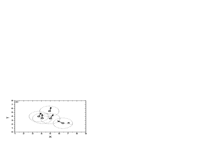
Figure 1: a) Particles interact via short range, local interactions extending over a neighborhood of radius $R$. b) The graph of the weight function (8) where $d=\|\vec{r}_{t}^{i}-\vec{r}_{t}^{j}\|$ denotes the interparticle distance.

The coalescence of coherence and novelty observed in real collectives of motiles suggests to consider an heuristic function $\Phi_{t}^{i}$ being able to display behaviors ranging from order to fully developed chaos. As well known, the logistic map $x_{t+1}=\mu x_{t}(1-x_{t})$ with $x\in[0,1]$ and $0<\mu\leq 4$ [3], is a minimal representative model for the class of discrete dynamical systems unfolding the route to chaos via a period-doubling bifurcation cascade. Hence, we propose the following function

$$\mathbf{\Phi}_{t}^{i}=\Delta_{0}-2\cdot\Delta_{0}\cdot\phi_{t}^{i}\cdot\left(1-\left(\frac{\theta_{t}^{i}}{\Delta_{0}}\right)^{2}\right)$$ (5)

which is obtained by introducing the change of variable

$$x_{t}\rightarrow\frac{1}{2}\left(1-\frac{\theta_{t}}{\Delta_{0}}\right)\mathrm{\;and\;\mu\rightarrow 4\phi}$$ (6)

in the logistic map. Here, the functions $\phi_{t}^{i}\Bigr{(}\left\{\vec{r}_{t}^{j},\vec{v}_{t}^{j}\right\}_{j\neq i}\Bigl{)}$ in (5) should embody the coupling between particles in such a way that conditions a - f are satisfied. As it is shown throughout the forthcoming sections, the latter is achieved by the following function

$$\phi_{t}^{i}=\begin{cases}1-\frac{1}{2sn_{i}}\;\underset{j\in D_{i}(R)}{\sum}\|\vec{v}_{t}^{i}-\vec{v}_{t}^{j}\|w_{i,j}\;&\textrm{if }n_{i}>0\\ 1&\textrm{if }n_{i}=0\end{cases},$$ (7)

where $n_{i}$ is the number of neighboring particles counted within a neighborhood $D_{i}(R)$ of fixed radius $R$ around each particle $i$. Such neighborhood guarantees the validity of condition a. The interaction of neighboring particles $i$ and $j$ is weighted by a suitably chosen function $w_{i,j}$ which aims at satisfying condition b. In particular, we shall assume that $w_{i,j}$ is given by

$$w_{i,j}=\frac{R^{K}}{R^{K}+\left(\|\vec{r}_{t}^{i}-\vec{r}_{t}^{j}\|\right)^{K}}.$$ (8)

Here, the parameter $K$ controls the degree of dependence of the coupling on the interparticle distance. Notice that function (8) approaches a step function as $K$ increases (see Fig. 1(a)). As it turns out, for $K\gg 1$ the effect of different interparticle distances practically disappears, as the contributions of all interparticle couplings, within the neighborhood, tend to be equally weighted.

3 Local Dynamics

We proceed now to the more ‘microscopic’ local level in order to elucidate the underlying dynamics of particle-particle interactions. It is instructive to consider one particle in isolation and subsequently a single pair of particles and their interaction. In a sense this is analogous to the statistical mechanical treatment of ‘dilute gas’ where the particles’ collisions, being rare, are described very accurately by their binary collisions. Since, at very low densities, binary interactions are the most dominant contributions in the present model, we shall consider such a scenario in this section.

3.1 The one particle case

Let us consider first a single particle with its parameter $\phi_{t}^{1}=\phi$ being a constant. In the present case, the whole information about the possible types of particle trajectories is contained in the bifurcation scenario for the variable $\theta_{t}$ as a function of $\phi$. Such bifurcation diagram is qualitatively the same as in the logistic map, as it is carried through by the transformations (6) and $\phi=\mu/4$. As shown in Fig. 2a), the bifurcation diagram of the rotation phase depicts fixed points in the interval $[0,\frac{3}{4}]$, the emergence of multiple period orbits [MPO] in the interval $(\frac{3}{4},F_{p}]$ (where $F_{p}\approx 0.8925$ corresponds to the well-known Feigenbaum accumulation point [3]), onset of chaos at $F_{p}$, coexistence of weak chaos and periodic motion in $(F_{p},1)$ and finally, fully developed chaos at $\phi=1$. It is emphasized here that for $0<\phi<\frac{1}{4}$ the rotation phase attains a maximum value corresponding to the trivial stationary solution $\theta=\Delta_{0}$ of eqs. (4) - (5). For $\frac{1}{4}<\phi<\frac{3}{4}$ the rotation phase is given by $\theta=\frac{1-2\phi}{2\phi}\Delta_{0}$. The particle thereby follows closed trajectories with a radius of curvature growing as $\phi\rightarrow\frac{1}{2}$. At $\phi=\frac{1}{2}$ a change in the sign of the rotation occurs, from anticlockwise for $0\leq\phi<\frac{1}{2}$ to clockwise for $\frac{1}{2}<\phi\leq\frac{3}{4}$. In order to characterize the trajectories of the particles in the interval $[\frac{3}{4},1]$, it is worth considering the mean rotation phase

Figure 2: a) Bifurcation diagram of $\theta_{t}/\Delta_{0}$ as a function of the parameter $\phi$. b) Similar plot for the mean phase $\langle\theta_{t}\rangle/\Delta_{0}$ (see eq. (9)). The inset of panel (b) provides a zoom-in for $\langle\theta_{t}\rangle/\Delta_{0}$ in the $\phi$-interval $(0.89,1]$.

$$\left\langle\theta\right\rangle=\frac{1}{m}\sum_{k=1}^{m}\theta^{(k)}$$ (9)

where m denotes the period of a certain orbit and $\theta^{(k)}$ denotes its $k^{\mbox{\mbox{{th}}}}$ element. In the $\phi$-interval $(\frac{3}{4},0.862]$, which corresponds to orbits of period 2, the mean rotation phase reads $\left\langle\theta\right\rangle=\frac{\Delta_{0}}{4\phi}$. Providing an analytic expression for $\left\langle\theta\right\rangle$ in the case of orbits of period higher than 2 is a cumbersome task and therefore, for $0.862<\phi\leq 1$, we calculate numerically the values of $\left\langle\theta\right\rangle$. These results are presented in panel (b) of Fig. 2. For $\phi$ values in the interval $(0.862,F_{p})$, the trajectories are closed and clockwise. For $\phi$ in the interval $(F_{p},1)$, the mean phase $\left\langle\theta\right\rangle$ displays highly irregular behavior, where the alternation of windows of weak chaos and periodic behavior gives rise to a fine structure profile. In the case of weak chaos, the particle performs a biased chaotic walk leading to quasi-circular trajectories. All along the interval $(F_{P},1)$, the particle motion is clockwise on the average. The peaks observed in Fig. 2(b), where $\left\langle\theta\right\rangle$ attains higher values, are indicative of the presence of windows of periodicity. Finally, at the limiting case of fully developed chaos (i.e. $\phi=1$), the rotation phase takes values distributed within the interval $[-\Delta_{0},\Delta_{0}]$, according to the invariant density

$$\varrho_{s}(\theta,\phi=1)=\frac{1}{\pi\sqrt{\Delta_{0}^{2}-\theta^{2}}}$$

of map (4) - (5). The even character of $\varrho_{s}$ entails that the particle describes a strongly chaotic walk with $\left\langle\theta\right\rangle=0$, as it is confirmed by Fig. 2(b). This way condition c above is satisfied since, according to (7), all isolated individuals evolve with $\phi_{t}^{i}=1$. This analysis has been carried out for a single particle with an arbitrary fixed value of $\phi$. Yet, the same categorization readily applies to the case of many interacting particles, as long as their coupling parameters $\phi_{t}^{i}$ converge towards a quasi-stationary value. The main results obtained from the one particle case are summarized in Table I.

Table 1: Classification of the asymptotic behavior of $\theta$ and of the particle trajectories, for characteristic domains of the parameter $\phi$.

interval: parameter range	asymptotic behavior of $\theta$	type of trajectory
A: $\phi\in[0,\frac{3}{4})$	stationary state	closed, anticlockwise trajectories for $0<\phi<1/2$; straight trajectories at $\phi=1/2$; clockwise, closed trajectories for $1/2<\phi<3/4$
B: $\phi\in[\frac{3}{4},F_{p})$	multiple period orbits	closed, clockwise trajectories
C: $\phi\in[F_{p},1)$	weak chaos	biased chaotic trajectories (quasi-closed, clockwise trajectories)
D: $\phi=1$	fully developed chaos	unbiased chaotic trajectories

3.2 The two particle case: interparticle synchronization

The case of two particles is useful to consider in order to illustrate some of the control features exercised by the coupling function (7) which, in this particular case, is the same for both particles, $\phi_{t}^{(1)}=\phi_{t}^{(2)}\equiv\phi_{t}^{(1,2)}$. Unless stated otherwise, the set of parameters we use throughout the rest of the paper are: $s=1$, $\Delta t=1$, $R=500$, $\Delta_{0}=\frac{1}{40}\pi$ and $K=1$.

First, it is straightforward to show how condition d is satisfied. Figure 3 depicts the plot of the trajectories of two particles initially being out of the interaction zone and approaching each other along the same axis. Under such conditions, when they both enter the interaction zone, the difference of velocities approaches its maximum value $\|\vec{v}_{t}^{(1)}-\vec{v}_{t}^{(2)}\|\approxeq 2s$ and $w_{i,j}=\frac{1}{2}$. Therefore, as soon as both particles start interacting, the parameter $\phi_{t}^{(1,2)}$ drops sharply from unity to $\frac{1}{2}$, as it is shown in Fig. 3(b). According to Fig. 2(a), a value of $\phi_{t}^{(1,2)}<\frac{3}{4}$ entails a single fixed point for both phases $\theta_{t}^{(1)}$ and $\theta_{t}^{(2)}$. As a result, the difference $|\theta_{t}^{(1)}-\theta_{t}^{(2)}|$ will tend to vanish after a brief transient. The latter can be realized by comparing Figs. 3(b,c,d).

Figure 3: a) Trajectories of two particles initially approaching each other frontally. b) Plot of $\phi_{t}^{(1,2)}$ versus time $t$, corresponding to particles of panel a). c) Similar plot for $\theta_{t}^{(1)}/\Delta_{0}$ and $\theta_{t}^{(2)}/\Delta_{0}$. The parameters used are $s=1$, $\Delta t=1$, $R=500$, $\Delta_{0}=\frac{1}{40}\pi$ and $K=1$.

Moreover, since for $\|\vec{r}_{t}^{(1)}-\vec{r}_{t}^{(2)}\|\rightarrow 0$ the weight $w_{(1,2)}\rightarrow 1$, a further decrease in $\phi_{t}^{(1,2)}$ occurs as both particles get closer (see the decrease towards a minimum value in the plot of Fig. 3(b)). As it was discussed in Subsection 3.1, a low value of $\phi_{t}^{(1,2)}<\frac{1}{3}$ leads both phases to reach their maximum value $\Delta_{0}$ (see Figs. 2a) and b)). This fact is demonstrated by the onset of the plateau appearing in Figs. 3(c,d). Once the phases of the particles reach their maximum value, simultaneously with their minimum phase difference, they follow their course away from each other. As it turns out, condition d is satisfied as both particles turn away sharply instead of colliding frontally (see Fig. 3(a)). Eventually, both particles leave the interaction zone and display again fully erratic trajectories.

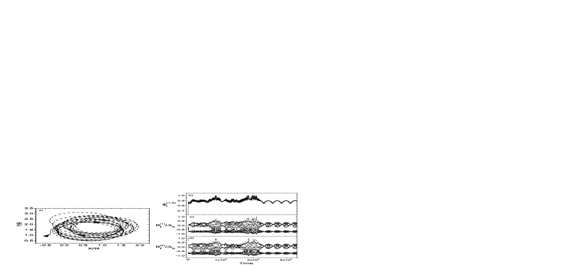
Figure 4: a) Trajectories of two particles located initially inside the interaction zone and approaching each other with a moderate difference of initial velocities. In panel b) we present the plot of $\phi_{t}^{(1,2)}$ versus time $t$ corresponding to particles of panel a). In panels c) and d), we show similar plots for $\theta_{t}^{(1)}/\Delta_{0}$ and $\theta_{t}^{(2)}/\Delta_{0}$ respectively. The parameters we used in these plots are the same as in Fig. 3.

Let us consider now the case of two particles approaching each other inside the interaction zone with a small difference in their initial directions. Figure 4(a) shows the trajectories of two particles in such a typical situation, while Fig. 4(b) depicts the evolution of the coupling parameter $\phi_{t}^{(1,2)}$ and Figs. 4(c,d) show the evolution of the rotation phases $\theta_{t}^{(1)}$ and $\theta_{t}^{(2)}$ of both particles. Initially, a sharp decrease in the difference of directions $\|\vec{v}_{t}^{(1)}-\vec{v}_{t}^{(2)}\|$ occurs, which appears in the plot of Fig. 4(b) as an initial abrupt increase of $\phi_{t}^{(1,2)}$. Since $\phi_{t}^{(1,2)}$ attains a value higher than $\frac{3}{4}$, the rotation phases of both particles subsequently enter into the MPO and chaos regimes. The ongoing evolution process is driven by two counteracting tendencies: The first one is a trend towards strong synchronization if $\phi_{t}^{(1,2)}$ decreases below $F_{P}$. The second one is a trend to spread away if an alignment occurs, i.e. if $\phi_{t}^{(1,2)}\rightarrow 1$. The presence of these two trends is revealed when comparing panels (a), (b) and (c) of Fig. 4: the values of $\theta_{t}^{(1)}$ and $\theta_{t}^{(2)}$ tend to further localize when $\phi_{t}^{(1,2)}$ decreases, while bursts of chaos appear whenever $\phi_{t}^{(1,2)}\approx 1$ (corresponding to an alignment). As it is depicted in Figs. 4(a-c), after a transient self-organization process, the evolution of both particles undergoes a transition towards a highly coherent dynamic regime. The initially irregular behavior observed in the course of the evolution of $\phi_{t}^{(1,2)}$ suddenly disappears and, instead, oscillations emerge within the $\phi$-interval $(0.85,0.9)$. Such oscillations of $\phi_{t}^{(1,2)}$ induce on both phases $\theta_{t}^{(1)}$ and $\theta_{t}^{(2)}$ a regular alternation between windows of high and low period orbits (see Figs. 4 (c,d)). Once such a new regime is attained, both particles tend to move in perfect synchrony and their phase difference $|\theta_{t}^{(1)}-\theta_{t}^{(2)}|$ equals zero, as it is readily shown in Fig. 5. As it turns out, for the case of two particles, it is clear that at longer term the interplay between both tendencies (ordering and chaotic phase spreading) constitute a ‘control mechanism’ that underlies the fulfillment of conditions e and f. Using the set of parameters as in Fig. 3 for different settings of initial conditions, we found that phase synchronization, as it is observed in Fig. 5, occurs provided the initial conditions are such that both particles never leave the interaction zone. In Section 4, we show that phase synchronization is robust in the case of many particles as well.

Figure 5: Corresponding to phases $\theta_{t}^{(1)}$ and $\theta_{t}^{(2)}$ of Fig. 4, the plot of the time evolution of the phase difference $(\theta_{t}^{(1)}-\theta_{t}^{(2)})/\Delta_{0}$.

4 Emergent global dynamics and patterns of motion

Having seen the role of spontaneous synchronization in binary interactions we can now consider the full collective motion problem. As we shall demonstrate further in this section, synchronization is an underlying mechanism for coherent and cohesive motion. Another feature of this intrinsic and coherent steering, which keeps a large fraction of the group together, is that the role of boundary conditions becomes really secondary. Furthermore, we emphasize the fact that the aggregates of motiles keep its coherent motion even in absence of boundaries.

So, let us address now the case of $N$ particles allowed to move on the infinite plane. We consider, thereof, that the initial positions and velocities of the particles are uniformly randomly distributed within a square of side $R_{0}$. Similarly, the rotation phases are distributed in the interval $[-\Delta_{0},\Delta_{0}]$.

In order to capture the spatio-temporal features of the system, such as persistent and/or flickering clustering as well as patterns of cohesion around temporary foci, it is of interest to introduce an index that takes into account both the spatial relations between neighboring particles and the degree of velocity alignments. To this aim, it is instrumental to visualize the system as an undirected graph, where every particle is its node and the edges of the graph are established according to their interparticle distance and to the degree of alignment between particle velocities.

In particular, we consider a pair of nodes as connected if, in addition of being neighbors, the inner angle between their velocities is less than $\Delta_{0}$. Under these assumptions, the time dependent adjacency matrix $\boldsymbol{M}_{t}$ associated to such a graph reads

$$[M_{t}]_{i,j}=\begin{cases}1&\mbox{if }\|\vec{r}_{t}^{(i)}-\vec{r}_{t}^{(j)}\|\leq R\mbox{ and }\|\vec{v}_{t}^{i}-\vec{v}_{t}^{j}\|\leq s\Delta_{0}\\ 0\mbox{ }&\mbox{otherwise}\end{cases}$$ (10)

In terms of this matrix, one can quantify the degree of collective alignment resulting from interparticle interactions by means of the following index

$$\alpha_{t}=\frac{\Gamma_{t}}{\Gamma_{M}},$$ (11)

where $\Gamma_{M}=\tfrac{1}{2}N(N-1)$ is the maximum number of possible connections and $\Gamma_{t}=\frac{1}{2}Tr\left[M_{t}^{2}\right]$ (with $Tr$ denoting the matrix trace and $M_{t}^{2}$ the square of the adjacency matrix) gives the number of actual connections at time $t$. Hereafter we refer to index $\alpha_{t}$ as the Alignment Clustering Index (ACI) at time $t$. Clearly, ACI is an indicator of the degree of coherence of motion of the group of particles. Furthermore, it provides information on the degree of clustering of particles in space and thus it constitutes an indicator of the degree of group cohesion. For instance, strong oscillations in the evolution of the ACI indicate a poorer group cohesion, since its fluctuations reveal that a great amount of particles are merging in as well as escaping from cluster formations.

4.1 Typical patterns and regimes of motion

In order to demonstrate some typical patterns of characteristic behavior of our model, let us consider a collective of particles initially distributed in a squared region of side $R_{0}=\dfrac{1}{3}R$. Unless explicitly mentioned, we shall consider the number of particles $N=300$ and the rest of the parameters to be the same as in Fig. 3.

Figure 6: For a system of $N=300$ particles, in absence of boundaries and initially uniformly randomly settled within a squared region of side $R_{0}=\frac{R}{3}$, plots of the positions and velocities at a) $t=0$, b) $t=2\times 10^{3}$, c) $t=6\times 10^{3}$ and d) $t=1.5\times 10^{4}$. The parameters are the same as in Fig. 3.

Figure 6 shows the plot of the positions and velocities of the set of particles at different times in a single realization. Corresponding to the system of Fig. 6, panel (a) of Fig. 7 shows the evolution of the ACI and panel (b) the evolution of the first and second moments of the coupling functions (7) of all particles. One can distinguish between three qualitatively different stages of collective motion, which can be characterized by means of the ACI behavior:

1. Starting from a disordered state, Fig. 6(a), the system undergoes a strong self-organization process, from $t=0$ up to $t\thickapprox 2\times 10^{3}$. This is characterized by low ACI values (see Fig. 7(a)), and by large oscillations at the level of the coupling functions, Fig 7(b). At the end of this stage the collective motion becomes further organized and the group of particles shapes a circular rotational pattern (see Fig. 6(b)).

2. The second stage, which extends approximately from $t\thickapprox 2\times 10^{3}$ up to $t\thickapprox 1\times 10^{4}$, is mainly characterized by a marked increase of the ACI (see Fig. 7(a)). The coupling functions tend to stabilize around a fixed value, as exhibited by the decrease in the amplitude of oscillations of the mean coupling (see Fig. 7(b)). Along this stage, an increasing number of groups of highly aligned particles are formed (see Fig. 6(c)), thereby fulfilling condition e.

3. At the final stage, the system attains a quasi-stationary regime, at $t\thickapprox 1\times 10^{4}$, along which the ACI stabilizes and the coupling functions remain nearly constant (see Figs. 7(a,b)). In such a regime, the standard deviation of the average also tends to stabilize around a rather low value, thereby indicating an enhancement in the coherence of the behavior of the particles (see Figs. 7(c) and 6(d)). Clearly, group cohesion is evidenced by the fact that high values of the ACI are sustained for times as long as $t=1\times 10^{4}$ and beyond. As it turns out, condition f is also satisfied. It is a remarkable fact that the self-organization process leading to such state of higher coherence drives also the average of the coupling functions towards the region around the Feigenbaum point (which is represented by a dashed line in Fig. 7(b)). In other words, a higher degree of coherence is achieved by a process that exhibits a combination of weak chaos and further ordered behavior. This question will be discussed later in Subsection 4.3, where we shall address the cohesion features of the presented system.

Figure 7: Corresponding to the realization of Fig. 6, the evolution of the ACI is shown in panel a). In panel b), the mean value of the coupling functions $\phi_{t}^{i}$ of all particles (where bars provide the corresponding standard deviation) is presented. The dashed line of panel a) corresponds to the value of the Feigenbaum point.

4.2 Synchronization processes in the collective

In Subsection 3.2 we have shown that the emergence of coherent behavior in the case of two particles arises from synchronization at the level of their rotation phases. Thus, it is natural to inquire on the degree of phase synchronization underlying the coherent aspect of the dynamics of the $N$-particle system as it is exhibited in the plots of Figs. 6 and 7. In order to assess interparticle phase synchronization in a quantitative manner, we shall consider the ensemble of the distinct interparticle phase differences $\Delta\theta_{ij}=\theta_{i}-\theta_{j}$ with $i\neq j$. We shall, thus, monitor the evolution of the system in terms of its synchronized population fraction. Such task is achieved by quantifying the percentage $P_{t}(\Delta\theta)$ of pairs of particles with a given phase difference $\Delta\theta$ at time $t$. Thereby, assessing the synchronization process amounts to follow the evolution of $P_{t}(\Delta\theta)$ on the $\Delta\theta$-interval $[-2\Delta_{0},2\Delta_{0}]$ starting from an initial distribution $P_{0}$. Clearly, full synchronization will be present whenever $P_{0}$ converges asymptotically towards a delta distribution at $\Delta\theta=0$.

Figure 8: Plot of the evolution of two different initial distributions of phase differences for $N=300$ particles. Upper panels: Having all particles the same initial phase $\theta$, distribution of phase differences at (a) $t=0$, (b) $t=2\times 10^{3}$, (c) $t=1\times 10^{4}$, (d) $t=4\times 10^{4}$ and (e) $t=1\times 10^{7}$. Lower panels: for particles with initial phases uniformly randomly distributed, at (f) $t=0$, (g) $t=2\times 10^{3}$, (h) $t=1\times 10^{4}$, (i) $t=4\times 10^{4}$ and (j) $t=1\times 10^{7}$. The parameters used in this figure are the same as in Fig. 3. Such numerical experiments supply ample evidence of the existence of an attracting distribution.

Figure 8 exhibits the plot of the distribution $P_{t}(\Delta\theta)$ at different times (from $t=0$ up to $t=1\times 10^{7}$), starting from two different initial phase distributions: in upper panels (from (a) to (e)), the evolution of an initial delta distribution. In lower panels (from (f) to (j)), similar plots corresponding to an initial distribution obtained by assigning uniformly distributed random values to the initial set of phases $\{\theta_{t}^{i}\}$ (the triangular shape in the initial distribution in Fig. 8(f) follows from the correlations introduced by taking the differences between phases). After a very short transient period, the initial correlations of phases corresponding to both distributions are destroyed and new ones are built as a consequence of the initial strong self-organization process described in Subsection 4.1. As it is shown in the upper and lower panels of Fig. 3, phase synchronization gradually emerges. At $t=1\times 10^{4}$ the percentage of pairs with phase difference $|\Delta\theta|<\Delta_{0}/10$ is $38\%$ for the case of the initial delta distribution (Fig. 8(c)) and $40\%$ for the case of the homogeneous initial distribution (Fig. 8(h)). As the process evolves, the interparticle phase synchronization is further enhanced. For instance, in the case of the delta initial distribution, the percentage of pairs with $|\Delta\theta|<\Delta_{0}/100$ at $t=1\times 10^{7}$ equals $36\%$ (Fig. 8(e)) and it equals $60\%$ for the homogeneous one (Fig. 8(j)). Since similar results are obtained for very different types of initial distributions, one concludes that the synchronization phenomenon observed in Fig. 8 is robust for parameter values as in Fig. 3. However, as it is shown in Subsection 4.3, similar self-organization processes are observed in a wide range of $K$-parameter values.

Regarding the relation between the emergence of synchronization and the gradual formation of clusters of aligned particles in space (see Figs. 6(c,d)), it is interesting to inspect the evolution of the relation between pair synchronization and interparticle distance. Figure 9 depicts the plots of phase difference vs interparticle distances for the particle pairs accounted for in the histograms of panels (f) - (j) of Fig. 8. Initially, all pairs are close to each other, having phase differences randomly distributed in the interval $[-2\Delta_{0},2\Delta_{0}]$ (Fig. 9(a)). At $t=2\times 10^{3}$, particles are further spread away and higher density ‘clouds’ appear within a narrower $\Delta\theta$-interval (Fig. 9(b)). The evolution towards a higher degree of organization leads to cluster formation in both space and phase-difference. As it is displayed in Fig. 9(c), at $t=1\times 10^{4}$ most of the pair particles are distributed in two large clusters. Strong synchronization ($\Delta\theta\approx 0$) occurs between particles within the same cluster, as well as between particles belonging to different clusters. Also, many pairs inside and between clusters exhibit phase differences around specific values which correspond to the secondary peaks in the distribution of Fig. 8(h). For a longer time, i.e. $t=4\times 10^{4}$, the main clusters split into smaller lumps within which particles are further synchronized with each other (Fig. 9(e)). At $t=1\times 10^{7}$, a single compact cluster of fully synchronized pairs ($\Delta\theta=0$) still remains. As it turns out, the presence of strong synchronization at long term entails also a high degree of group cohesion.

In comparison with other models of collective behavior, such as Vicsek’s, one naturally expects the degree of group cohesion to decrease along with the initial density of particles. This question, as well as the dependence of the cohesion on the parameter $K$ in the weight function (8), are addressed in the following Subsection.

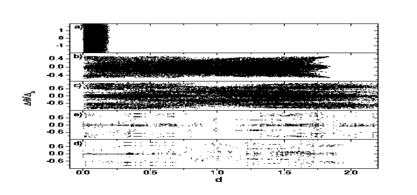
Figure 9: Corresponding to plots f) to j) of Fig. 8, plot of phase differences ($\Delta\theta/\Delta_{0}$) versus interparticle distances at a) $t=0$, b) $t=2\times 10^{3}$, c) $t=1\times 10^{4}$, d) $t=4\times 10^{4}$ and e) $t=1\times 10^{7}$.

4.3 Group cohesion: the role of density and interparticle distances

In the context of animal societies, sharp transitions of collective behavior have been reported to occur at specific values of the population density (see for instance [18, 30, 1, 13, 15, 29, 28, 22]). As it has been already mentioned in the introduction, models belonging to the same class as Vicsek’s exhibit an order-disordered phase transition at a critical value of the particle density. In the model introduced here, the radius of interaction $R$ imposes a characteristic density $\rho^{\star}=N/R^{2}$. Thus, it is natural to study the degree of coherence and cohesion in a group of particles for density values above and below $\rho^{\star}$. Figure 10 depicts the plot of the ensemble average of the ACI for a group of $N=100$ particles at $t=4\times 10^{4}$ and for different values of the ratio $\rho/\rho^{\star}$. This plot exhibits a steep monotonic ascent of the averaged ACI occurring for values $\rho/\rho^{\star}\sim O(10^{-2})$, followed by the onset of a plateau extending for values $\rho/\rho^{\star}>1$. Such a behavior is best fitted by a logistic function of the form

$$\left\langle\alpha(\rho/\rho^{*})\right\rangle_{t=4\times 10^{4}}=a+\cfrac{b}{c^{p}+(\rho/\rho^{*})^{p}}$$ (12)

where $a=0.170$, $b_{0}=0.003$, $c=0.173$ , $b=(b_{0}-a)c^{p}$ and $p=2.460$ (as it is represented in Fig. 10 by a continuous gray line) with a correlation coefficient of about $0.976$.

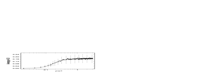
Figure 10: Plot of the ensemble average of the ACI, $\left\langle\alpha_{t}(\rho/\rho^{*})\right\rangle$, of $N=100$ particles at time $t=4\times 10^{4}$ (dots) for different values of the logarithm of the ratio $\rho/\rho^{\star}$. Here the average was taken over an ensemble of $200$ uniformly random initial conditions. The rest of the parameters are the same as in Fig. 3. Bars in the plot indicate the standard deviation. The curve described by these points is best fitted by a logistic function in the form of Eq. (12).

It must be noted here that the choice of the logarithmic scale for the ratio $\rho/\rho^{\star}$ serves in elucidating the abrupt change observed. The change of behavior exhibited in Fig. 10, as described by the logistic form of Eq. (12), differs in nature from the phase transition reported for Vicsek’s class of models [29, 32]. In addition, we stress the fact that the abrupt change in the degree of coherence shown in Fig. 10 arises naturally from the interparticle interactions, through concerted self-adaptation in the steering parameters of the particles.

Figure 11: For a group of $N=100$ particles, plot of the ensemble average of the ACI, at $t=4\times 10^{4}$ for different values of the parameter $K$. Similarly as in Fig. 10, the average is computed over an ensemble of 200 uniformly randomly distributed initial conditions where error bars indicate one standard deviation.

On the other hand, the cohesion of the group is controlled additionally by the parameter $K$ in the weight function (8). Figure 11 shows the plot of the ensemble average of the ACI at $t=4\times 10^{4}$ for different values of $K$. One observes that stronger cohesion, as gauged by the ACI, is attained for small values of $K$. For $0<K\leq 1.25$, the average ACI takes values around $15-20\%$. A decrease in the averaged ACI is observed in the interval $0<K\lesssim 5$ which is followed by an increase for $5<K\lesssim 10$. For $K$ values greater than 10, the averaged ACI gradually decreases. It is noticeable that the change in the overall behavior of the ACI around $K=5$, from decrease to increase, coincides with the change of sign in the curvature of the graph of weight functions $W_{{i},{j}}$ of (8) when varying $K$. Since the form of the weight functions ultimately affects the behavior of the coupling functions $\phi_{i}$ of (7), it is worth considering the ensemble average of the histograms of the coupling functions of all particles. In particular, we shall focus on the main regions described in Table I, namely A: a steady state, B: multi-periodicity, C: weak chaos and D: fully developed chaos.

Figure 12 displays the ensemble average of the histograms obtained at different times and for different values of $K$. Initially (first column of Fig. 12), regardless of the value of $K$, one observes that the coupling functions take values in the region where a steady state exists. For $K=1$ (first row of Fig. 12), the values of the couplings gradually evolve towards the region of multi-periodicity and beyond. At $t=4\times 10^{4}$ one observes that the bulk of particles is equally distributed between the multi-periodicity and weak chaos regions. However, $10\%$ of the particles also appear in the region of fully developed chaos, which reveals particle escapes away from the center of mass. In the cases $K=5$, $K=10$ and $K=15$ (rows 3, 4 of Fig. 12), at long times, more than $20\%$ of the particles have escaped and those that remain confined exhibit $\phi_{i}$-values mostly in the regions corresponding to stationarity and multi-periodicity. Summarizing, in the case $K=1$, a higher degree of coherence and group cohesion is attained through a process encompassing balance between weak chaos and ordered behavior. In the cases $K=5$, $K=10$ and $K=15$, where most of the interacting particles display further ordered behavior, the degree of cohesion is poorer. In particular, in the case $K=5$ almost $40\%$ of the particles have escaped at $t=4\times 10^{4}$ (as it is indicated by an increased number of particles with $\phi_{j}\in D$). Consequently, for $K=5$, the averaged ACI attains a very low value of approximately 0.05 (see Fig. 11). For $5<K<10$, a further rigid steering motion arises, as an increased number of particles having $\phi_{j}\in\mbox{A}$ tend to display short concentric trajectories. Thereby, the number of escapes is smaller and the average ACI becomes higher than in the case of $K=5$ (see Fig. 11). The latter provides an insight into the origin of the minimum of the averaged ACI observed around $K=5$.

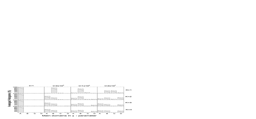
Figure 12: Plots of the ensemble average of histograms obtained from a group of $N=100$ particles for the $\phi$-intervals of Table I which correspond to A: a steady state, B: multi-periodicity, C: weak chaos and D: fully developed chaos (the percentage of particles in D indicates the proportion of isolated particles). The average was taken over an ensemble of 200 initial conditions. Columns from left to right in this plot present results obtained for $t=1$, $t=2\times 10^{3}$, $t=1\times 10^{4}$ and $t=2\times 10^{4}$ while rows from top to bottom correspond to results obtained for $K=1$, $K=5$, $K=10$ and $K=15$. The rest of the parameters are the same as in Fig. 3.

5 Conclusions

In this work we have introduced a minimal model of motile particles which takes into account an intrinsic steering mechanism. Its main feature is that it exhibits the emergence of patterns of coherent collective motion. Since each particle is endowed with an intrinsic mechanism, it allows it to adjust its trajectory according to the surrounding conditions. With this extra feature the model can be of utility as an augmented inert particle model. The adaptation is achieved by changes which are determined by a map of the logistic-map family, which displays fully developed chaos in absence of interparticle interactions. As it turns out, isolated particles behave as chaotic walkers. On the other hand, particles within a neighborhood of fixed radius interact with each other by establishing nonlinear couplings between their corresponding logistic maps. The coupling between a particle and its surrounding neighbors is embodied by a function that depends explicitly on the positions and velocities of the set of involved particles. The coupling functions play their role in self-adapting the controlling parameters of the logistic map at the individual level of each motile by ‘tuning in’ the behavior of each particle. This behaviour can range from single to multiple periodic and chaotic regimes. The explicit form of the coupling functions is such that frontal collisions are hindered and that neighboring particles undergo a self-organization process leading to the emergence of coherent collective motion. The whole process is characterized by an index, called ACI (and denoted by $\alpha$ herein). This graph index, captures the essential features of the system’s time evolution, since it quantifies the degree of cohesion and alignment of particles. It is shown that the self-organization process of steering leads the collective of these motiles towards a regime of coherence and group cohesion. The latter is shown to be essentially related to the phase synchronization that emerges between the inner steering mechanisms of the particles.

Also, the degree of group coherence is studied as a function of a parameter $K$. This parameter sets the dependence of the interactions on the interparticle distances. Such a study shows that higher levels of coherence and group cohesion occur in cases where most of the particles exhibit a balanced combination of ordered motion (multi-periodicity) and weakly chaotic behavior.

Similarly, as in other reported cases, the system presented here exhibits a drastic change in the degree of coherence as a function of the initial particle density but in a more abrupt fashion. However, such result does not require the use of periodic boundary conditions as it is customary the case in other classes of models.

Further investigation of this model is required in order to develop insights on key questions regarding the phenomenon of phase synchronization observed, as well as, the dependence of the characteristic time of synchronization on the model parameters and on how robustness of synchronization is affected by the density of particles.

On the other hand, since our system can be considered of the minimal ones that includes a deterministic steering, it can be readily augmented in order to account for more realistic situations. Depending on the context of application one might easily consider further the inclusion of particle accelerations, different types of long or short range interactions for the interparticle attraction, inclusion of inhomogeneities and ambient gradients effectuated at the level of the interactions and finally the introduction of population variability such as groups of leading and/or inert particles.

References

- [1] S. Camazine, J. L. Deneubourg, N. R. Franks, Self - Organization in Biological Systems, Princeton University Press, 2003.
- [2] G. Nicolis, C. Nicolis, Foundations of Complex Systems, World Scientific, 2007.
- [3] G. Nicolis, Introduction to Nonliner Science, Cambridge University Press, 1999.
- [4] I. Giardina, Collective behavior in animal groups: Theoretical models and empirical studies, HFSP Journal 2 (4) (2008) 205–219.
- [5] T. Feder, Statistical physics is for the birds, Physics Today (2007) 28–30.
- [6] J. K. L. Edelstein, K. Parrish, Complexity, pattern, and evolutionary trade - offs in animal aggregation, Science 284 (1999) 99.
- [7] K. Kaneko, Relevance of dynamic clustering to biological networks, Physica D 75 (1994) 55–73.
- [8] A. Chowdhury, D. Schadschneider, K. Nishinari, Physics of transport and traffic phenomena in biology: From molecular motors and cells to organisms, Physics of Life Reviews 2 (2005) 318–352.
- [9] C. Mateo, What the flock is: Emergent collective motion, Physics 569: Emergent States of Matter, Fall 2009, at the University of Illinois at Urbana - Champaig (19 Dec. 2008).
- [10] S. V. Parrish, J. K. Viscido, D. Grunbaum, Self - organized fish schools: An examination of emergent properties, Biol. Bull. 202 (2002) 296–305.
- [11] A. Ackland, G. Wood, Evolving the selfish herd: Emergence of distinct aggregating strategies in an individual - based model, Proceedings of the Royal Society B: Biological Sciences 274 (2007) 1637–1642.
- [12] J. Kolpas, A. Moehlis, I. G. Kevrekidis, Coarse - grained analysis of stochasticity - induced switching between collective motion states, Proceedings of the National Academy of Sciences of the United States of America 104 (14) (2007) 5931–5935.
- [13] F. J. Dossetti, V. Sevilla, V. M. Kenkre, Phase transitions induced by complex nonlinear noise in a system of self - propelled agents, Phys. Rev. E 79 (2009) 051115.
- [14] M. M. Rauch, E. M. Millonas, D. R. Chialvo, Pattern formation and functionality in swarm models, Phys. Lett. A 207 (1995) 185–193.
- [15] G. Grégoire, H. Chaté, Onset of collective and cohesive motion, Physical Review Letters 92 (2) (2004) 025702–1.
- [16] M. Cosenza, M. G. Pineda, A. Parravano, Emergence patterns in driven and in autonomous spatiotemporal systems, Phys. Rev. E 67 (2003) 066217.
- [17] L. M. Parravano, A. Reyes, Gaslike model of social motility, Phys. Rev. E 78 (2008) 026120.
- [18] W. Schweitzer, F. Ebeling, B. Tilch, Statistical mechanics of canonical - dissipative systems and applications to swarm dynamics, Phys. Rev. E 64 (2001) 021110.
- [19] T. Kaneko, K. Shibata, Coupled map gas: structure formation and dynamics of interacting motile elements with internal dynamics, Physica D 181 (2003) 197–214.
- [20] W. Erdmann, U. Ebeling, V. S. Anishchenko, Excitation of rotational modes in two - dimensional systems of driven Brownian particles, Phys. Rev. E 65 (2002) 061106.
- [21] D. Kulinskii, V. L. Ratushnaya, V. I. Bedeaux, A. V. Zvelindovsky, Collective behavior of self - propelling particles with kinematic constraints: The relation between the discrete and the continuous description, Physica A 381 (2007) 39–46.
- [22] H. T. Chen, M. Z. Li, W. Zhang, T. Zhou, Singularities and symmetry breaking in swarms, Phys. Rev. E 77 (2008) 021920.
- [23] J. L. Deneubourg, S. Goss, Collective patterns and decision - making, Ethology, Ecology and Evolution 1 (1989) 295–311.
- [24] K. Kaneko, Pattern dynamics in spatiotemporal chaos, Physica D 34 (1987) 1–41.
- [25] O. Miramontes, Order - disorder transitions in the behavior of ant societies, Complexity 1 (3) (1995) 56–60.
- [26] F. Smale, S. Cucker, Emergent behavior in flocks, IEEE Transactions on Automatic Control 52 (5).
- [27] F. Smale, S. Cucker, On the mathematics of emergence, Japanese Journal of Mathematics 2 (1) (2007) 197–227.
- [28] O. J. Evans, M. R. O’Loan, Alternating steady state in one - dimensional flocking, J. Phys. A: Math. Gen. 32 (1999) L99–L105.
- [29] I. Nagy, M. Daruka, T. Vicsek, New aspects of the continuous phase transition in the scalar noise model (SNM) of collective motion, Physica A 373 (2007) 445–454.
- [30] M. Aldana, V. Dossetti, C. Huepe, Phase transitions in systems of self - propelled agents and related network models, Phys. Rev. Lett. 98 (2007) 095702.
- [31] R. Charrier, L’intelligence en essaim sous l’angle des systemes complexes, Ph.D. thesis, Universite Nancy II (27 Nov. 2009).
- [32] F. Grégoire, G. Peruani, F. Chaté, H. Ginelli, F. Raynaud, Modeling collective motion: Variations on the Vicsek model, European Physical Journal B 64 (3 - 4) (2008) 451–456.
- [33] I. Bonzani, Hydrodynamic models of traffic flow: Drivers’ behaviour and nonlinear diffusion, Mathematical and Computer Modelling 31 (6 - 7) (2000) 1–8.
- [34] M. R. Avila, Synchronization phenomena in light-controlled oscillators, Ph.D. thesis, Université Libre de Bruxelles, Service de Chimie Physique (2004).
- [35] S. Sarkar, P. Parmananda, Synchronization of an ensemble of oscillators regulated by their spatial movement, Chaos 20 (4) (2010) 043108–1–043108–8.
- [36] L. L. Zonia, B. D., Swimming patterns and dynamics of simulated Escherichia coli bacteria, J. R. Soc. Interface 6 (2009) 1035–1046.
- [37] M. Samaey, G. Rousset, Individual-based models for bacterial chemotaxis and variance reduced simulations, Research Report INRIA-00425065, INRIA, Université des Sciences et Technologies de Lille - Lille I (2009).
- [38] A. F. T. Winfield, Encyclopedia of Complexity and System Science, Springer, 2009, Ch. Foraging Robots, pp. 3682–3700.