Noise Can Reduce Disorder in Chaotic Dynamics

Abstract

We evoke the idea of representation of the chaotic attractor by the set of unstable periodic orbits and disclose a novel noise-induced ordering phenomenon. For long unstable periodic orbits forming the strange attractor the weights (or natural measure) is generally highly inhomogeneous over the set, either diminishing or enhancing the contribution of these orbits into system dynamics. We show analytically and numerically a weak noise to reduce this inhomogeneity and, additionally to obvious perturbing impact, make a regularizing influence on the chaotic dynamics. This universal effect is rooted into the nature of deterministic chaos.

1 Introduction

During few recent decades, noise was found to have ability not only to make an obvious disordering impact, but also to play a constructive role, increasing degree of order in system dynamics McNamara-Wiesenfeld-1989 ; Gammaitoni-etal-1998 ; Pikovsky-Kurths-1997 ; Anishchenko-1995 ; Zhou_etal-2002 ; Teramae-Tanaka-2004 ; Goldobin-Pikovsky-2005a ; Goldobin-Pikovsky-2005b ; Goldobin-etal-2010 ; Anderson-1958 ; Maynard-2001 ; Goldobin-Shklyaeva-2009 ; Goldobin-Shklyaeva-2013 ; Altmann-Endler-2010 . Most remarkable advances are the phenomena of stochastic McNamara-Wiesenfeld-1989 ; Gammaitoni-etal-1998 and coherence resonances Pikovsky-Kurths-1997 ; the suppression of deterministic chaos in dynamics of dissipative systems by noise (thoroughly discussed, e.g., in Anishchenko-1995 ); noise-induced enhancement of the phase synchronization of chaotic systems Zhou_etal-2002 ; synchronization by common noise Teramae-Tanaka-2004 ; Goldobin-Pikovsky-2005a ; Goldobin-Pikovsky-2005b ; Goldobin-etal-2010 ; Anderson localization Anderson-1958 ; Maynard-2001 ; the analog of the latter phenomenon for dissipative systems Goldobin-Shklyaeva-2009 ; Goldobin-Shklyaeva-2013 ; etc. In this paper we disclose a novel phenomenon, where weak noise reduces disorder in chaotic dynamics. The effect is rooted in inhomogeneity of the distribution of natural measure over the strange attractor and impact of noise on this distribution.

First, we demonstrate this inhomogeneity and reason for the consequences expected from it. Then we construct an analytical theory for the noise impact. Finally, the predictions of the analytical theory are underpinned with results of simulation for paradigmatic chaotic system, the Lorenz one Lorenz-1963 , where one can see the disorder reduction effect with divers quantifiers of regularity, and for the mapping which is relevant for one of the classical routes of the transition from regular dynamics to chaotic one Lyubimov-Zaks-1983 .

In our treatment we relay on the idea of representation of chaotic attractor by the set of UPOs embedded into it (Grebogi-Ott-Yorke-1988 ; Ott_book , etc.). On this way, for instance, one can evaluate the average $\overline{A}$ for the chaotic regime as $\overline{A}=\int A({\bf x})\mu({\bf x})d{\bf x}$, where $\mu$ is the natural measure, and integration is performed over the whole attractor. It was shown in Grebogi-Ott-Yorke-1988 (see also the text book Ott_book ) that the distribution of natural measure over attractor can be recovered from properties of the UPOs. For two-dimensional maps (and therefore three-dimensional dynamic systems where one can use Poincaré section to construct such a map) the natural measure of an UPO is $\mu\propto\Lambda^{-1}$ where $\Lambda$ is the largest multiplier of perturbations of this UPO. This result is treated to be valid in higher dimensions as long as we have only one positive Lyapunov exponent Grebogi-Ott-Yorke-1988 . The approach was employed already in Eckhardt-Ott-1994 for evaluation of fractal characteristics of the Lorenz attractor from the UPOs data weighted with measure $\mu\propto\Lambda^{-1}$.

The effect under consideration may shed light on fine mechanisms (or one of them) of phenomena similar to the noise-induced enhancement of the phase synchronization of chaotic systems Zhou_etal-2002 .

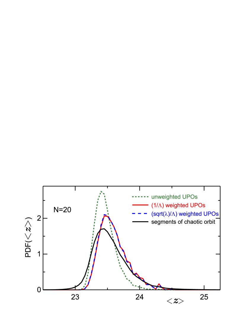
Figure 1: Probability density function of $\langle{z}\rangle$ calculated for the Lorenz system with classical set of parameters ($\sigma=10$, $b=8/3$, $r=28$) over UPOs of length $N=20$ without weight (doted green line); with weight $\Lambda^{-1}$ (solid red line), which corresponds to UPO’s measure within chaotic attractor in noise-free case; with weight $\sqrt{\lambda}/\Lambda$ (dashed blue line), which corresponds to the maximal correction of the weight induced by a weak noise; and $20$-loop segments of chaotic orbit (solid black line).

2 Inhomogeneity of natural measure distribution

We consider the Lorenz system Lorenz-1963 , as an example,

$$\frac{dx}{dt}=\sigma(y-x),\quad\frac{dy}{dt}=rx-y-xz,\quad\frac{dz}{dt}=xy-bz.$$ (1)

Recently Zaks-Goldobin-2010 , we reported the results of calculation of all UPOs with length $N\leq 20$ (by “lenght” of UPO we mean the number of loops). In Fig.1 one can see probability density function (PDF) of $\langle{z}\rangle$ calculated over UPOs of length $N=20$, the distribution weighted with $\Lambda^{-1}$ and PDF of $\langle{z}\rangle$ calculated over $20$-loop segments of the chaotic trajectory. The unweighted and weighted distributions are remarkably dissimilar and the latter matches the chaotic averaging much better. The weighted distribution possesses a relatively big tail for large $\langle{z}\rangle$, where there is a quite few number of UPOs (unweighted PDF nearly riches zero next to $\langle{z}\rangle=24$). The origin of this difference is a huge dispersion of multipliers for long UPOs: for $N=20$ the smallest multiplier $\Lambda=62\,200$ is by factor $72.8$ smaller than the largest one $\Lambda=4\,527\,160$. Noteworthy, the weighted distribution is significantly broader than the unweighted one. This feature implies a large contribution of relatively small number of UPOs with extreme deviation of properties from the typical ones (e.g., in Fig. 1 these UPOs have untypically large values of $\langle{z}\rangle$). In terms of temporal evolution, the system dynamics is strongly inhomogeneous: the epoches of “typical” behaviour intermit with the epoches spent near several least unstable “untypical” periodic orbits.

Such a huge inhomogeneity of multipliers evokes the questions: (i) How this inhomogeneity is effected by weak noise? (ii) What are the consequences for the system dynamics? Indeed, the set of UPOs is dense and even infinitely small perturbation throws the system from one UPO onto another. Hence, one can expect that a very weak noise could first influence the rules of walking over this set and only then affect properties of UPOs. One can expect (and the aim of this paper is to validate relevance of such expectations) the noise to play a “smoothing” role, reducing inhomogeneity of multipliers. As a result of such smoothing, one should observe, in particular, shrinking of the distribution of $\langle{z}\rangle$ calculated over finite segments of the chaotic trajectory because unweighted distribution is more narrow than the weighted one.

3 Effect of noise on natural measure distribution

A significant advance in analytical description of noise action on systems with fine structure was made for one-dimensional maps Cvitanovic_etal-1998 ; Dettmann-Howard-2009 ; Lippolis-Cvitanovic-2010 . In Cvitanovic_etal-1998 the formalism of Feynman diagrams was employed for treatment of noisy dynamics as a perturbation to deterministic dynamics over the set of periodic orbits. In Dettmann-Howard-2009 the escape rates for unimodal maps were evaluated. However, in higher dimensions—which are practically inevitable when the map is a Poincaré map of chaotic continuous-time dynamic system—analytical advance becomes restricted; studies require ad hoc approaches and/or more numerics Gaspard-2002 ; Altmann-Endler-2010 ; Altmann-Leitao-Lopes-2012 . Studies Cvitanovic_etal-1998 ; Dettmann-Howard-2009 ; Lippolis-Cvitanovic-2010 ; Gaspard-2002 ; Altmann-Leitao-Lopes-2012 formed solid instrumental and theoretical basis for working with the noise-induced effects in the systems with fine structure.

Nonetheless, in our study we do not employ the advanced zeta function formalism and use its limiting version assessing the measure merely with leading multipliers Cvitanovic_etal-chaosbook . This version well proved itself for practical applications Grebogi-Ott-Yorke-1988 ; Eckhardt-Ott-1994 and is easier from the view point of calculations when one need as many UPOs as all the UPOs with $\leq 20$ loops. Noteworthy, for most problems addressed in literature, low-length periodic orbits provide enough data for an accurate description Cvitanovic_etal-1998 ; Dettmann-Howard-2009 , whereas in our case inhomogeneity of high-length orbits is essential. Another reason to use simplified (though still accurate) formalism of Grebogi-Ott-Yorke-1988 is that the analytical theory we will construct is rather qualitative and is purposed to highlight the mechanism of the effect which will be finally demonstrated with results of the direct numerical simulation for chaotic systems.

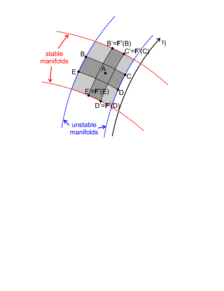
Figure 2: Cell on the Poincaré surface limited by stable and unstable manifolds of the chaotic attractor in the vicinity of fixed point $\mathrm{A}$. In the vicinity of fixed point $\mathrm{A}$ of map ${\bf F}^{k}$, curvilinear parallelogram $\mathrm{B^{\prime}C^{\prime}D^{\prime}E^{\prime}}$ is the image of $\mathrm{BCDE}$.

For evaluation of natural measure, we first briefly recall its calculation for the no-noise case (interested readers can find a detailed rigorous consideration in Sec. VI of Grebogi-Ott-Yorke-1988 ). We consider certain Poincaré section and two-dimensional map on it, which is induced by three-dimensional phase flow. We are interested in calculation of the natural measure distribution over attractor on the Poincaré surface. Let us consider $k$ iterations of the map, ${\bf x}_{n+k}={\bf F}^{k}({\bf x}_{n})$, where $k$ is large, and a small cell bounded by stable and unstable manifolds, which feature the directions of compaction and stretching of the phase volume, respectively, as sketched in Fig. 2. In the vicinity of fixed point $\mathrm{A}$ of map ${\bf F}^{k}$, curvilinear parallelogram $\mathrm{B^{\prime}C^{\prime}D^{\prime}E^{\prime}}$ is formed by states belonging the cell before $k$ iterations of the map, and $\mathrm{BCDE}$ is the pre-image of this parallelogram. By definition of the ergodic (mixing) attractor, for any two subsets $S_{a}$ and $S_{b}$ in the phase space of the system, we have

$$\lim_{k\to\infty}\mu[S_{a}\bigcap{\bf F}^{k}(S_{b})]=\mu(S_{a})\,\mu(S_{b}).$$

If we take $S_{a}$ and $S_{b}$ to be the cell we consider, then $\mu(\mbox{cell})=\mu(\mathrm{BCDE})/\mu(\mbox{cell})=\mu(\mathrm{B^{\prime}C^{\prime}D^{\prime}E^{\prime}})/\mu(\mbox{cell})$. Furthermore, the measure varies smoothly along the unstable direction Bowen-1978 (this is quite general in nature, that the stretching/expansion is a smoothing process), while it typically has a complex inhomogeneous structure in the stable direction, which is transversal to the chaotic attractor. Therefore, one can easily compare the measure of the cell and parallelogram $\mathrm{BCDE}$: their ratio is the ratio of their extension along the unstable direction, because these two sets have one and the same structure and extension along the “complex” inhomogeneous stable direction. We find $\mu(\mbox{cell})=\mu(\mathrm{BCDE})/\mu(\mbox{cell})=\mathrm{CD}/\mathrm{C^{\prime}D^{\prime}}=1/\Lambda_{{\bf F}^{k}}(\mathrm{A})$, where $\Lambda_{{\bf F}^{k}}(\mathrm{A})$ is the largest eigen value of fixed point $\mathrm{A}$ of map ${\bf F}^{k}$. Recall, that we have found the measure associated with a single fixed point $\mathrm{A}$; when there is more fixed points in the cell one has to sum contributions of all of them,

$$\mu(\mbox{cell})=\lim_{k\to\infty}\sum_{\mbox{fixed points in cell}}\frac{1}{\Lambda_{{\bf F}^{k}}(\mathrm{A}_{j})}.$$

Henceforth, the subscript $j$ indicates the number of a fixed point or the corresponding UPO. This result was derived in Grebogi-Ott-Yorke-1988 . Recall, the presented evaluation implies that attractor is hyperbolic, i.e., the stable and unstable manifolds are not mutually tangent anywhere. Although the Lorenz attractor is non-hyperbolic, it is generally accepted that statistically significant measure distribution is determined by the same law $1/\Lambda$.

This calculation of the natural measure sheds light on the fact that we have to track only the coordinate along the unstable manifolds, say $\eta$, and evaluate the fraction of states in the $\varepsilon$-vicinity of some UPO, for which $\eta$ stays within the $\varepsilon$-vicinity. In no-noise case, the fraction of such states is simply $1/\Lambda$. Now let us evaluate such a fraction in the presence of a weak Gaussian $\delta$-correlated noise $a\xi(t)$: $\langle\xi(t)\rangle=0$, $\langle\xi(t)\xi(t^{\prime})\rangle=2\delta(t-t^{\prime})$, $a$ is the noise amplitude.

Our map is induced by a continuous time evolution and in the presence of time-dependent signal, noise, one has to deal with a continuous-time evolution. Placing the origin of the $\eta$-axis at fixed point $A_{j}$, one can find

$$\eta(t_{0}+T_{j})=\Lambda_{j}\eta(t_{0})+a\int\limits_{0}^{T_{j}}f[{\bf x}_{j}(\tau)]\,\xi(t_{0}+\tau)\,e^{\lambda_{j}(T_{j}-\tau)}d\tau=\Lambda_{j}\eta(t_{0})+\alpha R\,,$$ (2)

where $T_{j}$ is the period of UPO ${\bf x}_{j}(t)$ associated with $A_{j}$, $f({\bf x})$ is the susceptibility to noise, $\lambda_{j}=T_{j}^{-1}\ln\Lambda_{j}$ is the leading Lyapunov exponent of the $j$-th UPO, $R$ is the Gaussian random value of unit variance, $\langle{R^{2}}\rangle=1$, and

$$\alpha^{2} \equiv a^{2}\left\langle\left(\int\limits_{0}^{T_{j}}f[{\bf x}_{j}(\tau)]\,\xi(t_{0}+\tau)\,e^{\lambda_{j}(T_{j}-\tau)}d\tau\right)^{2}\right\rangle$$

$$= 2a^{2}\int\limits_{0}^{T_{j}}f^{2}[{\bf x}_{j}(\tau)]\,e^{2\lambda_{j}(T_{j}-\tau)}d\tau=\frac{a^{2}F_{j}^{2}(\Lambda_{j}^{2}-1)}{\lambda_{j}}\,.$$

Here $F_{j}$ is the characteristic value of $f[{\bf x}_{j}(\tau)]$;

$$F_{j}^{2}\equiv 2\lambda_{j}\,(1-\Lambda_{j}^{-2})^{-1}\int\limits_{0}^{T_{j}}f^{2}[{\bf x}_{j}(\tau)]\exp(-2\lambda_{j}\tau)d\tau\,.$$

According to Eq. (2), the probability of $\eta(t_{0}+T_{j})$ to be at the $\varepsilon_{j}$-vicinity of fixed point $A_{j}$ is

$$P(|\eta(t_{0}+T_{j})|\leq\varepsilon_{j}\,|\,\eta(t_{0})) = \int\limits_{\frac{-\varepsilon_{j}-\Lambda_{j}\eta(t_{0})}{\alpha}}^{\frac{\varepsilon_{j}-\Lambda_{j}\eta(t_{0})}{\alpha}}\frac{\displaystyle e^{-\frac{R^{2}}{2}}}{\sqrt{2\pi}}dR$$

$$= \frac{1}{2}\left[\Phi\left(\frac{\varepsilon_{j}-\Lambda_{j}\eta(t_{0})}{\alpha\sqrt{2}}\right)-\Phi\left(\frac{-\varepsilon_{j}-\Lambda_{j}\eta(t_{0})}{\alpha\sqrt{2}}\right)\right],$$

where $\Phi(...)$ is the error function. Finally, the measure of the $\varepsilon_{j}$-vicinity of fixed point $A_{j}$, say $\Omega_{\varepsilon_{j}}(A_{j})$, is

$$\mu[\Omega_{\varepsilon_{j}}(A_{j})] = \int\limits_{-\varepsilon_{j}}^{\varepsilon_{j}}P(|\eta(t_{0}+T_{j})|\leq\varepsilon_{j}\,|\,\eta(t_{0}))\,d(\eta(t_{0}))$$ (3)

$$\approx \frac{1}{\Lambda_{j}}\Phi\left(\frac{\varepsilon_{j}}{F_{j}a}\sqrt{\frac{\lambda_{j}}{2}}\right).$$

The last approximate expression corresponds to the limit of large $\Lambda_{j}$, which is relevant for long UPOs we consider. For vanishing noise, $a=0$, the error function turns $1$, and we have the conventional result of Grebogi-Ott-Yorke-1988 .

One can see in Eq. (3), that for larger $\Lambda_{j}$ (hence, larger $\lambda_{j}$) the argument of $\Phi$ is typically larger. Indeed, although $T_{j}$ also effects the relation between $\Lambda_{j}$ and $\lambda_{j}$, one can find examples of both larger and smaller $T_{j}$ for given value of $\lambda_{j}$. Neglecting correlation between $T_{j}$ and $\lambda_{j}$, one will typically observe the noticed correlation between $\Lambda_{j}$ and $\lambda_{j}$. This correlation decreases inequivalence between UPOs with different weight. Maximal decrease of inequivalence is achieved when the argument of $\Phi$ is small, $(\varepsilon_{j}/F_{j})\sqrt{\lambda/2}\ll a$ ; at this case one finds $\mu\propto\sqrt{\lambda_{j}}/\Lambda_{j}$. In particular, for the $20$-loop UPOs in the Lorenz system the maximal ratio of weights decreases by 15%. In Fig. 1 the distribution of $\langle{z}\rangle$ with weight $\sqrt{\lambda}/\Lambda$ is slightly shrunk compared to the one with $\Lambda^{-1}$.

Notice, the vicinity extension $\varepsilon$ is not precisely known value in our analytical theory. The properties of neighboring UPOs could be similar and, additionally, the measure smoothly varies along the unstable direction on the attractor. Hence, $\varepsilon$ could be not only the characteristic distance between nearest UPOs of length $N$ but rather a considerably larger number featuring the size of clusters of UPOs.

Figure 3: Theoretical dependence of the variance of $\langle{z}\rangle$ for UPOs of length $N=20$ on noise amplitude $a$ for the Lorenz system with classical set of parameters and various values of parameter $\varepsilon$ which measures characteristic vicinity of UPOs. For the sake of demonstration we plot the first term of the expression for the variance [Eq. (4)] (solid lines) which features purely noise-induced redistribution of measure over UPOs of the noise-free system; the dashed lines with symbols represent the total variance with account for the noise-induced dispersion of each single UPO.

4 Effect of noise on disorder quantifiers

Now we calculate the variance of $\langle{z}\rangle$ for UPOs of length $N$ in the presence of weak noise $a\xi(t)$:

$$\mathrm{var}(\langle{z}\rangle_{j})=\sum_{j}\mu_{j}\big{[}\langle{z}\rangle_{j}^{2}-\overline{\langle{z}\rangle}^{2}\big{]}+Ka^{2},\quad\overline{\langle{z}\rangle}=\sum_{j}\mu_{j}\langle{z}\rangle_{j}.$$ (4)

Here we sum the variance related to the distribution over the set of UPOs of the noise-free system and the noise-induced distortion of these UPOs themselves, which is nearly statistically independent from the former and described by term $Ka^{2}$. The value of parameter $K$ is approximately inferred from numerical calculation of the variance of $\langle{z}\rangle$ for the segments of the chaotic trajectory (rough analytical estimation yields the value of the same order of magnitude).

In Fig. 3, we plot the variance of $\langle{z}\rangle$ for UPOs of length $N=20$ for the Lorenz system (1) with the classical set of parameters. We approximately assume $\varepsilon_{j}/F_{j}$ to be the same for all UPOs (notice, $F_{j}$ is of order of $1$). One can note the always-present ordering role of noise which decreases inequality of weights of UPOs: solid lines show decrease of the variance by $2.5\%$. However, this ordering effect can be overwhelmed by the dispersive action of noise on the orbits when $\varepsilon$ is not small enough. For the classical set of parameters the effect is not enough well pronounced and practically unobservable with dispersion of $\langle{z}\rangle$ for chaotic segments. Still, we report the results for this case, where the effect is small, for to emphasize their universality: the effect is always present in some form. For a stronger inhomogeneity of the attractor one can expect a more pronounced effect.

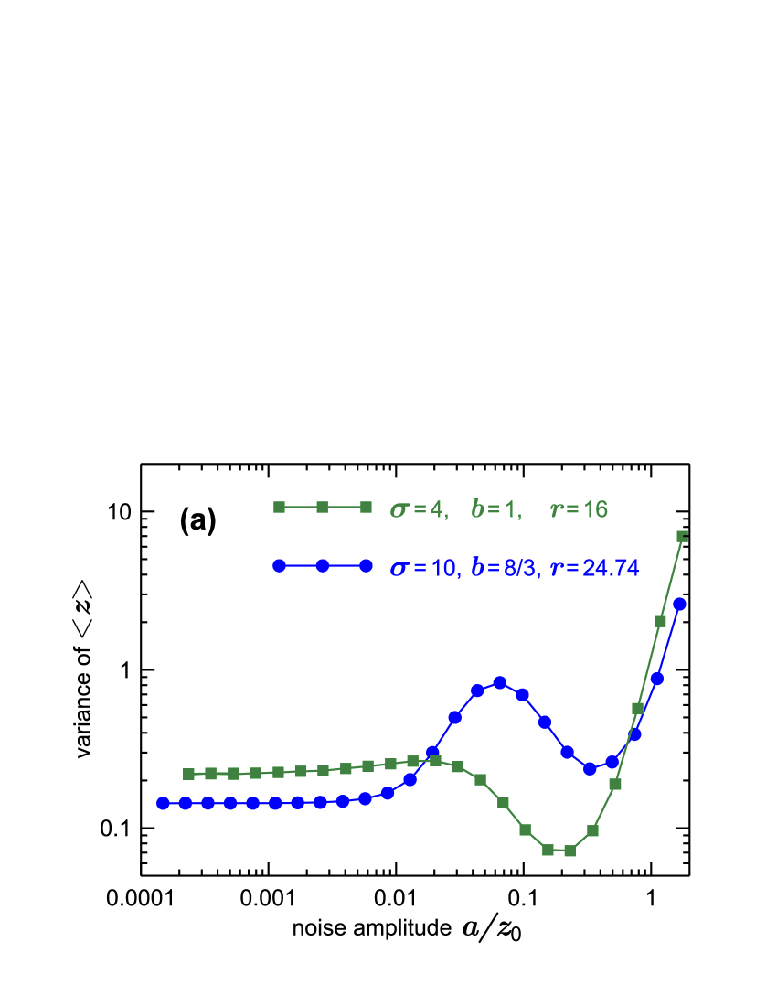
Figure 4: Noise-induced regularization of chaotic dynamics in the Lorenz system at ($\sigma=1$, $b=8/3$, $r=24.74$) and ($\sigma=4$, $b=1$, $r=16$): (a) variance of $\langle{z}\rangle$ calculated over $20$-loop segments of the chaotic orbit and (b) phase diffusion coefficient measuring coherence of chaotic oscillations. Noise amplitude $a$ in graphs is scaled to the coordinate of the saddle points $z_{0}=r-1$.

We performed simulations for the Lorenz system (1) with white Gaussian noise $a\xi(t)$ put into $dz/dt$. We provide here the numerical simulation results for additive noise in order to exclude the trivial deterministic effect of the Stratonovich drift on the system and show the effect manifestation in its pure form. However, the analytical theory constructed is valid both for additive and multiplicative noise. Numerical simulations for several forms of a multiplicative noise with zero Stratonovich drift did not reveal anything new compared to the case of additive noise and we restrict ourselves to presenting the results for the additive noise only. With the laser interpretation of the Lorenz system Oraevskii-1981 , $z$ measures the inversion of the population of energetic levels and is both naturally subject to noise and easily accessible for applying additional additive noise via noise in the energy pumping.

With the classical values of parameters $\sigma=10$ and $b=8/3$, the inhomogeneity of the chaotic set is strongest near the threshold where it becomes attracting, $r\approx 24.06$ (e.g., see Kaplan-Yorke-1979 ; Sparrow-1982 ). At $r\approx 24.74$ the chaotic attractor becomes the only attractor in the phase space (between the stability threshold and this point, it coexists with the stable fixed points which significantly influence the noise-perturbed dynamics of the system). In Fig. 4(a), the dependence of $\mathrm{var}\langle{z}\rangle$ for $20$-loop segments of the chaotic trajectory on the noise amplitude exhibits a well-pronounced minimum and resembles the theoretical dependencies in Fig. 3. Indeed, the dependencies in Fig. 4a may be decomposed into superposition of a stepwise drop (compare to the solid lines in Fig. 3) and quadratic growth of $\mathrm{var}\langle{z_{j}}\rangle$ due to noisy distortion of trajectories; exactly such superpositions form theoretical dependencies plotted in Fig. 3. The disorder-reduction effect for some level of noise is well pronounced though this local minimum corresponds to larger dispersion than in the noise-free case (circle-marked blue curve in the plot). In reality, the level of noise cannot be zero and this local minimum can provide a smaller dispersion than that for the minimal noise level if, for instance, noise cannot be diminished below $a=0.05\,z_{0}$ ($z_{0}=r-1$ is the coordinate of the saddle points). Furthermore, the local minimum can become a global one for a larger inhomogeneity of the attractor. In Fig. 4(a), the dependence of $\mathrm{var}\langle{z}\rangle$ on the noise amplitude for $\sigma=4$, $b=1$, $r=16$ (where the chaotic attractor nearly touches the slightly unstable non-trivial saddle points) has the minimum which provides 3 times smaller dispersion than the noise-free case.

The dispersion of $\langle{z}\rangle$ calculated over finite segments of the chaotic trajectory is only a sample of a quantifier with which one can observe the ordering effect of noise we report. This ordering can be observed with other quantifiers of the system dynamics as well. For instance, one of the very important characteristics of the chaotic systems is the coherence of their oscillations. In particular, coherence determines susceptibility of the system to control forcing and predisposition to synchronization (e.g., see Pikovsky-Rosenblum-Kurths-2001 ; Goldobin-Rosenblum-Pikovsky-2003 ; Goldobin-2008 ). The coherence is quantified by the diffusion coefficient of the chaotic oscillation phase (the oscillation phase to be introduced so that it growths by $2\pi$ for one revolution of the trajectory). In Fig. 4(b) the dependencies of the phase diffusion coefficient on the noise amplitude are plotted for the same sets of parameters as we used for calculation of the dispersion of $\langle{z}\rangle$. One can see well pronounced minima. For $\sigma=4$, $b=1$, $r=16$ the diffusion can be suppressed by factor $5$ in comparison with the noise-free case.

Figure 5: Noise-induced regularization of chaotic dynamics for mapping (11).

5 Observation of the noise-induced regularization effect with mapping

Our analytical treatment is not restricted to the Lorenz system which is utilized only for demonstration. The Lorenz system is known to possess significant peculiarities Sparrow-1982 ; therefore it would be appropriate to validate the effect we observe with independent examples. The classical scenario of the transition to chaos in the Lorenz system is known to be a special case of the transition to chaos via cascade of bifurcations of homoclinic loops Lyubimov-Zaks-1983 . Within the vicinity of the bifurcation accumulation point, a general system, where such a scenario of the transition to chaos occurs, can be described by the following mapping (in the noise-free case) Lyubimov-Zaks-1983 ;

$$x_{n+1} = \left\{\begin{array}[]{cc}x_{n}^{\nu}-\rho_{1}\,,&\mbox{ for }x_{n}>0\,;\\[5.0pt] -A_{2}|x_{n}|^{\nu}+\rho_{2}\,,&\mbox{ for }x_{n}<0\,;\end{array}\right.$$ (7)

$$t_{n+1} = t_{n}+1+\left\{\begin{array}[]{cc}T_{1}\ln(\rho_{1}/x_{n})\,,&\mbox{ for }x_{n}>0\,;\\[5.0pt] T_{2}\ln(\rho_{2}/|x_{n}|)\,,&\mbox{ for }x_{n}<0\,;\end{array}\right.$$ (10)

where $x_{n}$ is the system state at the time moment $t_{n}$, $\nu$ is the saddle index, $\rho_{i}$ are the parameters featuring deviation from the bifurcation accumulation point ($\rho_{1}=\rho_{2}=0$ at this point). The iteration $n\to n+1$ corresponds to the $(n+1)$-th revolution of the system—the oscillation phase grows for $2\pi$ as $n\to n+1$. For the sake of definiteness we restrict ourselves to the case of $\rho_{1}=\rho_{2}\equiv\rho$, $\nu=1/2$, $A_{2}=1$, $T_{1}=T_{2}=1$ and introduce noise:

$$\begin{array}[]{c}\displaystyle x_{n+1}=\mathrm{signum}(x_{n})(\sqrt{|x_{n}|}-\rho)+a\zeta_{n}\,;\\[5.0pt] t_{n+1}=t_{n}+1+\ln(\rho/|x_{n}|).\end{array}$$ (11)

Here $a$ is the noise amplitude and $\zeta_{n}$ are independent random numbers uniformly distributed in $\left[-\sqrt{3},\sqrt{3}\right]$ (i.e., $\langle\zeta^{2}\rangle=1$).

For this mapping the phase grows uniformly with each iteration while time increments $(t_{n+1}-t_{n})$ are non-constant. The phase diffusion can be calculated from $t_{n}$ as a function of $n$ (see, e.g., Reimann-etal-2001 ). In Fig. 5 one can see that the regularizing effect of noise can be as well observed near $\rho=0.25$ where the natural measure distribution is highly inhomogeneous.

6 Conclusion

We have reported the ordering effect of noise on the chaotic dynamics. This effect is rooted into inhomogeneity of the natural measure over the attractor and the fact that noise diminishes this inhomogeneity. Without noise, the measure is determined by the largest multipliers of unstable periodic orbits (UPOs) composing the chaotic attractor and is typically extremely nonuniform for long orbits due to the exponential dependence of the multiplier on the orbit length and the Lyapunov exponent which vary for different UPOs. Generally, the unweighted probability density function of some average for UPOs is centered around the value which does not have to correspond to the maximal measure (see Fig. 1 where the big tail of the weighted PDF clearly indicates that the natural measure of UPOs with large $\langle{z}\rangle$ is drastically larger than that of UPOs near the peak of the unweighted PDF). Hence, the dynamics is more contributed by UPOs which are not “geometrically typical”. Noise smooths the measure over the set of UPOs and reduces the role of excursions along the “untypical” UPOs. On these grounds, we expect the effect to be a universal feature for chaotic dynamics with exception for some model systems with absolutely uniform natural measure (like the tent map). With strong enough inhomogeneity given, the ordering effect can overwhelm the distorting action of noise on UPOs and lead to significant observable ordering of the system dynamics. We have developed the analytical theory for the effect of noise on the measure distribution over chaotic attractor and observed the ordering effects for dispersion of averages over finite segments of the chaotic trajectory and coherence of chaotic oscillations. Noteworthy, the reported phenomenon is novel; its mechanism being robust and vital is not related to any of well-known phenomena of noise-induced ordering (stochastic McNamara-Wiesenfeld-1989 ; Gammaitoni-etal-1998 or coherence resonance Pikovsky-Kurths-1997 , suppression of deterministic chaos by noise Anishchenko-1995 , etc.).

The particular example of potential practical application of the phenomenon discussed is the control of single-mode semiconductor and gas lasers, where increase of the energy pumping (and lasing power) leads to chaotic radio-frequency self-modulation of the amplitude of the laser emission wave Oraevskii-1981 ; Boccaletti-Allaria-Meucci-2004 . Such a modulation of signal might be undesirable as it leads to broadening of the power spectrum and, therefore, difficulties for focusing the laser beam or redirecting it without angular divergence. The decrease of coherence of the amplitude or phase modulation as well impairs opportunities for information transfer and employability of the system for fiber-optics communication. Synchronization phenomena and the coherence property for laser systems also provide opportunities related to cryptography (e.g., see Banerjee-etal-2011a ; Banerjee-etal-2011b ). In general, the coherence determines the precision of clocks (including biological ones Montminy-1997 ; Bell-Pedersen-etal-2005 ), the quality of electric generators, the susceptibility of oscillatory systems to external driving (e.g., see Goldobin-Rosenblum-Pikovsky-2003 ; Goldobin-2008 ) and, therefore, their predisposition to synchronization.

- (1) B. McNamara, K. Wiesenfeld, Theory of stochastic resonance, Phys. Rev. A 39, 4854 (1989).
- (2) L. Gammaitoni, P. Hanggi, P. Jung, F. Marchesoni Stochastic resonance, Rev. Mod. Phys. 70, 223 (1998).
- (3) A.S. Pikovsky, J. Kurths, Coherence resonance in a noise-driven excitable system, Phys. Rev. Lett. 78, 775 (1997).
- (4) V.S. Anishchenko, Chaos structure and properties in the presence of noise, in Dynamical Chaos – Models and Experiments: Appearance Routes and Structure of Chaos in Simple Dynamical Systems, edited by L. O. Chua (World Scientific, 1995), p. 302.
- (5) Ch. Zhou, J. Kurths, I.Z. Kiss, J.L. Hudson, Noise-Enhanced Phase Synchronization of Chaotic Oscillators, Phys. Rev. Lett. 89, 014101 (2002).
- (6) J.N. Teramae, D. Tanaka, Robustness of the Noise-Induced Phase Synchronization in a General Class of Limit Cycle Oscillators, Phys. Rev. Lett. 93, 204103 (2004).
- (7) D.S. Goldobin, A.S. Pikovsky, Synchronization of self-sustained oscillators by common white noise, Physica A 351, 126 (2005).
- (8) D.S. Goldobin, A. Pikovsky, Synchronization and desynchronization of self-sustained oscillators by common noise, Phys. Rev. E 71, 045201(R) (2005).
- (9) D.S. Goldobin, J.-N. Teramae, H. Nakao, G.B. Ermentrout, Dynamics of Limit-Cycle Oscillator Subject to General Noise, Phys. Rev. Lett. 105, 154101 (2010).
- (10) P.W. Anderson, Absence of Diffusion in Certain Random Lattices, Phys. Rev. 109, 1492 (1958).
- (11) J.D. Maynard, Colloquium: Acoustical analogs of condensed-matter problems, Rev. Mod. Phys. 73, 401 (2001).
- (12) D.S. Goldobin, E.V. Shklyaeva, Diffusion of a passive scalar by convective flows under parametric disorder, J. Stat. Mech.: Theory Exp. P01009 (2009).
- (13) D.S. Goldobin, E.V. Shklyaeva, Localization and advectional spreading of convective flows under parametric disorder, J. Stat. Mech.: Theory Exp. P09027 (2013).
- (14) E.G. Altmann, A. Endler, Noise-Enhanced Trapping in Chaotic Scattering, Phys. Rev. Lett. 105, 244102 (2010).
- (15) E.N. Lorenz, Deterministic nonperiodic flow, J. Atmos. Sci. 20, 130 (1963).
- (16) D.V. Lyubimov, M.A. Zaks, Two mechanisms of the transition to chaos in finite-dimensional models of convection, Physica 9D, 52 (1983).
- (17) C. Grebogi, E. Ott, J.A. Yorke, Unstable Periodic Orbits and the Dimensions of Multifractal Chaotic Attractors, Phys. Rev. A 37, 1711 (1988).
- (18) E. Ott, Chaos in Dynamical Systems (University Press, Cambridge, 1993).
- (19) B. Eckhardt, G. Ott, Periodic orbit analysis of the Lorentz attractor, Z. Phys. B 93, 259 (1994).
- (20) M.A. Zaks, D.S. Goldobin, Comment on “Time-averaged properties of unstable periodic orbits and chaotic orbits in ordinary differential equation systems,” Phys. Rev. E 81, 018201(2010).
- (21) P. Cvitanovic, C.P. Dettmann, R. Mainieri, G. Vattay, Trace Formulas for Stochastic Evolution Operators: Weak Noise Perturbation Theory, J. Stat. Phys. 93 (3/4), 981 (1998).
- (22) C.P. Dettmann, T.B. Howard, Asymptotic expansions for the escape rate of stochastically perturbed unimodal maps, Physica D 238, 2404 (2009).
- (23) D. Lippolis, P. Cvitanovic, How Well Can One Resolve the State Space of a Chaotic Map? Phys. Rev. Lett. 104, 014101 (2010).
- (24) P. Gaspard, Trace Formula for Noisy Flows, J. Stat. Phys. 106(1/2), 57 (2002).
- (25) E.G. Altmann, J.C. Leitao, J.V. Lopes, Effect of noise in open chaotic billiards, Chaos 22, 026114 (2012).
- (26) P. Cvitanovic, Chaos: Classical and Quantum (http://chaosbook.org, ver. 14, 2012).
- (27) R. Bowen, On Axiom A Diffeomorphisms, CBMS Regional Conference Series in Mathematics, Vol. 35 (American Mathematical Society, Providence, 1978).
- (28) A.N. Oraevskii, Masers, lasers, and strange attractors, Sov. J. Quantum Electron. 11, 71 (1981).
- (29) J.L. Kaplan, J.A. Yorke, Preturbulence: A regime observed in a fluid flow model of Lorenz, Commun. Math. Phys. 67, 93 (1979).
- (30) C. Sparrow, The Lorenz equations: Bifurcations, chaos, and strange attractors (Springer, 1982).
- (31) A.S. Pikovsky, M. Rosenblum, J. Kurths, Synchronization—A Unified Approach to Nonlinear Science (Cambridge University Press, Cambridge, UK, 2001).
- (32) D. Goldobin, M. Rosenblum, A. Pikovsky, Controlling oscillator coherence by delayed feedback, Phys. Rev. E 67, 061119 (2003).
- (33) D.S. Goldobin, Coherence versus reliability of stochastic oscillators with delayed feedback, Phys. Rev. E 78, 060104(R) (2008).
- (34) P. Reimann, C. van den Broeck, H. Linke, P. Hänggi, J.M. Rubi, A. Pérez-Madrid, Giant Acceleration of Free Diffusion by Use of Tilted Periodic Potentials, Phys. Rev. Lett. 87, 010602 (2001).
- (35) S. Boccaletti, E. Allaria, R. Meucci, Experimental control of coherence of a chaotic oscillator, Phys. Rev. E 69, 066211 (2004).
- (36) S. Banerjee, L. Rondoni, S. Mukhopadhyay, A.P. Misra, Synchronization of spatiotemporal semiconductor lasers and its application in color image encryption, Opt. Commun. 284(9), 2278 (2011).
- (37) S. Banerjee, L. Rondoni, S. Mukhopadhyay, Synchronization of time delayed semiconductor lasers and its applications in digital cryptography, Opt. Commun. 284(19), 4623 (2011).
- (38) M. Montminy, Transcriptional regulation by cyclic AMP, Annu. Rev. Biochem. 66, 807 (1997).
- (39) D. Bell-Pedersen, et al., Circadian rhythms from multiple oscillators: lessons from diverse organisms, Nat. Rev. Genet. 6, 544 (2005).