Monitoring Entanglement Evolution and Collective Quantum Dynamics

Abstract

We generalize a recently developed scheme for monitoring coherent quantum dynamics with good time-resolution and low backaction [Reuther et al., Phys. Rev. Lett. 102, 033602 (2009)] to the case of more complex quantum dynamics of one or several qubits. The underlying idea is to measure with lock-in techniques the response of the quantum system to a high-frequency ac field. We demonstrate that this scheme also allows one to observe quantum dynamics with many frequency scales, such as that of a qubit undergoing Landau-Zener transitions. Moreover, we propose how to measure the entanglement between two qubits as well as the collective dynamics of qubit arrays.

I Introduction

A most fascinating question in quantum mechanics is how much a measurement acts back on a quantum system and thus influences the state of the latter. Walls and Milburn (1995); Nielsen and Chuang (2000); Breuer and Petruccione (2002) According to the classic measurement postulate, the projective measurement of a quantity causes a collapse of the wave function into an eigenstate of the corresponding operator. However, quantum mechanics only allows probabilistic statements about the state into which the wave function collapses. This evolution into a mixture can be modeled by coupling the quantum system via the measurement operator to a measurement apparatus, i.e., to a macroscopic environment which provokes dissipation and decoherence. A natural interpretation of this process is that information about the quantum system leaks into the environment, while the system acquires entropy. Since the environment is perceived as classical object, one may assume that the pointer of a measurement apparatus corresponds to a collective environment coordinate. Zurek (2003) Then the question arises how the quantum system and this collective coordinate influence each other. In other words, which information about the quantum system is contained in the collective coordinate and how strong is the backaction of the environment on the system?

A specific example for such a measurement device is a low-frequency “tank circuit” coupled to a superconducting qubit. Grajcar et al. (2004); Sillanpää et al. (2005) Here, one makes use of the fact that the resonance frequency of the oscillator depends on the qubit state which, in turn, influences the phase of the oscillator response. This allows one to measure both the charge and the flux degree of freedom of superconducting qubits. The drawback of this scheme, however, is that the coherent qubit dynamics is considerably faster than the driving. Thus, one can only observe the time-average of the qubit state, but not time-resolve its dynamics. Measuring the qubit directly by driving it at resonance is possible as well. Ya. S. Greenberg et al. (2005) This however induces Rabi oscillations and, thus, alters the qubit dynamics significantly. Liu et al. (2006); Wilson (2007).

In Ref. Reuther et al., 2009, we proposed to probe a quantum system with a weak high-frequency drive acting directly upon the qubit. We found that the reflected signal possesses a time-dependent phase shift which is related to a qubit observable. This relation was validated for a Cooper-pair box that is in a superposition of the two lowest energy eigenstates which form a qubit. In particular, it was shown that coherent oscillations of this qubit are visible in the reflected signal, while the driving-induced backaction stays at a tolerable level. This enables time-resolved monitoring of the coherent qubit dynamics.

In this article we demonstrate that this measurement scheme is applicable also to more complex quantum dynamics, and even the evolution of entanglement between two qubits can be observed in this way. In Sec. II, we introduce the underlying system-bath model and describe how we quantify measurement fidelity and backaction. Moreover, we derive a relation between the reflected ac signal and the monitored time-dependent expectation value of the quantum system. This relation, which constitutes our measurement scheme, is numerically tested in Sec. III for the case of a qubit undergoing Landau-Zener sweeps. In Sec. IV, we present a protocol for monitoring entanglement between two qubits. Finally, we derive in Sec. V how the collective dynamics of a qubit array enhances the signal.

II High-frequency response of a quantum system

II.1 System-bath model

We consider a quantum system interacting with a dissipative environment, as depicted in Fig. 1. The system-bath Hamiltonian is given by Leggett et al. (1987); Hänggi et al. (1990); Makhlin and Mirlin (2001)

$$H=H_{0}+\sum_{k}\Big{(}\frac{\varphi_{k}^{2}}{2L_{k}}+\frac{(q_{k}-\lambda_{k}Q/\omega_{k})^{2}}{2C_{k}}\Big{)}\;.$$ (1)

Here, $H_{0}$ denotes the system Hamiltonian and $Q$ is the system operator that couples to the environment. To be specific, we assume that $Q$ is the system excess charge. In the realm of circuit QED, the bath is typically modeled by a transmission line in terms of $LC$ circuits with charges $q_{k}$ and conjugate fluxes $\varphi_{k}$, where $C_{k}$ and $L_{k}$ are effective capacitances and inductances, respectively. Furthermore, $\omega_{k}=(L_{k}C_{k})^{-1/2}$ denotes the angular frequency of mode $q_{k}$, and $\lambda_{k}$ are the corresponding coupling constants in units of frequencies. The system-bath interaction is fully characterized by the spectral density

$$I(\omega)=\frac{\pi}{2}\sum_{k}\lambda_{k}^{2}\sqrt{\frac{L_{k}}{C_{k}}}\,\delta(\omega-\omega_{k})\;,$$ (2)

which is assumed to be ohmic with an effective impedance $Z_{0}$, i.e. $I(\omega)=\omega Z_{0}$. Yurke and Denker (1984); Devoret (1995); Makhlin and Mirlin (2001) Assuming a weak system-bath interaction, we obtain the Bloch-Redfield master equation for the reduced system density operator $\rho$ by standard techniques, Fonseca-Romero et al. (2005); Grifoni and Hänggi (1998)

$$\dot{\rho}=\mathcal{L}_{0}\rho=-\frac{i}{\hbar}[H_{0},\rho]-\frac{1}{\hbar}[Q,[\hat{Q},\rho]]-i\frac{Z_{0}}{\hbar}[Q,[\dot{Q},\rho]_{+}],$$ (3)

where $[A,B]_{+}=AB+BA$ denotes the anticommutator, $\dot{Q}=i[H_{0},Q]/\hbar$ and

$$\hat{Q}=\frac{1}{\pi}\int_{0}^{\infty}d\tau\int_{0}^{\infty}d\omega\,S(\omega)\cos(\omega\tau)\tilde{Q}(-\tau).$$ (4)

Here, $S(\omega)=I(\omega)\coth(\hbar\omega/2k_{\rm B}T)$ denotes the Fourier transformed of the symmetrically ordered equilibrium bath correlation function at temperature $T$. The shorthand notation $\tilde{X}(t)$ represents the interaction-picture operator $U_{0}^{\dagger}(t)XU_{0}(t)$, where $U_{0}$ denotes the system propagator.

II.2 Input-output formalism

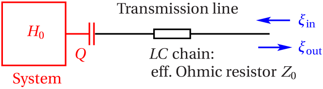
Figure 1: (Color online) Sketch of the input-output formalism: A quantum system described by a Hamiltonian $H_{0}$ is coupled via its charge degree of freedom $Q$ to an environment in form of a transmission line with ohmic effective impedance $Z_{0}$. When the system is probed by an input signal $\xi_{\mathrm{in}}$, the output signal $\xi_{\mathrm{out}}$ contains information about the bare system dynamics.

The central concept of our measurement scheme is to relate the quantum dynamics of the externally probed central circuit to a response via the transmission line. In order to quantify the response, we employ the input-output formalism. Gardiner and Collett (1985); Johansson et al. (2006) We start from the Heisenberg equation of motion (operator label $H$) for the environmental mode $k$,

$$\ddot{q}_{k}^{H}+\omega_{k}^{2}q_{k}^{H}=\lambda_{k}\omega_{k}Q^{H}\;,$$ (5)

which is linear in the bath operators. Its formal solution for initial time $t_{0}=0$ reads

$$q_{k}^{H}(t)=q_{k}(0)\cos(\omega_{k}t)+\sqrt{\frac{C_{k}}{L_{k}}}\varphi_{k}(0)\sin(\omega_{k}t)\\ +\lambda_{k}\int_{0}^{t}d\tau\sin[\omega_{k}(t-\tau)]Q^{H}(\tau)\;.$$ (6)

It depends on the history of the system, which gets expressed through the convolution integral in the second line of Eq. (6). Inserting the obtained solution into the Heisenberg equation of motion for any system observable $X$ yields

$$\begin{split}\dot{X}^{H}=&\frac{i}{\hbar}\left[H_{0}^{H},X^{H}\right]+\frac{i}{\hbar}\left[\left(Q^{H}\right)^{2},X^{H}\right]\sum_{k}\sqrt{\frac{L_{k}}{C_{k}}}\frac{\lambda_{k}^{2}}{2\omega_{k}}\\ &-\frac{i}{\hbar}\left[Q^{H},X^{H}\right]\sum_{k}\lambda_{k}^{2}\sqrt{\frac{L_{k}}{C_{k}}}\\ &\times\int_{0}^{t}d\tau\sin[\omega_{k}(t-\tau)]Q^{H}(\tau)-\frac{i}{\hbar}[Q^{H},X^{H}]\\ &\times\sum_{k}\lambda_{k}\left(\sqrt{\frac{L_{k}}{C_{k}}}q_{k}(0)\cos(\omega_{k}t)+\varphi_{k}(0)\sin(\omega_{k}t)\right).\end{split}$$ (7)

At this point we define the operator

$$\xi_{\mathrm{in}}^{\mathrm{qm}}(t)=\sum_{k}\lambda_{k}\left(\sqrt{\frac{L_{k}}{C_{k}}}q_{k}(0)\cos(\omega_{k}t)+\varphi_{k}(0)\sin(\omega_{k}t)\right)\;,$$ (8)

which allows a convenient notation. It is fully determined by the bath correlation function and, following the above equation of motion, Eq. (7), only depends on the environment operators at initial time. Therefore, it can be interpreted as a signal entering via the transmission line, i.e. describes the input noise acting upon the system.

After a partial integration of the third term of Eq. (7), the counter-term proportional to $[(Q^{H})^{2},X^{H}]$ is canceled. Furthermore, for the ohmic spectral density $I(\omega)=\omega Z_{0}$, Eq. (7) becomes local in time, and one arrives at the quantum Langevin equation Ford et al. (1988); Hänggi et al. (2005); Hänggi and Marchesoni (2009)

$$\dot{X}^{H}=\frac{i}{\hbar}\left[H_{0}^{H},X^{H}\right]-\frac{iZ_{0}}{\hbar}\left[Q^{H},X^{H}\right]\dot{Q}^{H}\\ -\frac{i}{\hbar}[Q^{H},X^{H}]\xi_{\mathrm{in}}^{\mathrm{qm}}(t)\;.$$ (9)

It contains the input field $\xi_{\text{in}}^{\mathrm{qm}}(t)$ and an ohmic dissipative term $\propto Z_{0}\dot{Q}^{H}$.

It is also possible to express the quantum Langevin equation in terms of the outgoing fluctuations. This can be achieved by solving Eq. (5) for the bath modes starting at a later time $t_{1}>t$. The solution is the time-reversed counterpart of Eq. (6) and reads

$$q_{k}^{H}(t)=q_{k}(t_{1})\cos[\omega_{k}(t-t_{1})]+\sqrt{\frac{C_{k}}{L_{k}}}\varphi_{k}(t_{1})\sin[\omega_{k}(t-t_{1})]\\ -\lambda_{k}\int_{t}^{t_{1}}d\tau\sin[\omega_{k}(t-\tau)]Q^{H}(\tau)\;.$$ (10)

According to Eq. (8), we define the sum over all modes $k$ with respect to the first two terms of Eq. (10) as the outgoing noise $\xi_{\mathrm{out}}^{\mathrm{qm}}(t)$. In contrast to $\xi_{\text{in}}^{\mathrm{qm}}(t)$, it is influenced by the system at earlier times $t<t_{1}$ and, thus, contains information about the system dynamics. Gardiner and Collett (1985) Proceeding as above, we obtain the time-reversed Langevin equation

$$\dot{X}^{H}=\frac{i}{\hbar}\left[H_{0}^{H},X^{H}\right]\\ +\frac{iZ_{0}}{\hbar}\left[Q^{H},X^{H}\right]\dot{Q}^{H}-\frac{i}{\hbar}[Q^{H},X^{H}]\xi_{\mathrm{out}}^{\mathrm{qm}}(t)\;.$$ (11)

Its characteristic is a negative damping term, i.e., it is formally obtained from the quantum Langevin equation (9) via the substitution $Z_{0}\rightarrow-Z_{0}$. This corresponds to backward propagation in time, as Eq. (11) only accounts for the environment at later times $t_{1}>t$.

The difference between the two Langevin equations relates the input to the output fluctuations as Gardiner and Collett (1985)

$$\xi_{\text{out}}^{\mathrm{qm}}(t)-\xi_{\text{in}}^{\mathrm{qm}}(t)=-2Z_{0}\dot{Q}^{H}=-\frac{2iZ_{0}}{\hbar}\big{[}H_{0}^{H},Q^{H}\big{]}.$$ (12)

The last equality has been obtained from the Heisenberg equation of the charge operator, $\dot{Q}^{H}=(i/\hbar)[H_{0}^{H},Q^{H}]$, which is independent of the environment since $Q$ commutes with the system-bath coupling Hamiltonian. Equation (12) determines the influence of the system on its environment and, thus, represents the central relation of the input-output formalism. At this stage, it is worth emphasizing the environment possesses many degrees of freedom which all acquire information about the quantum system. Therefore, the collective bath coordinates $\xi_{\text{in/out}}^{\mathrm{qm}}(t)$ are classical in the sense that their expectation values can be interpreted as the outcome of a single measurement. Zurek (2003)

II.3 Response to high-frequency driving

The central idea of our scheme is to excite the system by a classical ac drive and to measure the resulting system response. Physically, the driving enters like the quantum noise via the transmission line. Therefore, it can be modelled as a coherently and highly excited bath mode in the classical limit weakly coupled to the system. Grifoni and Hänggi (1998) This means that the input fluctuations are augmented by a deterministic ac contribution. Thus, they become $\xi_{\mathrm{in}}(t)=\xi_{\mathrm{in}}^{\mathrm{qm}}(t)+A\cos(\Omega t)$ and, accordingly, $\xi_{\mathrm{out}}(t)=\xi_{\mathrm{out}}^{\mathrm{qm}}(t)+A\cos(\Omega t)$. The deterministic terms also affects the input-output relation (12) which now reads

$$\xi_{\text{out}}(t)=\xi_{\mathrm{in}}^{\mathrm{qm}}(t)+A\cos(\Omega t)-\frac{2iZ_{0}}{\hbar}[H_{0}^{H},Q^{H}]\,.$$ (13)

In the corresponding expectation value, where we return to the Schrödinger picture for convenience, the fluctuation $\xi_{\mathrm{in}}^{\mathrm{qm}}$ vanishes, such that,

$$\langle\xi_{\text{out}}(t)\rangle=A\cos(\Omega t)-\frac{2iZ_{0}}{\hbar}\langle[H_{0},Q]\rangle_{t}\,.$$ (14)

This expresses the expectation value of the output field in terms of the input field and a system expectation value, $\langle\ldots\rangle_{t}=\mathrm{tr}[\rho(t)\ldots]$. The latter contains information about the system dynamics and is the central quantity of interest.

The quantum Langevin equations (9) and (11) have been convenient for deriving the relations between the input and the output fields, Eqs. (12) and (13). For the actual computation of the system expectation value on the r.h.s. of Eq. (14), by contrast, such stochastic, operator-valued equations are less practical. Therefore, we derive in addition an equivalent quantum master equation which not only serves for numerical computations, but will also provide an analytical high-frequency approximation.

We start by noticing that a classical ac drive $A\cos(\Omega t)$ coupled to the system charge $Q$ corresponds to a Hamiltonian $QA\cos(\Omega t)$. Thus, the system Hamiltonian $H_{0}$ has to be replaced by

$$H(t)\equiv H_{0}+QA\cos(\Omega t)\;.$$ (15)

A key requirement of our measurement scheme is that the driving must not significantly alter the system dynamics. Thus, we assume that the amplitude $A$ is sufficiently small, which allows us to treat the driving perturbatively. Kohler et al. (1997) In doing so, we use the ansatz $\rho(t)=\rho_{0}(t)+\rho_{1}(t)$, where $\rho_{0}(t)$ describes the dynamics of the system without ac driving, and $\rho_{1}(t)$ denotes the correction to the system state. With this ansatz, the master equation reads

$$\dot{\rho}(t)=\big{[}\mathcal{L}_{0}+\mathcal{L}_{1}(t)\big{]}\big{[}\rho_{0}(t)+\rho_{1}(t)\big{]}\;,$$ (16)

where the perturbative driving manifests in the Liouvillian

$$\mathcal{L}_{1}(t)\rho(t)=-\frac{i}{\hbar}A[Q,\rho(t)]\cos\Omega t\,,$$ (17)

To lowest order in $A$, the correction $\rho_{1}$ obeys

$$\dot{\rho}_{1}(t)=\mathcal{L}_{0}\rho_{1}(t)-\frac{i}{\hbar}A[Q,\rho_{0}(t)]\cos(\Omega t)\;.$$ (18)

This linear inhomogeneous equation of motion can be solved formally in terms of a convolution between the propagator of the undriven system and the inhomogeneity,

$$\rho_{1}(t)=e^{\mathcal{L}_{0}t}\rho_{1}(0)-\frac{i}{\hbar}\int\limits_{0}^{\;t}d\tau\,e^{\mathcal{L}_{0}(t-\tau)}A[Q,\rho_{0}(\tau)]\cos(\Omega\tau)\;,$$ (19)

with $\rho_{1}(0)=0$. If the driving frequency $\Omega$ is much larger than all relevant system frequencies, the integral can be simplified by time-scale separation: First, we split the above integral into a sum of integrals over complete periods and a final one over the remaining time. Assuming that the slow $\rho_{0}(t)$ is practically constant during one oscillation period of $2\pi/\Omega$, the integrals over complete driving periods vanish, while the last contribution can be evaluated using $\rho_{0}(\tau)\approx\rho_{0}(t)$. In this way, we obtain the solution for the time evolution of the reduced density matrix

$$\rho(t)=\rho_{0}(t)-\frac{iA}{\hbar\Omega}[Q,\rho_{0}(t)]\sin(\Omega t)\;,$$ (20)

where $eA/\hbar\Omega$ is identified as the necessarily small perturbation parameter. Within this approximation for the density operator, the expectation value of the output, Eq. (14), becomes

$$\langle\xi_{\text{out}}(t)\rangle=A\cos(\Omega t)-\frac{2iZ_{0}}{\hbar}\langle[H_{0},Q]\rangle_{0,t}\\ +\frac{2AZ_{0}}{\hbar^{2}\Omega}\left\langle[[H_{0},Q],Q]\right\rangle_{0,t}\sin(\Omega t)\;,$$ (21)

where the subscript in $\langle\ldots\rangle_{0,t}=\mathrm{tr}[\rho_{0}(t)\ldots]$ refers to the undriven dynamics.

At this point we note that $\langle\xi_{\text{out}}(t)\rangle$ contains both low-frequency components stemming from the pure system dynamics as well as high-frequency components induced by the external driving. The latter corresponds to the second term of Eq. (20). Now, in an experiment, it is feasible to single out the high-frequency components of the outgoing signal using a lock-in technique, where the incoming signal represents the reference oscillator. This removes the second term on the r.h.s. of Eq. (21), such that the outgoing signal becomes

$$\langle\xi_{\text{out}}^{\mathrm{hf}}(t)\rangle=A\cos(\Omega t)+\frac{2AZ_{0}}{\hbar^{2}\Omega}\left\langle[[H_{0},Q],Q]\right\rangle_{0,t}\sin(\Omega t).$$ (22)

Since the second term is a perturbative correction, it has to be small so that Eq. (22) can be written as

$$\langle\xi_{\text{out}}^{\mathrm{hf}}(t)\rangle=A\cos[\Omega t-\phi_{\mathrm{hf}}^{0}(t)]$$ (23)

with the time-dependent phase shift

$$\phi_{\mathrm{hf}}^{0}(t)=\frac{2Z_{0}}{\hbar^{2}\Omega}\left\langle[[H_{0},Q],Q]\right\rangle_{0,t}\;.$$ (24)

This relation constitutes the basis of our measurement scheme. It connects a phase shift $\phi^{0}_{\mathrm{hf}}(t)$ between the high-frequency input and the output signals to the low-frequency dynamics of a system observable. In other words, Eq. (24) enables time-resolved monitoring of an open quantum system by measuring the phase shift $\phi^{0}_{\mathrm{hf}}(t)$ with lock-in techniques. We emphasize that our measurement scheme is rather generic and can in principle be applied to any open quantum system.

It is important to note that there are situations in which the phase shift $\phi_{\mathrm{hf}}^{0}(t)$ is independent of the system dynamics or even vanishes. The latter is obviously the case when $Q$ commutes with the system Hamiltonian. A constant phase shift is obtained for an harmonic oscillator $H_{0}=\hbar\omega_{0}(a^{\dagger}a+1/2)$ that couples via its position, i.e., $Q\propto a+a^{\dagger}$, as one easily obtains by evaluating the double commutator in Eq. (24). This is evident from the superposition principle which holds for a linearly driven harmonic oscillator. However, already a coupling $Q\propto(a+a^{\dagger})^{2}$ is sufficient for obtaining a non-trivial response.

II.4 Measurement fidelity and backaction

As broached above, the relation between the phase of the output signal and a system observable relies on a high-frequency approximation. In an experiment, the driving frequency is finite, however. Thus, the experimentally obtained phase $\phi_{\text{out}}^{\text{exp}}(t)$, which is actually recorded by the lock-in amplifier, may differ from the theoretically predicted phase $\phi^{0}_{\text{hf}}(t)\propto\langle[[H_{0},Q],Q]\rangle_{0,t}$. During lock-in amplifying, the high-frequency components of $\langle\xi_{\text{out}}^{\text{hf}}(t)\rangle$, and with it $\phi_{\text{out}}^{\text{exp}}(t)$, are extracted from the output signal $\langle\xi_{\text{out}}(t)\rangle$, where the classical incoming signal $\langle\xi_{\text{in}}(t)\rangle=A\cos(\Omega t)$ serves as the reference oscillator.

Thus, it is crucial to test with a numerical simulation how well both phases agree in a realistic case. As a criterion, we employ the measurement fidelity which we define as the normalized overlap

$$F= \Big{(}\phi_{\text{out}}^{\text{exp}},\phi_{\text{hf}}^{0}\Big{)}$$

$$\equiv \left(\int dt\,[\phi_{\text{out}}^{\text{exp}}(t)]^{2}\int dt\,[\phi^{0}_{\text{hf}}(t)]^{2}\right)^{-1/2}$$

$$\times\Big{|}\int dt\,\phi^{\text{exp}}_{\text{out}}(t)\,\phi^{0}_{\text{hf}}(t)\Big{|}\;,$$ (25)

with time integration over the duration of the measurement. The ideal value $F=1$ corresponds to the case of perfect proportionality between the measured phase $\phi_{\mathrm{out}}^{\text{exp}}(t)$ and $\phi_{\text{hf}}^{0}(t)\propto\langle[[H_{0},Q],Q]\rangle_{0,t}$. Note that $\phi_{\text{hf}}^{0}(t)$ is computed in the absence of the ac driving, while $\phi_{\text{out}}^{\text{exp}}(t)$ is obtained in its presence. Moreover, we have to mimic the action of the lock-in amplifier numerically, as described in Sec. III in the second paragraph after Eq. (32).

Furthermore, for any quantum measurement, one has to worry about backaction on the system in terms of decoherence. In our measurement scheme, decoherence plays a particular role, because both the driving and the ohmic environment couple to the central system via the same mechanism. This is reflected by the fact that the predicted phase of Eq. (24) is proportional to the dissipation strength $Z_{0}$. In terms of the generalized, dimensionless dissipation strength $\alpha=e^{2}Z_{0}/\hbar$, it is required that $\alpha\lesssim 0.1$ in order to preserve a predominantly coherent time evolution. In this context, our measurement is weak, but yet destructive in the sense that it relies on the naturally provided interaction with a dissipative environment causing decoherence. This marks a significant difference to conventional quantum non-demolition (QND) measurement schemes. Walls and Milburn (1995); Breuer and Petruccione (2002) Here by contrast, the additional decoherence due to the driving is minor. This is obvious from the fact that within first-order approximation the system purity is not affected,

$$\mathrm{Tr}(\rho^{2})=\mathrm{Tr}(\rho_{0}^{2})\,,$$ (26)

which follows readily from Eq. (20). Only in this sense, our measurement scheme can be considered as being of non-demolition character.

As a concrete measure for how much the driving perturbs the system, we use in our numerical investigations the time average $\mathrm{bar}D$ of the trace distance Nielsen and Chuang (2000)

$$D(t)=\frac{1}{2}\mathrm{Tr}|\rho(t)-\rho_{0}(t)|\;.$$ (27)

In the ideal case, $\mathrm{bar}D$ vanishes, while $\mathrm{bar}D=1$ if both density operators are completely unrelated.

III Monitoring Landau-Zener sweeps

In Ref. Reuther et al., 2009, we investigated the quality of our measurement scheme using the dynamics of a decaying qubit state as an elementary example. Here, we go a step further and demonstrate that it is applicable to more complex coherent dynamics.

As an example, we consider a Landau-Zener tunneling process between the states of a charge qubit prepared in a Cooper-pair box (CPB), Wendin and Shumeiko (2006); Shevchenko et al. (2010) a paradigmatic example of complex quantum dynamics in a seemingly simple system. In particular, it can be used for state preparation Saito et al. (2006); Zueco et al. (2010) and entanglement generation Wubs et al. (2007); Zueco et al. (2008) in a qubit-resonator system. In recent experiments Oliver et al. (2005); Sillanpää et al. (2006) multiple Landau-Zener sweeps were performed with a charge qubit coupled to a low-frequency tank oscillator whose resonance frequency depends on the time-averaged qubit state. This enabled the measurement of the accumulated phase which determines the qubit state. Here by contrast, we demonstrate that a time-resolved observation of the complex dynamics during a single Landau-Zener transition is possible as well.

We employ the CPB Hamiltonian

$$H_{0}^{\mathrm{CPB}}=4E_{\mathrm{C}}(\hat{N}-N_{g})^{2}-\frac{\delta}{2}\sum_{N=-\infty}^{\infty}(|N{+}1\rangle\langle N|+\text{h.c.}),$$ (28)

where $N$ is the number of excess Cooper pairs in the box. The charge operator reads $Q=2e\hat{N}=2e\sum_{N}N|N\rangle\langle N|$ with $e$ being the elementary charge. The charging energy $E_{\mathrm{C}}$ is determined by the various capacitances of the CPB, while the scaled gate voltage $N_{g}$ and the effective Josephson energy $\delta$ are controllable. If the charging energy is sufficiently large, and $N_{g}$ approaches a charge degeneracy point determined by the half-integer value $N_{g}^{\mathrm{deg}}\approx N_{0}-1/2$, for some integer number $N_{0}$, only the two lowest charge states $|N_{0}-1\rangle\equiv|{\downarrow}\rangle$ and $|N_{0}\rangle\equiv|{\uparrow}\rangle$ matter and form a qubit, while the energy gap to the higher charge states is much larger than the qubit splitting. Makhlin and Mirlin (2001); Vion et al. (2002); Grajcar et al. (2004) In the two-level approximation, the qubit is described by the Hamiltonian

$$H_{0}^{\mathrm{qb}}=-\frac{1}{2}\epsilon\sigma_{z}-\frac{1}{2}\delta\sigma_{x}\,.$$ (29)

The Pauli matrices $\sigma_{i}$ are defined in the qubit subspace and $\epsilon=8E_{\mathrm{C}}(N_{0}-N_{g})$, where $N_{g}$ ranges in the interval $[N_{0}-1,N_{0}]$, is the effective qubit bias. Moreover, $Q_{\mathrm{qb}}=e\sigma_{z}$ while by virtue of relation (24) the phase of the output signal is linked to the qubit observable $\sigma_{x}$ according to

$$\phi_{\mathrm{hf}}^{0}(t)=-\frac{4e^{2}Z_{0}\delta}{\hbar^{2}\Omega}\left\langle\sigma_{x}\right\rangle_{0,t}\,.$$ (30)

Thus, the high-frequency component of $\langle\dot{Q}\rangle$, which is manifest in the phase of the outgoing signal (12), contains information about the low-frequency qubit dynamics in terms of the unperturbed $\langle\sigma_{x}\rangle_{0}$. It is worth mentioning that the preceding discussion equally applies to the case of a flux or phase qubit with an inductive coupling to the transmission line.

The qubit undergoes a Landau-Zener transition when the gate voltage in terms of the background charge $N_{g}$ in the Hamiltonian (28) is swept from a large positive to a negative finite value through the charge degeneracy point at $N_{g}^{\mathrm{deg}}$ with constant velocity, $N_{g}(t)=N_{g}^{0}+v_{g}t$. Accordingly, the qubit Hamiltonian (29) depends on time and can be written as

$$H_{0}(t)=-\frac{v(t-t_{0})}{2}\sigma_{z}-\frac{\delta}{2}\sigma_{x}\,,$$ (31)

where we have defined $v=8E_{C}v_{g}$ and $t_{0}=-N_{g}^{0}/v_{g}$. Hamiltonian (31) is a valid approximation on condition that the sweep ends timely prior to a subsequent anti-crossing in the CPB spectrum.

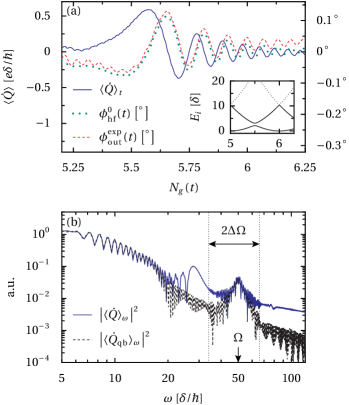
Figure 2: (Color online) Monitoring the dynamics of a dissipative Landau-Zener sweep of a qubit, which is initiated in a weakly probed CPB with $N_{\mathrm{s}}=12$ states operated at $N_{0}=6$. The selected anticrossing lies at $N_{g}=N_{0}-1/2=5.5$, and the initial qubit state is $|{N=5}\rangle\equiv|{\uparrow}\rangle$, while $|{\downarrow}\rangle\equiv|{N=6}\rangle$. The other parameters are $E_{c}=2.6\,\delta$, $v_{g}=0.125\,\delta/\hbar$, $A=\delta/e$, $\alpha=0.05$, and $\Omega=50\,\delta/\hbar$. (a) Time evolution of the output signal $\langle\dot{Q}\rangle_{t}\propto\langle\xi_{\mathrm{out}}(t)\rangle-\langle\xi_{\mathrm{in}}(t)\rangle$ of the full CPB, and its lock-in amplified phase $\phi_{\text{out}}^{\text{exp}}(t)$ (frequency window $\Delta\Omega=16\delta$), compared to the estimated phase $\phi_{\mathrm{hf}}^{0}(t)\propto\langle\sigma_{x}\rangle_{0,t}$ in the qubit approximation. Fast oscillations with frequency $\Omega=50\delta/\hbar$ stemming from the input signal are barely resolved. The inset shows the three lowest CPB eigenenergies as a function of $N_{g}(t)$. (b) Power spectrum of $\langle\dot{Q}\rangle$ for the driven systems, comparing the full CPB Hamiltonian (solid) and in two-level approximation (dashed).

Even if the qubit approximation describes the CPB faithfully for large charging energies, $E_{c}\gg\delta$, one must take into account excitations of higher charge states by the ingoing signal; see also the discussions in Ref. Reuther et al., 2009. In our simulations, we operate at $N_{0}=6$ and truncate the CPB Hilbert space at $N_{\mathrm{s}}=12$ states, which turned out to be sufficient to reach numerical convergence.

Figure 2(a) illustrates the time evolution of the CPB observable

$$\dot{Q}=\frac{ie\delta}{\hbar}\sum_{N=-\infty}^{\infty}(|N\rangle\langle N+1|-|N+1\rangle\langle N|)\;,$$ (32)

during a Landau-Zener transition between the two lowest states; see inset of Fig. 2(a). Within two-level approximation, this operator reads $\dot{Q}=(-e\delta/\hbar)\sigma_{y}$. The parameters are chosen such that the final populations of the two states are roughly equal, because in this crossover regime between the adiabatic and the non-adiabatic dynamics, coherent oscillations are most pronounced. Note that since we plot the time derivative of the charge, $\langle\dot{Q}\rangle\propto\langle\sigma_{y}\rangle$, the final population of the upper state, $[1+\langle\sigma_{z}\rangle(t\rightarrow\infty)]/2$, given by the Landau-Zener probability $P_{\mathrm{LZ}}=\exp(-\pi\delta^{2}/2\hbar v)\approx 0.546$, is not part of the information depicted in Fig. 2(a).

The backaction of the weak driving signal on the system dynamics in terms of a weak modulation of $\langle\dot{Q}\rangle_{t}$ is barely visible. The associated spectrum in terms of $\langle\dot{Q}\rangle_{\omega}$, depicted in panel (b), nevertheless reflects the driving in terms of a small peak at the driving frequency $\Omega=50\delta/\hbar$. Due to the time-dependent qubit splitting, the spectrum exhibits a broad range of frequencies centered at zero, reflected in the sideband structure around $\Omega$. In the time domain these sidebands correspond to a signal $\langle\xi_{\mathrm{out}}^{\mathrm{hf}}(t)\rangle=A\cos[\Omega t-\phi_{\mathrm{out}}^{\text{exp}}(t)]$.

As is indicated above in Secs. II.3 and II.4, the phase $\phi_{\mathrm{out}}^{\text{exp}}(t)$ can be retrieved by lock-in amplification of the output signal in an experiment. We mimic this procedure numerically in the following way: Scofield (1994) We only consider the spectrum of $\langle\xi_{\text{out}}(t)\rangle$ in a frequency window $\Omega\pm\Delta\Omega$ around the driving frequency and shift it by $-\Omega$ in order to center it at zero. The inverse Fourier transformation of the spectrum cutout to the time domain yields the time-dependent phase $\phi_{\mathrm{out}}^{\text{exp}}(t)$ which is expected to agree with $\phi_{\text{hf}}^{0}(t)$; see the discussion in Sec. II.4. According to Eq. (24), this phase reflects the unperturbed time evolution of $\langle\sigma_{x}\rangle_{0}$ with respect to the qubit.

Figure 2(a) shows that the numerically extracted phase $\phi_{\mathrm{out}}^{\text{exp}}(t)$ is indeed in a very good agreement with $\phi^{0}_{\text{hf}}(t)\propto\langle\sigma_{x}\rangle_{0,t}$ for an appropriate choice of parameters. This holds even if the condition of high-frequency probing, i.e. $\Omega$ exceeding all relevant system frequencies by far, is not strictly fulfilled. Appropriate values for $\Omega$ need to be determined from the width of the sideband distributions. These can be estimated from the duration $\tau_{\mathrm{LZ}}$ of a Landau-Zener transition which is $\tau_{\mathrm{LZ}}\approx 20\hbar/\delta$ here. Consequently, the spectral peak has the width $v\tau_{\text{LZ}}/\hbar\approx 20\delta/\hbar$. Thus, in order to avoid any overlap between both distributions, the driving frequency must fulfill $\Omega\gg 20\delta/\hbar$. In the present case, Eqs. (22) and (24) are corroborated already for $\Omega\approx 50\delta/\hbar$.

Furthermore, we require small dissipation, $\alpha\lesssim 0.1$, to keep the time evolution predominantly coherent. In this context, one needs to take care of the interplay of decoherence and the external sweep velocity and its impact on the LZ probability and dynamics. Wubs et al. (2006); Zueco et al. (2008); Nalbach and Thorwart (2009)

Towards the end of the sweep, one notices a deviation between the predicted phase $\phi^{0}_{\text{hf}}(t)$ and $\phi_{\text{out}}^{\text{exp}}(t)$ which becomes curved upward. This stems from the presence of higher charge states, which get slightly populated as soon as $N_{g}$ reaches the next half-integer value $N_{g}^{\mathrm{deg}}+1$, that is, the subsequent avoided level anticrossing in the CPB spectrum. Accordingly, as visible in Fig. 2(b), the spectrum $\langle\dot{Q}\rangle_{\omega}$ contains more pronounced frequency components than the one of the two-level approximation $\langle\dot{Q}_{\mathrm{qb}}\rangle_{\omega}$. However, the deviations between both spectra are minor, which corresponds to the good agreement between $\phi_{\mathrm{out}}^{\text{exp}}(t)$ and $\phi_{\mathrm{hf}}^{0}(t)$.

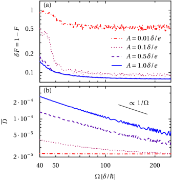
Figure 3: (Color online) (a) Fidelity defect $\delta F=1-F$ and (b) time-averaged trace distance $\overline{D}$ between the density operators of a driven and an undriven CPB during a LZ sweep. Both quantities are depicted for various driving amplitudes $A$ as a function of the driving frequency $\Omega$. All other parameters are the same as in Fig. 2.

The measurement fidelity defect $\delta F=1-F$ between $\phi_{\mathrm{out}}^{\text{exp}}(t)$ and $\phi^{0}_{\text{hf}}(t)$, computed with Eq. (25), is depicted in Fig. 3(a) as a function of the driving frequency. Apparently, resonant excitations to non-qubit CPB states play a minor role here since, in contrast to the case of a time-independent qubit energy, Reuther et al. (2009) we do not observe characteristic resonance peaks in $\delta F$. Since all CPB frequencies are varied in time during the LZ sweep, the population of non-qubit states by the driving is mainly suppressed. Furthermore, the fidelity only slightly increases after the driving frequency $\Omega$ has exceeded a minimal value of $v\tau_{\mathrm{LZ}}/\hbar$. This corroborates that $\Omega\approx 50\delta/\hbar$ is a good choice.

With regard to the driving amplitude, one has to find a compromise. The phase contrast of the outgoing signal (21) obviously increases with $A$, whereas the driving perturbs more and more the low-frequency dynamics. Here, the choice of $A=\delta/e$ yields a maximum fidelity of $F\simeq 0.9$ for the above driving frequency. This apparently low value essentially stems from the discussed deviation between $\phi_{\text{out}}^{\text{exp}}(t)$ and $\phi^{0}_{\text{hf}}(t)$. Far from a subsequent LZ sweep, the system is faithfully described with only the qubit levels. All in all, for these values, $eA/\hbar\Omega\approx 0.01$–$0.1$, which justifies our perturbative treatment.

The small-dissipation condition $\alpha\lesssim 0.1$ together with the above conditions on the driving amplitude and frequency provides phase shifts of roughly $\phi_{\mathrm{out}}^{\text{exp}}\approx 0.1^{\circ}$, which is small but still measurable with present technologies. In particular, the constraint of large driving frequencies $\Omega$ for monitoring a LZ sweep reduces the maximum visibility of the oscillations encoded in the phase shift. In contrast, a smaller value of $\Omega$, if applicable, may result in a visibility of the order of $1^{\circ}$. We turn back to these quantitative issues in Sec. V where we discuss the collective dynamics of equal quantum systems.

Generally, decoherence may be influenced by ac driving. Kohler et al. (1997) Here, however, we do not observe a significant change of decoherence. We conclude this from Fig. 3(b) which depicts the time-averaged trace distance, computed with Eq. (27) as a function of the driving frequency for various driving amplitudes. For intermediate amplitudes, we find roughly $\overline{D}\propto A/\Omega$, unless $A$ is very small, which agrees with relation (26). This states that at high frequencies, the driving does not add decoherence, which confirms the picture drawn by investigating the measurement fidelity $F$.

Our model Hamiltonian does not consider the excitation of quasi-particles in the superconductor. Therefore it is valid only as long as the driving frequency stays below the gap energy. Thus, a setup made of aluminum the driving is limited to $\Omega\lesssim 100\,\mathrm{GHz}$. With a typical Josephson energy of the order of some GHz, the driving frequency required to monitor the dynamics of a LZ sweep already comes close to this limit. An implementation with niobium, whose energy gap is considerably larger Novotny and Meincke (1975) and which has been used in circuit QED experiments, Berns et al. (2008) should be less critical.

IV Two-qubit entanglement

When considering a second qubit, it may be entangled with the first one. In the present context, this raises the question whether our measurement scheme is sensitive to this property. In order to dwell into this question, we focus on a system of two charge qubits described by the Hamiltonian

$$H_{\mathrm{2q,0}}=\frac{\omega}{2}(\sigma_{z}^{(1)}+\sigma_{z}^{(2)})+g\sigma_{x}^{(1)}\sigma_{x}^{(2)},$$ (33)

where the upper indices label the qubits. Here, we assume that both qubits possess the same energy splitting $\omega$ and are mutually coupled with strength $g$. A qubit coupling scheme as described here is effectively realized in the case of, e.g., two CPBs within two-level approximation which are capacitively coupled to a transmission line resonator. In analogy to the above discussions, our measurement scheme can be applied on condition that the driving field is not in resonance with transitions to higher energy levels of the underlying physical system. Reuther et al. (2009) If the qubit-resonator interaction is dispersive, i.e., if the resonator is far detuned with respect to the qubits, it mediates an effective qubit-qubit $XX$-coupling, Zueco et al. (2009) such that the two-qubit system can be described by the effective Hamiltonian (33). Alternatively, an effective $XX$-coupling between two qubits can be mediated by a third, dispersively detuned qubit. Niskanen et al. (2007)

Both charge qubits couple capacitively to a common environment via their charge operator

$$Q_{\mathrm{2q}}=e(\sigma_{z}^{(1)}+\sigma_{z}^{(2)})\,.$$ (34)

An adequate measurement of the qubit-qubit entanglement is the concurrence

$$C=\max\{\chi_{1}-\chi_{2}-\chi_{3}-\chi_{4},0\}\;,$$ (35)

where the $\chi_{j}$ denote the ordered square roots of the eigenvalues of the matrix $\rho(\sigma_{y}^{(1)}\sigma_{y}^{(2)})\rho^{*}(\sigma_{y}^{(1)}\sigma_{y}^{(2)})$ with $\rho$ denoting the two-qubit density matrix. Wootters (1998)

For later convenience we express the system operators in terms of the four, maximally entangled Bell states,

$$|\Phi_{\pm}\rangle =\frac{1}{\sqrt{2}}\left(|00\rangle\pm|11\rangle\right)\;,$$ (36)

$$|\Psi_{\pm}\rangle =\frac{1}{\sqrt{2}}\left(|10\rangle\pm|01\rangle\right)\,.$$ (37)

In the basis $\{|\Phi_{+}\rangle,|\Phi_{-}\rangle,|\Psi_{+}\rangle,|\Psi_{-}\rangle\}$ the two-qubit Hamiltonian (33) reads

$$H_{\mathrm{2q,0}}=\frac{1}{2}\begin{pmatrix}\hphantom{-}g&-\omega&\,0&0\\ -\omega&-g&\,0&0\\[2.15277pt] 0&0&\,g&0\\ 0&0&\,0&-g\end{pmatrix},$$ (38)

while the charge operator becomes

$$Q_{\mathrm{2q}}=2e\begin{pmatrix}0&1&0&0\\ 1&0&0&0\\ 0&0&0&0\\ 0&0&0&0\end{pmatrix}.$$ (39)

This representation of the coupling to the environment evidences that neither the system-bath coupling nor the ac driving generate transitions between the subspaces spanned by the states $\{|\Phi_{\pm}\rangle\}$ and $\{|\Psi_{\pm}\rangle\}$, respectively. Concerning the latter states, it is even such that they are not coupled to the environment at all, i.e., they form a decoherence-free subspace. Lidar et al. (1998); Yu and Eberly (2002) For this reason, we henceforth focus on initial preparations in the subspace spanned by $\{|\Phi_{\pm}\rangle\}$. In this particular case, the concurrence is given by

$$C_{\{|\Phi_{\pm}\rangle\}}(t)=2|\rho_{0011}(t)|\equiv 2|\mathrm{Tr}\{\rho(t)|00\rangle\langle 11|\}|,$$ (40)

i.e., by an off-diagonal density matrix element in the product basis. In terms of the pseudo-spin operators $\sigma_{z}^{\prime}$ and $\sigma_{x}^{\prime}$ defined in the basis $\{|\Phi_{+}\rangle,|\Phi_{-}\rangle\}$, the Hamiltonian and the charge operator become

$$H_{\mathrm{2q,0}}^{\prime} =g\sigma_{z}^{\prime}-\omega\sigma_{x}^{\prime}\;,$$ (41)

$$Q_{\mathrm{2q}}^{\prime} =2e\sigma_{x}^{\prime}\;,$$ (42)

respectively.

At this point, we recall Eq. (24) which relates the phase of the outgoing signal to a particular observable of the undriven system. Inserting the subspace Hamiltonian and charge operator, Eqs. (41) and (42), we obtain

$$\phi_{\mathrm{hf}}^{0}(t)=\frac{32g\alpha}{\hbar\Omega}\left\langle\sigma_{z}^{\prime}\right\rangle_{0,t}\;,$$ (43)

with the dimensionless damping strength $\alpha=e^{2}Z_{0}/\hbar$, and

$$\langle\sigma_{z}^{\prime}\rangle_{0,t}\equiv\mathrm{Tr}\{\rho_{0}(t)\sigma_{z}^{\prime}\}=2\mathrm{Re}\{\rho_{0011}^{0}(t)\}\,.$$ (44)

In other words, the phase of the outgoing signal is proportional to the real part of the density matrix element $\rho_{0011}^{0}(t)$ of the unperturbed system. Figure 4 demonstrates that this relation holds sufficiently well: It compares the numerically calculated phase of the lock-in measurement, $\phi_{\mathrm{out}}^{\text{exp}}(t)$, to the phase $\phi_{\mathrm{hf}}^{0}(t)\propto\langle\sigma_{z}^{\prime}\rangle_{0,t}$ predicted by the measurement relation (24). We find an excellent agreement between both quantities, while the maximum angular visibility reaches values of around $1^{\circ}$. Thus, we find that it is possible to access directly the key density matrix element needed to reconstruct the concurrence $C_{\{|\Phi_{\pm}\rangle\}}(t)$ for the subspace $\{|\Phi_{\pm}\rangle\}$.

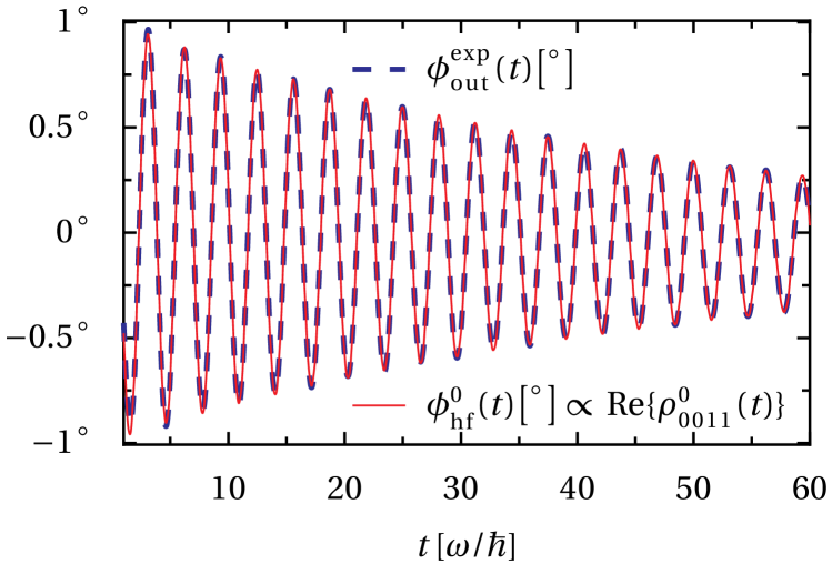
Figure 4: (Color online) Monitoring the entanglement evolution of two coupled qubits with initial state ${|}\Phi_{+}\rangle$. The lock-in amplified phase $\phi_{\text{out}}^{\text{exp}}$ (blue dashed line) is compared to the estimated phase $\phi_{\mathrm{hf}}^{0}(t)$ (red solid line) which is proportional to the real part of the density matrix element $\rho^{0}_{0011}(t)$. The latter is needed for reconstructing the concurrence $C(t)=2|\rho^{0}_{0011}(t)|$ of the unperturbed system. Parameters are $\Omega=15\,\omega$, $g=0.1\,\omega$, $A=0.1\,\omega$ and $\alpha=0.08$.

Monitoring $\mathrm{Re}\{\rho_{0011}^{0}(t)\}$ already provides a lower bound for the entanglement and may even provide a good estimate for it. Nevertheless, it is desirable to measure also its imaginary part. For this purpose one has to rotate the basis of the second qubit by applying the phase gate

$$U_{\mathrm{phase}}^{(2)}=\begin{pmatrix}1&0\\ 0&i\end{pmatrix}.$$ (45)

This local unitary transform does not alter the two-qubit entanglement at the time it is applied. For small values of $g$, it approximately commutes with the total time evolution operator of the system, $\exp(iHt/\hbar)$. i.e., $[\exp(iHt/\hbar),U_{\mathrm{phase}}^{(2)}]=0$ for $g=0$. In analogy to Eq. (44), the relation for the phase shift then becomes

$$\phi_{\mathrm{hf}}^{0}(t)\propto\mathrm{Im}\{\rho_{0011}^{0}(t)\}\,.$$ (46)

Thus, we have access to both the real and the imaginary part of the density matrix element $\rho_{0011}^{0}(t)$. One just needs to initiate two copies of a pure entangled state in the subspace $\{|\Phi_{\pm}\rangle\}$, apply the gate of Eq. (45) to one of them, and monitor their dissipative time evolution. The difference between the two-qubit dynamics in either case due to the phase gate $U_{\mathrm{phase}}^{(2)}$ is relevant only at large times when the qubits approach their stationary state. For the transient stage depicted in Fig. 4, we have verified that the phase of the output signal indeed reflects the imaginary part of the concurrence (not shown). This, in turn, enables one to reconstruct the characteristics of the concurrence $C_{\{|\Phi_{\pm}\rangle\}}(t)$ and thus of the amount of entanglement between the two qubits, according to Eq. (40).

In a similar way, one finds access to the entanglement when the system is initially prepared in the subspace $|\Psi_{\pm}\rangle$. This can be done by applying the so-called Pauli-X gate to the second qubit,

$$U_{\mathrm{X}}^{(2)}\equiv\sigma_{x}^{(2)}=\begin{pmatrix}0&1\\ 1&0\end{pmatrix}\;,$$ (47)

effectively leaving us in the $|\Phi_{\pm}\rangle$ subspace again, from where one can pursue as described above. Like this, it is possible to monitor the time characteristics of entanglement of all kinds of entangled two-qubit states, as long as the subspaces $\{|\Phi_{\pm}\rangle\}$ and $\{|\Psi_{\pm}\rangle\}$ are not mixed.

Admittedly, the relation between the entanglement and $\phi_{\text{hf}}^{0}$, manifest in Eqs. (43) and (44), holds only if the concurrence can be expressed as the expectation value of an observable providing the required off-diagonal matrix element of the density operator. Obviously, this does not always apply. However, two qubits prepared in a Bell state represent such a case which is of relevance and interest.

So far, we have addressed initially pure entangled states, which constitutes an idealization and is not always achievable in an experiment. A more realistic scenario copes with the drawback that one starts from a mixed state which naturally possesses less entanglement. Moreover, the concurrence is then no longer determined by a single off-diagonal matrix element [cf. Eq. (40)], but rather has to be computed from the definition of the two-qubit concurrence, Eq. (35). In order to test how much information about the concurrence $C(t)$ is nevertheless contained in the measurement signal (43), we study the time evolution for the preparation in an unpolarized mixture or Werner state, Werner (1989)

$$\rho_{\mathrm{W}}=(1-p)|\Phi_{+}\rangle\langle\Phi_{+}|\\ +\frac{p}{3}\left(|\Phi_{-}\rangle\langle\Phi_{-}|+|\Psi_{+}\rangle\langle\Psi_{+}|+|\Psi_{-}\rangle\langle\Psi_{-}|\right)\;,$$ (48)

where $p$ denotes the degree of depolarization. A perfect initial preparation in the fully entangled state $|\Phi_{+}\rangle$ is then characterized by $p=0$. For $p>0.5$, the state is separable. In the realm of circuit QED, a polarization degree of $p=0.1$ has already been achieved, Ansmann et al. (2009) while in a quantum optical context, even the much lower value $p\lesssim 0.01$ could be reached. Lougovski et al. (2005)

Our goal is now to compare the concurrence $C(t)$ with $C_{\{|\Phi_{\pm}\rangle\}}(t)$ which holds for preparation in a Bell state. As a measure for the agreement, we use again the fidelity $F$ defined as the scaled overlap between both quantities, i.e., by Eq. (25) but with the phases replaced by the concurrences. Figure 5 shows the resulting fidelity defect $\delta F=1-F$ as a function of the initial degree of depolarization. From a numerical comparison of the concurrence curves $C(t)$ and $C_{\{|\Phi_{\pm}\rangle\}}(t)$ for different values of $\delta F$ (not shown), we set the threshold for the maximum acceptable fidelity defect to $\delta F_{\mathrm{max}}=0.03$. The investigation of several examples showed that, beyond a fidelity defect of this order, both curves no longer appear similar. Thus, it appears that the measured phase shift captures the concurrence dynamics satisfactorily only for a $\delta F$ below this threshold. Remarkably, the latter is not reached until an initial depolarization of $p\lesssim 0.1$. From this, we conclude that our measurement protocol allows one to gain information about qubit-qubit entanglement in circuit QED even for depolarized initial states.

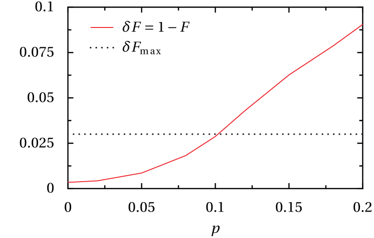
Figure 5: (Color online) Fidelity defect $\delta F=1-F$ of the concurrence curves $C_{\{|\Phi_{\pm}\rangle\}}(t)$ and $C(t)$ in dependence of the degree of depolarization, $p$. The function overlap is integrated over the decay time of the two-qubit state. As discussed in the text, the upper bound $\delta F_{\mathrm{max}}=0.03$ marks the largest acceptable value of $p$. All other parameters as in Fig. 4.

V Collective quantum dynamics

The typical signal that can be reached with our protocol, as regards measurements of single quantum systems, is a phase shift of the order $1^{\circ}$, as estimated in Sec. III. Of practical interest is whether this already marks the maximum reachable. In the following, we suggest how to increase the visibility by monitoring the collective dynamics of a large number of identical quantum objects at the same time. For this purpose, we exemplarily investigate an “atomic cloud” containing a large number of atoms as described in Ref. Verdú et al., 2009. There, an ensemble of cold atoms interacting with a superconducting cavity, described by the Dicke model, was investigated. Provided that it is possible to single out one particular atomic transition, the cloud represents an ensemble of identical two level atoms. This gives rise to the $N$-qubit Hamiltonian

$$H_{N\mathrm{q},0}=\epsilon\sum_{j=1}^{N}\sigma_{z}^{(j)}+\delta\sum_{j=1}^{N}\sigma_{x}^{(j)}\,.$$ (49)

The interaction between the electromagnetic field in the cavity and the atoms is assumed dipole-like and can be cast into the operator $Q_{N\mathrm{q}}(a+a^{\dagger})$. Here, the collective coupling operator $Q_{N\mathrm{q}}$ is chosen dimensionless and given as

$$Q_{N\mathrm{q}}=\sum_{j=1}^{N}\sigma_{z}^{(j)}=\sqrt{N}S_{z}\,,$$ (50)

and $S_{z}=\sum_{j=1}^{N}\sigma_{z}^{(j)}/\sqrt{N}$ denotes the collective spin of the cloud.

In the case where an open transmission line is employed in the setup rather than the (closed) cavity, a continuum of modes replaces the single cavity mode in the modeling. In this sense, the transmission line can be understood as one-dimensional heat bath. The dipole interaction between the cloud and the environment becomes $H_{\mathrm{int}}=Q_{N\mathrm{q}}\sum_{k}c_{k}(a_{k}^{\dagger}+a_{k}^{\vphantom{\dagger}})$. Thus, one naturally ends up with the Caldeira-Legget model of Eq. (1) where, formally, $c_{k}=\lambda_{k}\omega_{k}/C_{k}$.

Assuming an ohmic environment, the phase shift (24) then becomes

$$\phi_{\mathrm{hf}}^{0}(t)=\frac{2\alpha}{\hbar\Omega}\left\langle[[H_{0},Q],Q]\right\rangle_{0,t}\;,$$ (51)

where $\alpha$ denotes the dimensionless damping strength, and $\alpha\delta$ is the coupling strength to the environment per atom. Inserting $H_{N\mathrm{q},0}$ and $Q_{N\mathrm{q}}$ into the measurement relation (51) yields

$$\phi_{\mathrm{hf}}^{0}(t)=\frac{4\alpha\delta\sqrt{N}}{\hbar\Omega}\left\langle S_{x}\right\rangle_{0,t}$$ (52)

with $S_{x}=\sum_{j=1}^{N}\sigma_{x}^{(j)}/\sqrt{N}$. Thus, the phase signal scales with $\sqrt{N}$ as compared to Eq. (29). By virtue of this relation, monitoring the collective dynamics of $N$ two-level systems via the total spin paves the way towards a higher angular visibility.

Since the validity of the measurement relation (51) is restricted to small angles, the visibility may be enhanced up to the order $10^{\circ}$. In order to be specific, we evaluate $\phi_{\text{hf}}^{0}$ for the parameters Verdú et al. (2009) $\delta/2\pi\hbar=6.8\mathrm{GHz}$, $\alpha=6\cdot 10^{-5}$, $\Omega/2\pi=20\mathrm{GHz}$. This yields an effective single-atom coupling to the ohmic environment of $\alpha\delta/2\pi\hbar\approx 0.4\mathrm{MHz}$. Despite this very small system-bath interaction strength per atom, the estimated phase resolution for $N=10^{6}$ atoms in the cloud reaches $\phi_{\mathrm{hf}}^{0}=4^{\circ}-5^{\circ}$. At the same time, atomic decoherence is drastically reduced. Under these conditions, which are experimentally achievable,Verdú et al. (2009) the real-time monitoring of an atomic ensemble constitutes a major improvement in angular visibility in comparison with the single-qubit case.

VI Conclusions

We have derived a scheme for monitoring the low-frequency dynamics of a quantum system, where a particular focus has been put on quantum circuits. The central idea is to couple the quantum system capacitively to a high-frequency ac field and to measure the reflected signal. We have shown that the phase of the latter contains information about a particular expectation value of the central system. In an experiment, this information can be extracted with lock-in techniques. This scheme has some similarities to the qubit readout via a tank circuit Grajcar et al. (2004); Sillanpää et al. (2005) or a quantum point contact. Ashhab et al. (2009) The essential difference is that the proposed high-frequency driving enables a time-resolved measurement.

The underlying relation (24) between a particular expectation value and the phase shift of the reflected signal relies on a time-scale separation. This constitutes an approximation, which has to be validated. In so doing, we have demonstrated that the measurement fidelity is rather good. As an example, we have studied a qubit undergoing Landau-Zener transitions. Owing to the time dependent level splitting of the qubit, its dynamics possesses a broad frequency spectrum. Thus, it represents a more challenging test case than the coherent oscillations considered in Ref. Reuther et al., 2009. Also for the present case, the measurement fidelity turned out to be rather good.

A further relevant issue is the backaction of the measurement on the system. The relevant backaction is decoherence which here is unavoidable because the driving and the environmental degrees of freedom couple to the system via the same mechanism. This is reflected by the fact that the phase shift being the recorded signal is proportional to the decoherence rate. Thus a stronger coupling to the driving can be achieved only at the expense of more decoherence.

Concerning possible applications in solid-state quantum information processing, the generalization towards systems with two or more qubits is rather important. For the case of two qubits, we have demonstrated that it is possible to monitor the time evolution of their entanglement, provided that one can access the relevant density matrix elements via the phase shift of the reflected signal. Even though the entanglement decays due to the unavoidable decoherence, it is still possible to monitor an appreciable number of cycles between entangled and separable states of interacting qubits. Furthermore, our protocol produces reliable results even in the case where the monitored state is mixed rather than pure.

Finally, we have also addressed the question of how much stronger the measurement signal can be if the single qubit is replaced by a whole array of qubits that undergo the same dynamics. The result is that the signal scales with the square root of the number of qubits. This even leaves some room for improving the fidelity and reducing the coupling to each qubit. As a consequence, decoherence becomes less relevant, which is encouraging in particular when attempting a proof-of-principle realization.