An unified timing and spectral model for the Anomalous X-ray Pulsars
XTE J1810-197 and CXOU J164710.2-455216

Abstract

Anomalous X-ray pulsars (AXPs) and soft gamma repeaters (SGRs) are two small classes of X-ray sources strongly suspected to host a magnetar, i.e. an ultra-magnetized neutron star with $B\approx 10^{14}$–$10^{15}$ G. Many SGRs/AXPs are known to be variable, and recently the existence of genuinely “transient” magnetars was discovered. Here we present a comprehensive study of the pulse profile and spectral evolution of the two transient AXPs (TAXPs) XTE J1810-197 and CXOU J164710.2-455216. Our analysis was carried out in the framework of the twisted magnetosphere model for magnetar emission. Starting from 3D Monte Carlo simulations of the emerging spectrum, we produced a large database of synthetic pulse profiles which was fitted to observed lightcurves in different spectral bands and at different epochs. This allowed us to derive the physical parameters of the model and their evolution with time, together with the geometry of the two sources, i.e. the inclination of the line-of-sight and of the magnetic axis with respect to the rotation axis. We then fitted the (phase-averaged) spectra of the two TAXPs at different epochs using a model similar to that used to calculate the pulse profiles (ntzang in XSPEC) freezing all parameters to the values obtained from the timing analysis, and leaving only the normalization free to vary. This provided acceptable fits to XMM-Newton data in all the observations we analyzed. Our results support a picture in which a limited portion of the star surface close to one of the magnetic poles is heated at the outburst onset. The subsequent evolution is driven both by the cooling/varying size of the heated cap and by a progressive untwisting of the magnetosphere.

1. Introduction

In recent years an increasing number of high-resolution spectral and timing observations of isolated neutron stars has become available. Many of these observations concern two peculiar classes of high-energy pulsars, the Anomalous X-Ray Pulsars (AXPs: 9 objects plus 1 candidate) and the Soft Gamma-Ray Repeaters (SGRs: 6 objects) . Historically these two classes of sources were regarded as distinct. While SGRs were first discovered in late 1978-early 1979, when SGR 1806-20 and SGR 0526-66 exhibited a bright burst of soft $\gamma$-rays (Mazets et al., 1979; Laros et al., 1986), AXPs were observed for the first time in 1981, when Fahlman, & Gregory (1981) discovered pulsations in the EINSTEIN source 1E 2259+586. It was, however, not until the mid ’90s that AXPs were recognized as a class of “anomalous” pulsars because of their luminosity substantially exceeding rotational energy losses (Mereghetti, & Stella, 1995).

Although SGRs were mainly known as emitters of short, energetic bursts, they are also persistent X-ray sources with properties quite similar to those of AXPs (see e.g. Woods & Thompson, 2006; Mereghetti, 2008, for reviews). They all are slow X-ray pulsars, with spin periods in a very narrow range ($P\sim 2$–12 s), relatively large spin-down rates ($\dot{P}\sim 10^{-13}$–$10^{-11}\ {\rm s\ s}^{-1}$), spin down ages of $10^{3}$–1$0^{4}\ {\rm yr}$, and stronger magnetic fields compared to those of rotation or accretion powered pulsars ($B\sim 10^{14}$–$10^{15}\ {\rm G}>B_{QED}\simeq 4.4\times 10^{13}\ {\rm G}$). AXPs and SGRs have persistent X-ray luminosities $L_{X}\sim 10^{34}$–$10^{36}\ {\rm erg\ s}^{-1}$. Their spectra in the 0.1–10 keV band are relatively soft and can be empirically fitted with a two-component model, an absorbed blackbody ($kT\sim 0.2$–0.6 keV) plus a power-law ($\Gamma\sim 2$–4). INTEGRAL observations revealed the presence of sizeable emission up to $\sim 200$ keV, which accounts for up to $50\%$ of the total flux. Hard X-ray spectra are well represented by a power-law, which dominates above $\sim 20$ keV in AXPs.

The large high-energy output can not be explained in terms of rotational energy losses, as in conventional models for radio-pulsars, while the lack of stellar companions argues against accretion. The powering mechanism of AXPs and SGRs, instead, is believed to reside in the neutron star ultra-strong magnetic field (magnetar; Duncan, & Thompson 1992, Thompson & Duncan 1993). The magnetar scenario appears capable to explain the properties of both the bursts (Thompson & Duncan, 1995) and the persistent emission (the twisted magnetosphere model, Thompson, Lyutikov, & Kulkarni, 2002; Zane et al., 2009, and references therein; see § 3 for details), although no definite model for the hard tails was put forward as yet.

The persistent emission of SGRs and AXPs is now known to be variable. AXPs, in particular, display different types of X-ray flux variability: from slow, moderate flux changes on timescales of months/years, to intense outbursts with short rise times ($\sim 1$ day) lasting $\sim 1$ year. Some AXPs were found to undergo intense and dramatic SGR-like burst activity on sub-second timescales (XTE J1810-197, 4U 0142+614, 1E 1048.1-5973, CXOU J164710.2-455216 and 1E 2259+586). The discovery of bursts from AXPs is regarded as further evidence in favor of a common nature of AXPs and SGRs.

The first case of AXP flux variability was observed in 2002, when 1E 2259+586 showed an increase in the persistent flux by a factor $\sim 10$ with respect to the quiescent level, followed by the emission of $\sim 80$ short bursts with luminosity $L_{X}\sim 10^{36}-10^{38}\ {\rm erg\ s}^{-1}$ (Kaspi et al., 2003). In early 2003 the 5.54 s AXP XTE J1810-197 was discovered at a luminosity $\sim 100$ greater than its quiescent value ($10^{33}\ {\rm erg\ s}^{-1}$; Ibrahim et al., 2004). Analysis of archival data revealed that the outburst started between November 2002 and January 2003.

On September 21st 2006 an outburst was observed from the AXP CXOU J164710.2-455216 ($P=10.61$ s). The flux level was $\sim 300$ times higher than that measured only 5 days earlier by XMM-Newton (Muno et al., 2006b; Campana, & Israel, 2006; Israel, & Campana, 2006). This, much as in the case of XTE J1810-197, indicates that some AXPs are transient sources (dubbed Transient AXPs) and may become visible only when they enter an active state. Recently other AXPs and SGRs showed a series of short bursts of soft $\gamma$-rays which was detected by different satellites (Mereghetti et al., 2009).

In this paper we present a comprehensive study of the pulse profile and spectral evolution of the TAXPs XTE J1810-197 and CXOU J164710.2-455216 throughout their outbursts of November 2002 and September 2006, respectively. By confronting timing data with synthetic lightcurves obtained from the twisted magnetosphere model (Nobili, Turolla, & Zane, 2008), we were able to estimate how the physical parameters of the source (surface temperature and emitting area, electron energy, twist angle) evolve in time. The fits of the pulse profiles also allowed us to infer the geometry of the two systems, i.e. the angles between the magnetic and rotational axes and the line of sight. Spectral models, obtained with the parameter values derived from the timing analysis, provide acceptable fits to XMM-Newton data.

2. Transient AXPs properties

2.1. XTE J1810-107

The Transient AXP (TAXP) XTE J1810-197 was serendipitously discovered in 2003 with the Rossi X-Ray Timing Explorer (RXTE) while observing SGR 1806-20 (Ibrahim et al. 2004). The source was readily identified as a X-ray pulsar, and soon after a search in archival RXTE data showed that it produced an outburst around 2002 November, followed by a monotonic decline of the X-ray flux. The X-ray pulsar spin period was found to be 5.54 s, with a spin-down rate $\sim 10^{-11}\ {\rm s\ s}^{-1}$. Using the standard expression for magneto-rotational losses, the inferred value of the (dipolar) magnetic field is $B\sim 3\times 10^{14}\ {\rm G}$ (Ibrahim et al., 2004). The source was classified as the first transient magnetar. The TAXP XTE J1810-197 was then studied with Chandra and XMM-Newton Gotthelf et al. (2004); Israel et al. (2004); Gotthelf, & Halpern (2005, 2007), in order to monitor its evolution in the post-outburst phase.

By using archival Very Large Array (VLA) data a transient radio emission with a flux of $\sim 4.5\ {\rm mJy}$ at $1.4\ {\rm GHz}$ was discovered at the Chandra X-ray position of XTE J1810-197 (Halpern et al., 2005). Only later on it was discovered that this radio emission was pulsed, highly polarized and with large flux variability even on very short timescales (Camilo et al. 2006). The X-ray and the radio pulsations are at the same rotational phase. Since accretion is expected to quench radio emission, this is further evidence against the source being accretion-powered.

Deep IR observations were performed for this source, revealing a weak ($K_{s}=20.8$ mag) counterpart, with characteristics similar to those of other AXPs (Israel et al., 2004). The IR emission is variable (Rea et al., 2004), but no correlations between the IR and X-ray changes were found up to now. The existence of a correlation at IR/radio wavelengths is uncertain (Camilo et al., 2006, 2007; Testa et al., 2008).

XTE J1810-197 was observed 9 times by XMM-Newton, between September 2003 and September 2007, two times every year. The uninterrupted coverage of the source during 4 years provides an unique opportunity to understand the phenomenology of TAXPs. Earlier observations of XTE J1810-197 showed that the source spectrum is well reproduced by a two blackbody model, likely indicating that (thermal) emission occurs in two regions of the star surface of different size and temperature: a hot one ($kT=0.70\ {\rm keV}$) and a warm one ($kT=0.30\ {\rm keV}$; Gotthelf, & Halpern 2005). XMM-Newton observations also showed that the pulsed fraction decreases in time.

Perna & Gotthelf (2008) discussed the post-outburst spectral evolution of XTE J1810-197 from 2003 to 2005 in terms of two blackbody components, one arising from a hot spot and the other from a warm concentric ring. By varying the area and temperature of the two regions, this (geometric) model can reproduce the observed spectra, account for the decline of the pulsed fraction with time and place a strong constrain on the geometry of the source, i.e. the angles between the line of sight and the hot spot axis with respect to the spin axis.

Recently, Bernardini et al. (2009) by re-examining all available XMM-Newton data found that inclusion of a third spectral component, a blackbody at $\sim 0.15$ keV, improved the fits. When this component is added both the area and temperature of the hot component was found to monotonically decrease in time, while the warm component decreased in area but stayed at constant temperature. The coolest blackbody, which appeared not to change in time, is associated to emission from the (large) part of the surface which was not affected by the event which triggered the outburst, and is consistent with the spectral properties of the source as derived from a ROSAT detection before the outburst onset. Finally, an interpretation of XTE J1810-197 spectra in terms of a resonant compton scattering model (RCS, see §3) was presented by Rea et al. (2008).

2.2. CXOU J164710.2-455216

The TAXP CXOU J164710.2-455216 was discovered in two Chandra pointings of the young Galactic star cluster Westerlund 1 in May/June 2005. The period of the X-ray pulsar was found to be $P=10.61$ s (Muno et al., 2006), with a period derivative $\dot{P}=9\times 10^{-13}\ {\rm s\ s}^{-1}$ (Israel et al., 2007). The implied magnetic field is $B\sim 10^{14}\ {\rm G}$.

In November 2006, an intense burst was detected by the Swift Burst Alert Telescope (BAT) in Westerlund 1 (Krimm et al., 2006; Muno et al., 2006). Its short duration ($20\ {\rm ms}$) suggested that its origin was the candidate AXP. However the event was initially attributed to a nearby Galactic source, so the AXP was not promptly re-observed by Swift. A ToO observation program with Swift was started 13 hrs after the burst, displaying a persistent flux level $300$ times higher than the quiescent one. CXOU J164710.2-455216 was observed in radio, with the Parkes Telescope. The observation was carried out a week after the outburst onset, with the intent of searching for pulsed emission similar to that of XTE J1810. In this case, however, only a (tight) upper limit to the radio flux ($40\ \mu{\rm Jy}$) was placed (Burgay et al., 2006).

XMM-Newton observations carried out across the outburst onset show a complex pulse profile evolution. Just before the event the pulsed fraction was $\sim 65\%$, while soon after it became $\sim 11\%$ (Muno et al., 2007). Moreover, the pulse profile changed from being single-peaked just before the burst, to showing three peaks soon after it. CXOU J164710.2-455216 spectra in the outburst state were fitted either with a two blackbody model ($kT_{1}\sim 0.7\ {\rm keV}$, $kT_{2}\sim 1.7\ {\rm keV}$), or with a blackbody plus power-law model ($kT\sim 0.65\ {\rm keV}$, $\Gamma\sim 2.3$; Muno et al., 2007; Israel et al., 2007). Rea et al. (2008) found that a RCS model also provides a good fit to the data.

3. The model

It is now widely accepted that AXPs and SGRs are magnetars, and that their burst/outburst activity, together with the persistent emission, are powered by their huge magnetic field. In particular, the soft X-ray spectrum ($\sim 1$–10 keV) is believed to originate in a “twisted” magnetosphere ($\nabla\times{\mathbf{B}}\neq 0$; Thompson, Lyutikov, & Kulkarni, 2002), where the currents needed to support the field provide a large enough optical depth to resonant Compton scattering of thermal photons emitted by the star surface. Since charges are expected to flow along the closed field lines at relativistic velocities, photons gain energy in the (resonant) scatterings and ultimately fill a hard tail.

Most studies on spectral formation in a twisted magnetosphere (Lyutikov, & Gavriil, 2006; Fernandez, & Thompson, 2007; Nobili, Turolla, & Zane, 2008) are based on the axially symmetric, force-free solution for a twisted dipolar field presented by Thompson, Lyutikov, & Kulkarni (2002). This corresponds to a sequence of magnetostatic equilibria which, once the polar strength of the magnetic field $B_{p}$ is fixed, depends only on a single parameter: the radial index of the magnetic field $p$ ($B\propto r^{-p-2}$, $0\leq p\leq 1$) or, equivalently, the twist angle

$$\Delta\phi_{N-S}=\lim_{\theta_{0}\to 0}2\int_{\theta_{0}}^{\pi/2}\frac{B_{\phi}}{B_{\theta}}\frac{d\theta}{\sin\theta}\,,$$ (1)

where $B_{r},B_{\theta}$ and $B_{\phi}$ are the spherical components of the field, which depend only on $r$ and $\theta$ because of axial symmetry. Knowledge of ${\mathbf{B}}$ fixes the current density ${\mathbf{j}}=(c/4\pi)\nabla\times{\mathbf{B}}$, and, if the particle velocity is known, also the electron density in the magnetosphere

$$n_{e}(r,\theta)=\frac{p+1}{4\pi e}\Bigl{(}\frac{B_{\phi}}{B_{\theta}}\Bigr{)}\frac{B}{r|\langle\beta\rangle|}$$ (2)

where $e$ is the electron charge and $\langle\beta\rangle$ is the average charge velocity (in units of $c$). The charge density of the space charge-limited flow of ions and electrons moving along the closed field lines is orders of magnitude larger than the Goldreich-Julian density, $n_{GJ}$, associated to the charge flow along the open field lines in radio-pulsars.

In our investigation we make use of the spectral models presented by Nobili, Turolla, & Zane (2008, NTZ in the folowing), who studied radiative transfer in a globally twisted magnetosphere by means of a 3D Monte Carlo code. Each model is characterized by the magnetospheric twist $\Delta\phi_{N-S}$, the electron (constant) bulk velocity $\beta$, and the seed photon temperature $kT$. The polar field was fixed at $B_{p}=10^{14}\ {\rm G}$. In the applications presented by NTZ, it was assumed that the star surface emits unpolarized, blackbody radiation and is at uniform temperature. Concerning the present investigation, the most critical assumption is that of a globally twisted magnetosphere, as discussed in some more detail in § 5. Taking a constant value for the electrons bulk velocity is certainly an oversimplification and reflects the lack of a detailed model for the magnetospheric currents. In a realistic case one would expect that $\beta$ is a function of position. However, resonant scattering is possible only where the bulk velocity is mildly relativistic. If along a flux tube there are large variations of the Lorentz factor, only the region where $\beta\approx 0.5$ will contribute to scattering. Moreover, preliminary calculations of the dynamics of charged particles in a twisted force-free magnetosphere performed accounting for both electrostatic acceleration and Compton drag indicate that $\beta$ is indeed fairly constant along the central part of a flux tube (Beloborodov, private communication). The assumption of unpolarized thermal radiation is not cogent either, since we are not interested in the polarization of the escaping radiation and the emergent spectrum is quite insensitive to the polarization fraction of the seed photons (see, e.g., Fig. 4 of NTZ).

The code works by dividing the stellar surface into $N_{\Theta}\times N_{\Phi}$ zones of equal area by means of a ($\cos\Theta$, $\Phi$) grid, where $\Theta$ is the magnetic colatitude and $\Phi$ the longitude. After a few scatterings photons escape from the neutron star magnetosphere and are collected on a spherical surface (the “sky”) which is divided into $N_{\Theta_{s}}\times N_{\Phi_{s}}$ patches, similarly to what is done for the star surface. The key point is that the evolution of seed photons from each patch is followed separately. This allows us to treat an arbitrary surface temperature distribution without the need to perform new Monte Carlo runs, by simply combining together models from runs with different temperatures at the post-production level (the geometry is shown in Fig. 1)

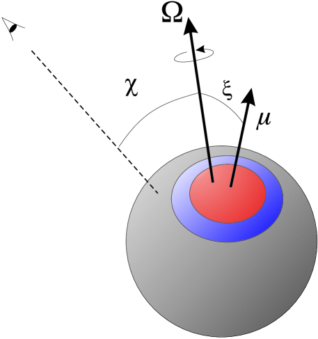
Figure 1.— A schematic view of the neutron star. ${\mathbf{\Omega}}$ and ${\mathbf{\mu}}$ are the star spin and magnetic axis, respectively. The dashed line corresponds to the line-of-sight. The two angles $\chi$ and $\xi$ are also shown. The star surface is divided into three regions: a hot polar cap (red), a warm corona (blue) and a colder zone (gray).

Monte Carlo models are computed (and stored) for the simplest geometrical case, in which the spin and the magnetic axes are aligned. As discussed in NTZ, the most general situation in which the spin and magnetic axes are at an arbitrary angle $\xi$ can be treated at the post-production level. If $\chi$ is the inclination of the line-of-sight (LOS) with respect to the star spin axis and $\alpha$ is the rotational phase angle, the co-ordinates of the points where the LOS intersects the sky can be found in terms of $\xi$, $\chi$ and $\alpha$. The pulse profile in any given energy band is then obtained by integrating over the selected range the energy-dependent counts at these positions as the star rotates (see again NTZ for details). In order to compare model lightcurves with observations, integration over energy is performed by accounting for both interstellar absorption and the detector response function. Actually, the interstellar absorption cross-section $\sigma$ and the response function $A$ depend on the photon energy at infinity $\bar{E}=E\sqrt{1-R_{S}/R_{NS}}$, where $E$ is the energy in the star frame (which is used in the Monte Carlo calculation) and $R_{S}$ is the Schwarzschild radius (we assume a Schwarzschild space-time and take $R_{NS}=10\ {\rm km}$ and $M_{NS}=1.44\ M_{\odot}$). Our model pulse profile in the $[\bar{E}_{1},\,\bar{E}_{2}]$ energy band is then proportional to

$$\int_{\bar{E}_{1}}^{\bar{E}_{2}}d\bar{E}\,\exp{[-N_{H}\sigma(\bar{E})]}A(\bar{E})N(\alpha,E)$$ (3)

where $N_{H}$ is the hydrogen column density and $N(\alpha,E)$ is the phase- and energy-dependent count rate. In the applications below we used the Morrison, & McCammon (1983) model for interstellar absorption and, since we deal with XMM-Newton observations, we adopted the EPIC-pn response function. We remark that the Monte Carlo spectral calculation is carried out assuming a flat space-time (i.e. photons propagate along straight lines), so that, apart from the gravitational redshift, no allowance is made for general-relativistic effects (see Zane, & Turolla, 2006, for a more detailed discussion). In particular, no constraints on the star mass and radius can be derived in the present case from the comparison of model and observed pulse profiles (see e.g. Leahy et al., 2008, 2009).

Finally, phase-averaged spectra are computed by summing over all phases the energy-dependent counts. Note that $0\leq\xi\leq\pi/2$, while $\chi$ is in the range $[0,\pi]$ because of the asymmetry between the north and south magnetic poles introduced by the current flow.

4. TAXP Analysis

Our first step in the study of the two TAXPs XTE J1810-197 and CXOU J164710.2-455216 was to reproduce the pulse profiles (and their time evolution) within the RCS model discussed in §3. The fit to the observed pulse profiles in different energy bands (total: $0.5\ {\rm keV}\leq E\leq 10\ {\rm keV}$, soft: $0.5\ {\rm keV}\leq E\leq 2\ {\rm keV}$, hard: $2\ {\rm keV}\leq E\leq 10\ {\rm keV}$) provides an estimate of the source parameters, including the two geometrical angles $\xi$ and $\chi$. While the twist angle, electron velocity and surface temperature may vary in the different observations (although they must be the same in the different energy bands for a given observation), the fits have to produce values of $\xi$ and $\chi$ which are at all epochs compatible with one another (to within the errors) in order to be satisfactory. We then computed the phase-averaged spectra for the two sources at the various epochs for the same sets of parameters and compared them with the observed ones. There are several reasons which led us to choose such an approach. The main one is that, as discussed in NTZ (see also Zane et al., 2009), spectral fitting alone is unable to constrain the two geometrical angles. Moreover, lightcurve fitting allows for a better control in the case in which the surface thermal map is complex and changes in time (see below).

For the present investigation, a model archive was generated beforehand. Each model was computed by evolving $N_{patch}=225,000$ photons for $N_{\Theta}\times N_{\Phi}=8\times 4=32$ surface patches ($N_{tot}=7,200,000$ photons). The parameter grids are: $0.1\leq kT\leq 0.9\ {\rm keV}$ (step $0.05\ {\rm keV}$), $0.1\leq\beta\leq 0.9$ (step $0.1$) and $0.2\,{\rm rad}\leq\Delta\phi_{N-S}\leq\,1.2\,{\rm rad}$ (step $0.1\,{\rm rad}$). Photons are collected on a $N_{\Theta_{s}}\times N_{\Phi_{s}}=10\times 10=100$ angular grid on the sky, and in $N_{E}=50$ energy bins, equally spaced in $\log E$ in the range $0.1-100\ {\rm keV}$.

The analysis proceeds as follows. We first used the principal component analysis (PCA) to explore the properties of the lightcurves as a population and to select the model within the archive that is closest to the observed one at a given epoch. This serves as the starting point for the pulse profile fitting procedure, which we performed by assuming that the whole star surface is at the same temperature. The fitting is then repeated first for the case in which the surface thermal distribution consists of a hot spot and a cooler region, and then by generating a new archive with a finer surface gridding, and applying it in the case of a surface thermal map consisting of a hot spot, a warm corona and a cooler region (see again Fig 1). Finally, the source parameters derived from the lightcurve fitting are used to confront the model and observed (phase-averaged) spectra. Phase-resolved spectral analysis, although feasible in our model and potentially important, was not attempted because the decay in flux of both sources makes the counting statistics rather poor after the first one/two observations (see Bernardini et al., 2009, for more details in the case of XTE J1810-197).

4.1. PCA

The principal component analysis is a method of multivariate statistics that allows to reduce the number of variables $X_{i}$ needed to describe a data set by introducing a new set variables, the principal components (PCs) $Z_{i}$. The PCs are linear combinations of the original variables and are such that $Z_{1}$ displays the largest variance, $Z_{2}$ the second largest, and so on. By using the PCs it is possible to describe the data set in terms of a limited number of variables, which however, carry most of the information contained in the original sample (see e.g. Zane, & Turolla, 2006, and references therein).

Synthetic lightcurves were generated for 32 phases in the range $[0,2\pi]$ and for a $9\times 9$ angular grid, $0^{\circ}\leq\xi\leq 90^{\circ}$ (step $10^{\circ}$), $0^{\circ}\leq\chi\leq 180^{\circ}$ (step $20^{\circ}$); the archive contains a total of 136323 models. Once the PCA was applied to the lightcurve set, we found that the first three PCs ($Z_{1},Z_{2},Z_{3}$) accounts for as much as $\sim 90\%$ of the sample variance. This means that the entire set is satisfactorily described in terms of just three variables instead of the original 32 (see Zane, & Turolla, 2006, for an interpretation of $Z_{1},Z_{2},Z_{3}$). A graphic representation of the lightcurves in the archive in terms of the first three PCs is shown in Fig. 2. In the same plot we also show the PC representation of the pulse profiles of XTE J1810-197 and CXOU J164710.2-455216 at the various epochs. The points corresponding to observations fall within the volume occupied by models and this guarantees that there is a combination of the parameters for which a synthetic pulse profile reproduces the data. The PC representation is also used to find the model in the archive which is closest to a given observed lightcurve, by looking for the minimum of the (squared) Euclidean distance $\sum_{i=1}^{32}(Z_{i}-Z_{i}^{obs})^{2}$ between the model and the observed pulse profile.

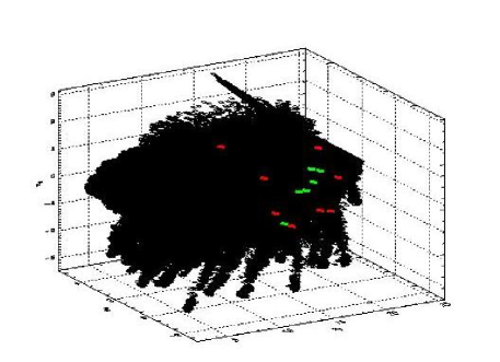
Figure 2.— Principal component representation of the simulated lightcurves in our archive (black squares) together with the observed lightcurves of XTE J1810-197 (red dots) and of CXOU J164710.2-455216 (green dots). All the pulse profiles refer to the 0.5–10 keV band.

4.2. XTE J1810-197

We considered eight XMM-Newton observations, covering the period September 2003-September 2007 for the TAXP prototype XTE J1810-197 (see Table 1 for the observation log). Only EPIC-pn data were used, and we refer to Bernardini et al. (2009), who analyzed the same observations, for all details on data extraction and reduction. All the EPIC-pn spectra were rebinned before fitting, to have at least 40 counts per bin and prevent oversampling the energy resolution by more than a factor of three.

Table 1XTE J1810-197 XMM-Newton observations

Label	OBS ID	Epoch	Exposure time (s)	total counts	background counts
Sep03	0161360301	2003-09-08	5199	60136	2903
Sep04	0164560601	2004-09-18	21306	89082	1574
Mar05	0301270501	2005-03-18	24988	54279	1760
Sep05	0301270401	2005-09-20	19787	21876	1311
Mar06	0301270301	2006-03-12	15506	12296	1197
Sep06	0406800601	2006-09-24	38505	23842	2974
Mar07	0406800701	2007-03-06	37296	21903	2215
Sep07	0504650201	2007-09-16	59014	34386	4117

4.2.1 Pulse profiles

We started our analysis by making the simplest assumption about the star surface thermal map, a uniform distribution at temperature $T$. Lightcurves were then computed in the total, soft and hard energy band for all the models in the archive. Once the model closest to each observation (and in each band) was found through the PCA, we used it as the starting point for a fit performed using an IDL script based on the minimization routine mpcurvefit.pro. Our fitting function has six free parameters, because, in addition to the twist angle, the temperature, the electron velocity, the angles $\chi$ and $\xi$, we have to include an initial phase to account for the indetermination in the position of the pulse peak. Since it is not possible to compute “on the fly” the pulse profile for a set of parameters different from those contained in the archive, lightcurves during the minimization process were obtained from those in the archive using a linear interpolation in the parameter space.

In this way we obtained a fair agreement with the observed pulse profiles ($\chi^{2}\leq 1.12$ in five out of eight observations; see Table 4), and the values of the physical parameters ($\Delta\phi_{N-S}$, $\beta$, $T$) turn out to be the same (to within the errors) for a given epoch among the different energy bands, as it needs to be. Moreover, the evolution of the twist angle and of the surface temperature follows a trend in which both quantities decrease in time as the outburst declines. This is expected if the outburst results from a sudden change in the NS magnetic structure, producing both a heating of the star surface layers and a twisting of the magnetosphere which then dies away (Thompson, Lyutikov, & Kulkarni, 2002; Beloborodov, 2009). However, the model is not acceptable since we found that the geometrical angles $\chi$ and $\xi$ change significantly from one observation to another, and even for the same observation in the different energy bands (see Fig. 3 where the parameter evolution is shown for the three energy bands). The analysis of the hard band was not carried out after September 2006, because in both the 2007 observations photons with energy $>2$ keV are only a few and, as a consequence, lightcurves are affected by large uncertainties.

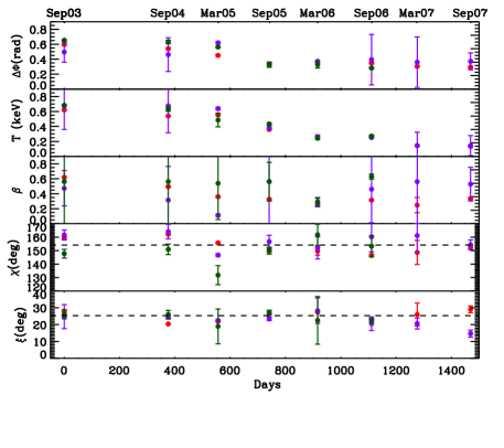
Figure 3.— Parameters evolution for XTE J1810-197, uniform surface temperature; results refer to the total (red dots), soft (blue dots) and hard (green dots) energy bands. Parameter errors are calculated by the minimization routine mpcurvefit.pro, and are at $1\sigma$. Time is computed starting from the September 2003 observation.

This shortcoming is most probably due to our oversimplifying assumption about the NS thermal map. In fact, it was shown that in the post-outburst phase the surface temperature distribution of XTE J1810-197 is complex and changes in time (Perna & Gotthelf, 2008; Bernardini et al., 2009, although a different emission model was assumed in these investigations). In order to check this, we tried different configurations, starting with a two-temperature map: a hot cap centered on one magnetic pole with the rest of the surface at a constant, cooler temperature. In this picture both temperatures as well as the emitting areas, are allowed to vary in time. While applying the one-temperature model we found that both the 2007 observations were reasonably well reproduced with a value of the (uniform) surface temperature $\sim 0.15\ {\rm keV}$, comparable to the quiescent one (see also Bernardini et al., 2009). In order to check if this fit can be further refined, we started from the September 2007 observation, freezing the colder temperature at $T_{c}=0.15\ {\rm keV}$, and letting the hot cap temperature $T_{h}$ free to vary. Since the cap area $A_{h}$ is not known a priori, nor it can be treated as a free parameter in our minimization scheme, we tried several values of $A_{h}$, corresponding to one up to eight patches of our surface grid (this means that $A_{h}$ is $n/32$ of the star surface, with $n=1,\,\ldots,\,8$). The best-estimate emitting area was then taken as the one giving the lowest reduced $\chi^{2}$ for the fit in the different trials. We verified that in all cases the same value of the cap area produces the minimum $\chi^{2}$ in all energy bands. Independent of the emitting area chosen, we always found for $T_{h}$ a value compatible with $\sim 0.15\ {\rm keV}$ for both the September and March 2007 observations.

One can then conclude that, for these two epochs, the entire star is radiating at the same temperature, or if a hot cap exists, its area is smaller than $\sim 3\,\%$ of the star surface (the size of our surface grid resolution). For these epochs we report in table 2 the values of the cold temperature obtained by using the single temperature scenario. We note that the temperature value is at the border of our grid of parameter values, so that, strictly speaking, it should be regarded as an upper limit on $T_{c}$. However, we verified that the $\chi^{2}$ steeply grows when $T_{c}$ increases above $0.15-0.16\,{\rm keV}$. Although there is no guarantee that the same is true when $T_{c}$ decreases, in the following we assume that $T_{c}\sim 0.15\,{\rm keV}$ is a satisfactory estimate for the uniform temperature at these epochs.

We then proceeded backwards in time, from September 2006 till September 2003. Again, the cooler temperature is kept fixed while several values of $A_{h}$ are tried. However, to account for the possibility that also $T_{c}$ varies, we repeated the calculation for $T_{c}=0.15,\,0.20,\,0.25,\,0.30\ {\rm keV}$, looking for the pair ($T_{c},\,A_{h}$) which gives the lowest $\chi^{2}$. Results are summarized in table 2. Although the fits improve with respect to the one-temperature model (see table 4), the two geometrical angles still change from one observation to another and also across different bands at the same epoch.

Table 2XTE J1810-197 parameters and thermal map (two-temperature model)

Epoch	$\Delta\phi_{N-S}$	$\beta$	$\xi\ (^{\circ})$	$\chi\ (^{\circ})$	$T_{h}$ (keV)	$A_{h}(\%)$	$T_{c}$ (keV)	$A_{c}(\%)$
Sep03	$0.70\pm 0.01$	$0.80\pm 0.01$	$22.7\pm 0.5$	$144.2\pm 0.6$	$0.71\pm 0.01$	$25.0\pm 3.1$	$0.30$	$75.0\pm 3.1$
Sep04	$0.67\pm 0.01$	$0.62\pm 0.02$	$20.7\pm 1.0$	$158.2\pm 0.2$	$0.55\pm 0.01$	$18.7\pm 3.1$	$0.30$	$81.3\pm 3.1$
Mar05	$0.61\pm 0.01$	$0.49\pm 0.01$	$21.6\pm 0.4$	$147.1\pm 0.6$	$0.67\pm 0.01$	$12.5\pm 3.1$	$0.25$	$87.5\pm 3.1$
Sep05	$0.47\pm 0.01$	$0.53\pm 0.05$	$23.0\pm 0.1$	$159.0\pm 1.1$	$0.42\pm 0.01$	$9.4\pm 3.1$	$0.25$	$90.6\pm 3.1$
Mar06	$0.49\pm 0.01$	$0.50\pm 0.11$	$23.5\pm 0.4$	$149.4\pm 3.5$	$0.28\pm 0.01$	$6.2\pm 3.1$	$0.15$	$93.8\pm 3.1$
Sep06	$0.43\pm 0.01$	$0.71\pm 0.16$	$21.4\pm 0.3$	$155.7\pm 1.7$	$0.28\pm 0.01$	$3.1\pm 3.1$	$0.15$	$96.9\pm 3.1$
Mar07	$0.45\pm 0.01$	$0.6\pm 0.01$	$29.8\pm 0.1$	$162.8\pm 0.1$	$-$	$-$	$0.16\pm 0.01$	$100.0$
Sep07	$0.48\pm 0.01$	$0.70\pm 0.08$	$22.4\pm 0.1$	$163.0\pm 1.7$	$-$	$-$	$0.15\pm 0.01$	$100.0$

In order to reproduce more accurately the star thermal map, we generated a new model archive, increasing the number of surface patches to $N_{\Theta}\times N_{\Phi}=50\times 4=200$. The temperature, electron velocity and twist angle are in the range $0.15\ {\rm keV}\leq T\leq 0.9\ {\rm keV}$ (step 0.15 keV), $0.1\leq\beta\leq 0.9$ (step 0.2) and $0.4\,{\rm rad}\leq\Delta\phi_{N-S}\leq 1.2\,{\rm rad}$ (step 0.2 rad), respectively. We then assumed that the star surface is divided into three zones: a hot cap at temperature $T_{h}$, a concentric warm corona at $T_{w}$ and the remaining part of the neutron star surface at a cooler temperature, $T_{c}$. Again, we began our analysis from the 2007 observations, fixing $T_{c}=0.15\ {\rm keV}$, and searching for the value of the warm temperature $T_{w}$. Every fit was repeated for twelve values of the emitting area $A_{w}=0.5\,\%,\,1\,\%,\,2\,\%,4\,\%,\,\ldots,\,20\,\%$ the total surface. We found that the reduced $\chi^{2}$ improves with the addition of a warm cap at $T_{w}\sim 0.3\ {\rm keV}$, accounting for $0.5\,\%$ of the neutron star surface (see table 3). We stress that this value is below the resolution of our previous grid, so the two results are consistent with each other.

We then considered the two 2006 observations; in the two-temperature model based on the previous archive, these were reasonably reproduced with $T_{c}=0.15\ {\rm keV}$ and $T_{h}\sim 0.3\ {\rm keV}$ (note that $T_{h}$ for the two-temperature model corresponds to $T_{w}$ in the present case). For these two observations we repeated the fit, fixing $T_{c}$ at $0.15\ {\rm keV}$ while leaving $T_{w}$ free to vary. The size of the emitting area was estimated by following the same procedure discussed above. We found an almost constant value, $T_{w}\sim 0.3\ {\rm keV}$, between March 2006 and September 2007, while the emitting area decreases in time. Also, we found no need for a further component at $T_{h}$ at these epochs. On the other hand, results for the two-temperature case (see table 2) show the presence of a component with temperature higher than $0.3\ {\rm keV}$, in the period between September 2003 and September 2005 (while the cooler one varies between $0.25$ and $0.30\ {\rm keV}$). It is tempting to associate this to a transient hot cap that appears only in the first period after the outburst, superimposed to the other, longer-lived emitting zones.

To test this possibility, we re-fitted the first four observations by fixing the coldest temperature at $T_{c}=0.15\ {\rm keV}$, the warmer one at $T_{w}=0.3\ {\rm keV}$, and leaving only the hotter temperature free to vary. For each observation the pulse profile fits were computed for every combination of $A_{h}$ and $A_{w}$ chosen among the twelve values in the range $0.5\,\%$– $20\,\%$ introduced before, and looking for the minimum of the reduced $\chi^{2}$. Results of the lightcurve fitting at different epochs are listed in table 3 and shown in Fig. 4, while the reduced $\chi^{2}$ for the three thermal distributions is reported in table 4.

Table 3XTE J1810-197 parameters and thermal map (three-temperature model)

Epoch	$\Delta\phi_{N-S}$	$\beta$	$\xi\ (^{\circ})$	$\chi\ (^{\circ})$	$T_{h}$ (keV)	$T_{w}$ (keV)	$T_{c}$ (keV)	$A_{h}(\%)$	$A_{w}(\%)$
Sep 03	$0.80^{+0.05}_{-0.11}$	$0.70^{+0.08}_{-0.06}$	$27.8^{+4.6}_{-3.1}$	$145.3^{+4.7}_{-2.5}$	$0.62^{+0.14}_{-0.14}$	$0.30$	$0.15$	$8.\pm 0.5$	$16.\pm 0.5$
Sep 04	$0.79^{+0.07}_{-0.08}$	$0.78^{+0.09}_{-0.23}$	$16.2^{+4.2}_{-5.9}$	$140.8^{+5.8}_{-2.6}$	$0.49^{+0.03}_{-0.22}$	$0.30$	$0.15$	$6.\pm 0.5$	$14.\pm 0.5$
Mar 05	$0.62^{+0.03}_{-0.03}$	$0.51^{+0.07}_{-0.09}$	$22.2^{+5.4}_{-13.1}$	$146.9^{+7.9}_{-1.8}$	$0.49^{+0.01}_{-0.04}$	$0.30$	$0.15$	$4.\pm 0.5$	$14.\pm 0.5$
Sep 05	$0.53^{+0.10}_{-0.09}$	$0.50^{+0.11}_{-0.19}$	$21.4^{+10.3}_{-20.0}$	$154.4^{+13.9}_{-9.5}$	$0.52^{-}_{-}$	$0.30$	$0.15$	$2.\pm 0.5$	$10.\pm 0.5$
Mar 06	$0.46^{+0.08}_{-0.04}$	$0.73^{+0.20}_{0.20}$	$18.5^{18.0}_{-17.2}$	$143.0^{+7.9}_{-7.5}$	-	$0.29^{+0.17}_{-0.03}$	$0.15$	-	$6.\pm 0.5$
Sep 06	$0.54^{+0.04}_{-0.03}$	$0.42^{+0.13}_{-0.12}$	$22.4^{+12.3}_{-20.0}$	$150.2^{+14.3}_{-9.5}$	-	$0.30^{-}_{-}$	$0.15$	-	$2.\pm 0.5$
Mar 07	$0.49^{+0.20}_{-0.05}$	$0.43^{+0.13}_{-0.12}$	$30.0^{+12.3}_{-20.0}$	$153.9^{+19.6}_{-16.0}$	-	$0.29^{-}_{-}$	$0.15$	-	$0.5\pm 0.5$
Sep 07	$0.47^{+0.07}_{-0.04}$	$0.50^{+0.09}_{-0.15}$	$22.7^{+16.4}_{-20.0}$	$145.8^{+16.4}_{-9.5}$	-	$0.31^{-}_{-}$	$0.15$	-	$0.5\pm 0.5$

Table 4Reduced $\chi^{2}$ for XTE J1810-197

Epoch	$\chi^{2}_{red}$	$\chi^{2}_{red}$	$\chi^{2}_{red}$	$\chi^{2}_{red}$	$T$
	(1T)	(2T)	(3T)	(XSPEC)	(keV)
Sep 03	1.72	1.58	0.12	1.22	-
Sep 04	0.66	0.42	0.36	1.93	-
Mar 05	1.02	0.98	0.79	1.50	-
Sep 05	1.06	0.40	0.39	1.52	$0.53_{-0.06}^{+0.07}$
Mar 06	2.94	1.70	1.25	1.34	-
Sep 06	0.94	0.38	0.35	1.36	$0.31_{-0.01}^{+0.03}$
Mar 07	2.88	2.88	2.37	1.08	$0.29_{-0.02}^{+0.04}$
Sep 07	1.12	1.12	0.96	1.29	$0.31_{-0.01}^{+0.01}$

A worry may arise whether the best-fitting values obtained from the minimization routine correspond indeed to absolute minima of the reduced $\chi^{2}$. In order to check this, and visually inspect the shape of the $\chi^{2}$ curve close to the solution, we computed and plotted the reduced $\chi^{2}$ leaving, in turn, only one parameter free and freezing the remaining five at their best-fit values. This also allowed us to obtain a more reliable estimate of the parameter errors which were computed by looking, as usual, for the parameter change which corresponds to a $1\sigma$ confidence level (and reported in table 3).

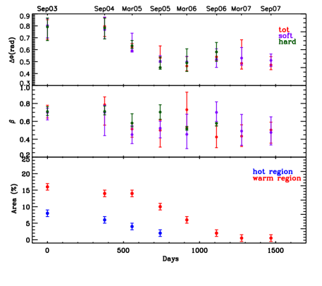
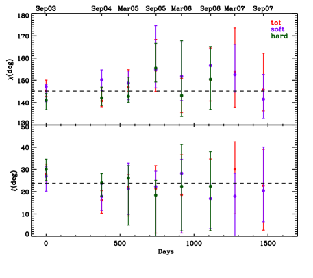
Figure 4.— Parameters evolution for XTE J1810-197, three temperature model. Left (from top to bottom): twist angle ($\Delta\phi$), bulk velocity ($\beta$) and area of the different emitting regions. Right: the two geometrical angles, $\chi$ and $\xi$. Details as in fig. 3.

We found that all values obtained with the mpcurvefit.pro routine indeed correspond to minima of the reduced $\chi^{2}$ curve, with the exception of the temperature(s), for which there are observations (or energy bands) with very flat $\chi^{2}$ curves (see Fig. 5). In particular, for the September 2005 observation the curve obtained varying $T_{h}$ is flat in all the three energy bands. Also the curves relative to $T_{w}$ for the September 2006, March 2007 and September 2007 observations have the same problem. This can be understood by noting that in all these observations the size of the hot/warm region accounts for only $<2\,\%$ of the total neutron star surface: temperature changes in such a small emitting area can hardly influence the fit. In addition, for the March 2005 and March 2006 observations the reduced $\chi^{2}$ curve relative to one of the temperatures is flat, but this occurs only for one of the three energy bands. The first case concerns the hot temperature and the soft band, the second the warm temperature and the hard band. As we discussed above, when the hot (warm) area shrinks it affects little the pulse profile; this shows up first in the energy band in which its emission contributes less, i.e. the soft (hard) band.

Figure 5.— Two examples of the different behavior of the reduced $\chi^{2}$ for the warm temperature. The top curve refers to the March 2006 observation (soft band) and exhibits a well-defined minimum. The bottom curve (September 2006 observation, total band) is so flat to make it impossible to gauge the best-fitting value and its errors.

Given these findings, we concluded that lightcurve analysis by itself is unable to yield an unique temperature value for the September 2005, the September 2006, and both the 2007 observations. On the other hand, spectral analysis is more sensitive to temperature variations, so that it is possible to infer a temperature value also in these cases. As it will be discussed in the next section, by combining the two techniques we can remove most of the uncertainties and validate the three temperature model presented so far (see sec. 4.2.2 for details).

There are several physical implications than can be drawn from our model. The TAXP is seen at an angle $\chi=148^{\circ+7}_{-9}$ with respect to the spin axis. The misalignment between the spin axis and the magnetic axis is $\xi=23^{\circ+15}_{-11}$. These values of the two angles, and the corresponding errors, are calculated from the weighted average in the three energy bands. To get a quantitative confirmation that $\chi$ and $\xi$ do not change in time, we fitted a constant through the values of each angle as derived from the lightcurves fitting at the different epochs and found that the null hypothesis probability is $<1\,\%$. We note that, formally, the misalignment between the spin and the magnetic axis is compatible with being zero at the $3\sigma$ level. Low values of $\xi$ produce, however, models with pulsed fractions quite smaller than the observed ones and, despite $\xi\sim 0$ might be still statistically acceptable, we regard this possibility as unlikely because the amplitude is the main feature which characterizes the pulse, as the PCA shows (see §4.1, the first principal component, $Z_{1}$, is, in fact, directly related to the amplitude).

It emerges a scenario in which, before the outburst, the NS surface radiates uniformly at a temperature $T_{c}\sim 0.15\ {\rm keV}$. Soon after the burst the thermal map of XTE J1810-197 substantially changes. The region around the magnetic north pole is heated, reaches a temperature of $\sim 0.7\ {\rm keV}$ and covers an area $\sim 8\%$ of the total star surface. This hot spot is surrounded by a warmer corona at $\sim 0.3$ keV, that covers a further $\sim 16\%$ of the surface. During the subsequent evolution, the hot cap decreases in size and temperature until the March 2006 observation, when it becomes too small and cold to be distinguished from the surrounding warm corona. The warm region remains almost constant until September 2005, then decreases in size, and becomes a cap in March 2006, following the hot spot disappearance. In September 2007 (our last observation for XTE J1810-197) the warm cap is still visible, even if its area is down to only $\sim 0.5\%$ of the total. The twist angle is highest at the beginning of the outburst (September 2003) and then steadily decreases until it reaches a more or less constant value around September 2005. The electron velocity does not show large variations in time and stays about constant at $\beta\sim 0.5$.

Synthetic and observed lightcurves (in the total band) are shown in Fig 6, together with the fit residuals. We note that the residuals exhibit a well-defined, oscillatory pattern at all epochs. In our scenario, this can be possibly associated to a more complicated thermal map, of which our 3T model is a first-order approximation (e.g. non-circular shape of the hotter regions, off-centering of the hot and warm areas). However, as discussed in some more detail in § 5, no further refinement of the surface thermal map will be attempted here. Since XTE J1810-197 pulse profiles are fairly sinusoidal, we can compute the pulsed fraction and its evolution in time at different energies. The comparison of model results with data is shown in Fig. 7.

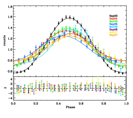
Figure 6.— Synthetic (3T model) and observed pulse profiles for XTE J1810-197 in the total energy band. Solid lines represent the best-fitting model, dots the observed lightcurves. Initial phases are arbitrary. The lower panel shows the residuals.

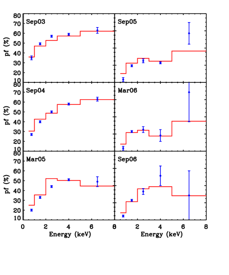
Figure 7.— The variation of XTE J1810-197 pulsed fraction with energy at different epochs. The red line refers to the model, blue dots to observations (errors are at $1\sigma$).

4.2.2 Spectra

In order to verify if the thermal map inferred from the pulse profile fits is reasonable, and in order to remove the uncertainties in the value of the temperature at certain epochs (see § 4.2.1), we examined the source spectra. The goal is to check if the parameters derived from our lightcurve analysis (twist angle, bulk velocity, size and temperature of the three emitting areas, and the angles $\chi$, $\xi$) can also reproduce the spectral evolution of XTE J1810-197 during the outburst decay. To this end, we used the ntzang model that was implemented in XSPEC by Nobili, Turolla, & Zane (2008, the model is not currently available in the public library, but it can be obtained from the authors upon request). The ntzang XSPEC model has the same free parameters as those used in our fits of the pulse profiles. In addition it contains the normalization and the column density. We caveat that, since this XSPEC model was created by assuming that the entire star surface emits at uniform temperature, strictly speaking is not directly suited to the present case. As an approximation, we fitted the spectra by adding together three (absorbed) ntzang models, each associated to one of the three thermal components, at temperatures $T_{h}$, $T_{w}$ and $T_{c}$, respectively. At each epoch the fit was performed by freezing $\Delta\phi_{N-S}$, $\beta$, $T$, $\chi$ and $\xi$ at the values derived from the fit of the lightcurve in the total energy band (see §4.2.1), while the three model normalizations (which are related to the emitting areas) were left free to vary. We also required that the column density, $N_{H}$, is the same for all the three spectral components and for all epochs. Since for the September 2005, the September 2006 and both the 2007 observations the lightcurve analysis did not return an unique value for the hotter temperature, we also left this parameter free to vary in these four observations. In all these cases, we found that the fit converges to a value of the temperature close to the best-fitting value obtained from the lightcurve analysis (see table 4). Moreover, the reduced $\chi^{2}$ significantly worsens by varying the temperature, meaning that the spectra are much more sensitive to the presence of these components. Results are shown in Fig. 8, while the reduced $\chi^{2}$ for the fits at the various epochs are reported in Tab. 4. The value of the column density is found to be $N_{H}=(7.73\pm 0.50)\times 10^{21}\ {\rm cm^{-2}}$, compatible at the $1.5\sigma$ level with the one obtained by Bernardini et al. (2009) with the 3 BB model, $N_{H}=(6.3\pm 0.5)\times 10^{21}\ {\rm cm^{-2}}$. We remark that, in assessing the goodness of the fits, only the normalizations of the three components (plus $N_{H}$) are free to vary; all the other model parameters are frozen at the best values obtained from the pulse profile analysis. Under these conditions, we regard the agreement of our model with observed spectra as quite satisfactory. We note that the presence of systematic residuals at high energies (above 7–8 keV) may be hinted in the fits of the three earlier observations (see Fig. 8). As discussed by Bernardini et al. (2009) they may be related to a harder spectral component which is however only marginally significant ($3.2\sigma$ confidence level) and quite unconstrained. Given that the high-energy residuals are comparable to (or smaller than) those of the 3 BB model used by Bernardini et al. (2009), we conclude that a hard tail is not significant also in our modelling and we did not attempt to include it in our fits.

We checked how the reduced $\chi^{2}$ for the spectral fit changes when the (frozen) parameters are varied within $\sim 2\sigma$ from their best-fit value (as from the pulse fitting). This has been done changing one parameter at a time. We found that indeed the $\chi^{2}$ increases quite smoothly in response to the change of each parameter, with the exception of $\chi$ and $\xi$. This is not surprising, since we knew already that the spectrum is not much sensitive to the geometry. We also tried a fit leaving all the parameters free, apart from the two geometrical angles which were held fixed at their best-fit values. The fit returns parameter values which are the same, within the errors, as those derived from the pulse fitting and comparable values of the reduced $\chi^{2}$, implying that the solution we presented is indeed a global $\chi^{2}$ minimum. The same procedure and the same conclusions hold also in the case of CXOU 164710.2-455216 (see § 4.3.2).

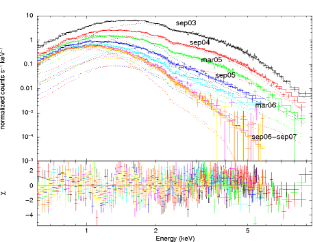
Figure 8.— Spectral evolution in the eight XMM-Newton observations of XTE J1810-197. Solid lines represent the model, while dotted lines refer to the single ntzang components (see text for details). Residuals are shown in the lower panel.

4.3. CXOU J164710.2-455216

Having verified that our model can provide a reasonable interpretation for the post-outburst timing and spectral evolution of TAXP prototype XTE J1810-197, we applied it to CXOU J164710.2-455216, the other transient AXP for which a large enough number of XMM-Newton observations covering the outburst decay are available (see table 5 for details). During September 2006 the pn and MOS cameras were set in full window imaging mode with a thick filter (time resolution = $73.3\times 10^{-3}$ s and 2.6 s for the pn and MOS, respectively), while all other observations were in a large and small window imaging mode with a medium filter (time resolution = $4.76\times 10^{-2}$ s and 0.3 s for the pn and MOS, respectively). To extract more than 90% of the source counts, we accumulated a one-dimensional image and fitted the 1D photon distribution with a Gaussian. Then, we extracted the source photons from a circular region of radius 40″(smaller than the canonical 55″, corresponding to 90% of the source photons, in order to minimize the contamination from nearby sources in the Westerlund 1 cluster) centered at the Gaussian centroid. The background for the spectral analysis was obtained (within the same pn CCD where the source lies and a different CCD for the MOS) from an annular region (inner and outer radii of 45″and 65″, respectively) centered at the best source position. In the timing analysis, the background was estimated from a circular region of the same size as that of the source. EPIC-pn spectra were processed as in the case of XTE J1810-197 (see §4.2).

Table 5CXOU J164710.2-455216 XMM-Newton observations

Label	OBS ID	Epoch	Exposure time (s)	total counts	background counts
Sep 06	0311792001	2006-09-22	26780	56934	1709
Feb 07	0410580601	2007-02-17	14740	18734	1264
Aug 07	0505290201	2007-08-19	16020	11710	2384
Feb 08	0505290301	2008-02-15	9080	4618	1131
Aug 08	0555350101	2008-08-20	26360	7357	1689
Aug 09	0604380101	2009-08-24	33030	4974	1959

4.3.1 Pulse profiles

The analysis of the pulse profiles of CXOU J164710.2-455216 follows closely that presented in §4.2.1. In particular, we first tried a single temperature and then a two-temperature model, encountering the same problems we found for XTE J1810-197. Finally, we applied a three-zone thermal map and this provided reasonable fits for the lightcurves, and the angles $\chi$ and $\xi$ were not found to vary in the same observation for the different energy bands and for different epochs. We did not attempt to fit the pulse profiles in the hard band after the February 2007 observation because of the very few counts at energies $>2$ keV. As for XTE J1810-197 we started the analysis from the last observation (August 2009) assuming a thermal map comprising a hot cap centered on the magnetic pole at temperature $T_{h}$, a concentric warm corona at $T_{w}$ and the rest of the neutron star at the colder temperature $T_{c}$. Every fit was repeated for ten values of the hot cap area $A_{h}=0.5\,\%,\,1\,\%,\,2\,\%,4\,\%,\,\ldots,\,16\,\%$ (of the total surface) and for 20 values of the warm corona area $A_{w}=0.5\,\%,\,1\,\%,\,2\,\%,4\,\%,\,\ldots,\,30\,\%$. Moreover, lightcurves fits were iterated for two values of the cold temperature $T_{c}=0.15,0.30$ keV and also for two values of the warm temperature $T_{w}=0.30,0.45$ keV. The hotter temperature was left free to vary. We found that in the last two observations, independent of the hot cap size, $T_{h}$ is always $\sim 0.45$ keV, nearly indistinguishable from the temperature of the warm corona obtained from the fit. We concluded that, at least for our present surface grid resolution, in the last two observations there are only two thermal components that contribute to the emission, the cold and warm ones, and repeated the fit leaving $T_{w}$ free to vary. Results are reported in table 6 and plotted in Fig. 9, while a comparison of the reduced $\chi^{2}$ for the three thermal distributions is given in table 7. Errors listed in the tables have the same meaning as in the case of XTE J1810-197. Again, when the spot at $T_{h}$ becomes very small its temperature can not be determined unambiguously.

Table 6CXOU J164710.2-455216 parameters and thermal map (three-temperature model)

Epoch	$\Delta\phi_{N-S}$	$\beta$	$\xi\ (^{\circ})$	$\chi\ (^{\circ})$	$T_{h}$ (keV)	$T_{w}$ (keV)	$T_{c}$ (keV)	$A_{h}(\%)$	$A_{w}(\%)$
Sep 06	$1.12^{+0.08}_{-0.14}$	$0.18^{+0.03}_{-0.03}$	$83.5^{+1.0}_{-1.4}$	$20.8^{+0.1}_{-0.5}$	$0.70^{+0.20}_{-0.11}$	$0.45$	$0.15$	$8.\pm 0.5$	$22.\pm 0.5$
Feb 07	$1.07^{+0.05}_{-0.10}$	$0.19^{+0.02}_{-0.03}$	$80.0^{+2.7}_{-2.1}$	$23.2^{+1.7}_{-1.7}$	$0.64^{+0.16}_{-0.06}$	$0.45$	$0.15$	$6.\pm 0.5$	$24.\pm 0.5$
Aug 07	$1.00^{+0.18}_{-0.06}$	$0.15^{+0.02}_{-0.05}$	$82.1^{+1.1}_{-1.1}$	$19.2^{+2.7}_{-1.3}$	$0.63^{+0.18}_{-0.10}$	$0.45$	$0.15$	$4.\pm 0.5$	$26.\pm 0.5$
Feb 08	$0.77^{+0.21}_{-0.12}$	$0.20^{+0.05}_{-0.09}$	$85.7^{+2.7}_{-4.1}$	$20.4^{+7.2}_{-0.7}$	$0.62^{-}_{-}$	$0.45$	$0.15$	$2.\pm 0.5$	$28.\pm 0.5$
Aug 08	$0.65^{+0.12}_{-0.07}$	$0.70^{+0.05}_{-0.05}$	$80.1^{+2.7}_{-9.7}$	$28.4^{+4.9}_{-7.3}$	-	$0.49^{+0.02}_{-0.05}$	$0.15$	-	$30.\pm 0.5$
Aug 09	$0.55^{+0.11}_{-0.10}$	$0.79^{+0.06}_{-0.06}$	$87.0^{+9.7}_{-10.9}$	$25.5^{+4.9}_{-10.}$	-	$0.46^{+0.05}_{-0.05}$	$0.15$	-	$30.\pm 0.5$

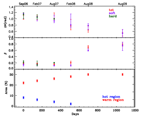
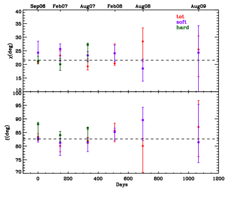
Figure 9.— Same as in Fig. 4 for the TAXP CXOU J164710.2-455216; here time is computed starting from the September 2006 observation.

According to our model, CXOU J164710.2-4552116 is viewed at an angle $\chi=23^{\circ+4}_{-3}$ with respect to its spin axis. The spin and the magnetic axes are almost orthogonal, $\xi=84^{\circ+5}_{-3}$. This is a quite peculiar condition, and it seems to be the only one capable of explaining the characteristic three-peaked shape of the observed lightcurves within the present model. As for XTE J1810-197 values and errors for both angles are calculated as the weighted average of parameters in the three energy bands. Also in this case the probability that $\chi$ and $\xi$ are not constant in time is $<1\%$.

Soon after the burst the thermal map of CXOU J164710.2-455216 consists of three regions at different temperatures. The hottest region, around the north magnetic pole, has a temperature $T_{h}\sim 0.7\ {\rm keV}$, and its area is $\sim 8\%$ of the total. This hot spot decreases in temperature and size as time elapses, until February 2008. In August 2008 the hot cap becomes so small in size and its temperature so close to that of the warm corona, that it is impossible to distinguish between the two regions. The warm corona has a temperature of $\sim 0.45\ {\rm keV}$, which remains about constant during the three years of observations. In this case the corona area slightly increases with time, starting from $\sim 20\%$ and reaching $\sim 30\%$ of the NS surface. The third region has a lower temperature $T_{c}\sim 0.15\ {\rm keV}$ and its area remains constant at $\sim 70\%$ of the total. The twist angle is $\sim 1.12$ rad soon after the burst, and it decreases with time. There are hints that its decay is slower until August 2007, then proceeds faster. The electron velocity is about the same at all epoch ($\beta\sim 0.2$), apart from the last two observations in which it strongly increases. This variation may be related to the change in the pulse shape (from three-peaked to single-peaked) and also to the increase of the pulsed fraction.

A comparison between the observed and model pulse profiles is shown in Fig. 10. Because of the inherent complexity and drastic time evolution of CXOU J164710.2-455216 lightcurves, the agreement is not as good as for XTE J1810-197. The fact that lightcurve fits return $\chi^{2}$ values not much higher than those of XTE J1810-197 (compare Tab. 4 and 7) reflects the larger uncertainties in the phase-binned source counts. We also note that the errors on the geometrical angles for CXOU J164710.2-455216 are smaller than those derived for XTE J1810-197, despite the worst agreement (see Tab. 3 and 6). This is most probably due to the different shapes of the pulses in the two sources. Because of the very peculiar lightcurve of CXOU J164710.2-455216, which can be reproduced by our model only invoking a nearly orthogonal rotator, even small depatures of $\xi$ and $\chi$ from their best-fit values results in a rapid growth of the $\chi^{2}$. This does not occur for the rather sinusoidal pulse of XTE J1810-197 since the model can produce lightcurves of more or less the right shape in a wider range of angles.

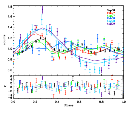
Figure 10.— Same as in Fig. 6 for CXOU J164710.2-455216; computed pulse profiles refer to the 3T model and initial phases are arbitrary.

Besides being of limited use because of the complex shape of the pulse, the pulsed fraction analysis was hindered by the lower count rate, especially at low energies and was not pursued further for this source. As in XTE J1810-197, we checked that the values obtained from the minimization routine indeed correspond to minima of the reduced $\chi^{2}$s. Again we froze five of the six parameters to the value obtained with the mpcurvefit.pro minimization routine, and calculated the reduced $\chi^{2}$ around its minimum by varying the free parameter. The procedure was repeated for all parameters and all observations in the three energy bands. Again, for all parameters but the temperature, results obtained with the mpcurvefit.pro routine indeed correspond to the minima of the reduced $\chi^{2}$ curve. There is one observation for which the $\chi^{2}$ curve relative to the hot temperature is very flat for all the energy bands. This is the August 2008 observation, for which the size of the emitting area accounts for just $2\%$ of the total neutron star surface. As in XTE J1810-197, we conclude that the fit is not very sensitive to the temperature variation for very small emitting areas. On the other hand, like in the previous case, it was possible to infer a value for the August 2008 hot temperature using the spectral analysis (see sect. 4.3.2).

Table 7Reduced $\chi^{2}$ for CXOU J164710.2-455216

Epoch	$\chi^{2}_{red}$	$\chi^{2}_{red}$	$\chi^{2}_{red}$	$\chi^{2}_{red}$	$T$
	(1T)	(2T)	(3T)	(XSPEC)	(keV)
Sep 06	1.05	0.86	0.31	1.24	-
Feb 07	1.32	0.76	0.65	0.83	-
Aug 07	0.97	0.91	0.44	1.01	-
Feb 08	1.45	1.12	0.63	1.08	$0.62^{+0.06}_{-0.09}$
Aug 08	1.45	1.23	0.79	1.23	-
Aug 09	2.03	1.97	1.52	1.36	-

4.3.2 Spectra

The spectral analysis for CXOU J164710.2-455216 was carried out using the same approach discussed in §4.2.2. We fitted three ntzang components, each representative of an emitting region at different temperature, and froze all parameters apart from the three normalizations and $N_{H}$ (which were forced to be the same for all the components and for all epochs). Moreover, since the lightcurve analysis the February 2008 observation failed to provide an unambiguous value for the hot temperature, also this parameter was left free to vary. Results are shown in Fig. 11. Given the approach we used for the fit, the agreement is quite satisfactory (reduced $\chi^{2}$ are listed if Tab. 7). Systematic residuals at low (1–2 keV) energies are however present, especially in the September 2006, August 2007 and August 2008 observations. $N_{H}$ is found to be $(2.14\pm 0.015)\times 10^{22}\ {\rm cm^{-2}}$, somewhat higher than that derived by Naik et al. (2008), $N_{H}=(1.73\pm 0.03)\times 10^{22}\ {\rm cm^{-2}}$.

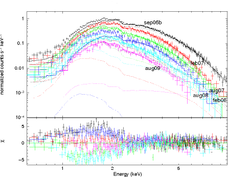
Figure 11.— Same as in Fig. 8 for the six XMM-Newton observations of CXOU J164710.2-455216.

5. Discussion

The simultaneous study of the timing and spectral characteristics of the transient AXPs XTE J1810-197 and CXOU J164710.2-455216 presented in this paper shows that the post-burst evolution of two sources share a number of similar properties. In particular, the long-term variability of the pulse profiles and spectra appears to be (semi)quantitatively consistent with a scenario in which the star surface thermal distribution and magnetospheric properties progressively change in time. Our results were derived within the twisted magnetosphere model for magnetars and support a picture in which the twist affects only a small bundle of closed field lines around one of the magnetic poles. As discussed by Beloborodov (2009), if the twist is initially confined along the magnetic axis, the returning currents hit a limited portion of the star surface (typically a polar cap), which becomes hotter. In this scenario the post-outburst evolution is related to the twist decay, during which the bundle shrinks, and the heated region decreases both in size and temperature. We found evidence for a cooling/shrinking of the heated polar cap in both sources, together with a decrease of the twist angle. It should be noted that our magnetospheric model assumes a global twist, since no spectral calculations are currently available for a localized twist.

Within this common framework, there are nonetheless differences between the two TAXPs. For XTE J1810-197 we found that the star thermal map comprises three regions: a hot cap, a surrounding warm corona, and the rest of the surface at a colder temperature. The hot cap decreases in size and temperature until it becomes indistinguishable from the corona around March 2006. Also the warm corona shrinks, although its temperature stays about constant at $\sim 0.3\ {\rm keV}$. It becomes a cap in March 2006 and it is still visible in our last observation (September 2007) although its size is down to $0.5\%$ of the entire surface. The rest of the surface remains at a temperature comparable to the quiescent one (as measured by ROSAT) during the entire evolution, indicating that the outburst likely involved only a fraction of the star surface. Bernardini et al. (2009) obtained similar results using a 3BB model, although they did not attempt to locate the different emitting regions on the star surface nor to fit the pulse profiles. In their (purely spectral) analysis the hot region is visible slightly longer (until March 2006); the reason for the difference with respect to our results being most probably the resolution of our surface grid. Moreover, in our case the hot temperature decrease is more pronounced. The twist angle decreases from $\sim 0.8$ rad to $\sim 0.5$ rad during the first two years, and then it remains roughly constant.

Much as in the case of XTE J1810-197, the thermal map of CXOU J164710.2-455216 is well reproduced by three different regions. However, while the evolution of the hot cap is similar, i.e. it decreases in size and temperature until it disappears in the August 2008 observation, the behavior of the warm corona is different. Now the warm temperature remains constant at $\sim 0.45\ {\rm keV}$ and the area increases. Actually, the area of the “hot+warm” region is constant and covers about $\sim 30\%$ of the surface, while the remaining $\sim 70\%$ is at a constant cooler temperature, $\sim 0.15\ {\rm keV}$. This is suggestive of a picture in which the ”quiescent” state of the source is characterized by a two-temperature map, with a warm polar region superposed to the cooler surface. The outburst might have heated a portion of the warm cap, producing the hot zone which then cooled off. It is intriguing to notice that the disappearance of the hot spot occurs at the same time (August 2008) at which the pulse profile dramatically changed, switching from a three-peaked to a single-peaked pattern. A quasi-sinusoidal shape of the lightcurve was observed when the source was in quiescence Israel et al. (2007). However, at that time the pulsed fraction was nearly 100% above 4 keV, likely indicating the presence of a small hot spot which is periodically occulted as the star rotates. This is in agreement with our finding that this TAXP is a nearly orthogonal rotator. Whether CXOU J164710.2-455216 is presently approaching quiescence is unclear. If this is the case, its quiescent state is different from that observed in 2005 and also from that of XTE J1810-197.

It is worth stressing that our claim that the temperature does not change spatially in each of the regions should not be taken literally. The assumption that the surface can be divided in three (or two) thermal regions was mainly introduced to simplify the calculations while catching the essential features of the model. A smooth temperature variation within a zone is likely to be present. However, it is difficult to reconcile the observed pulsed fraction of XTE J1810-197 in the September 2006 observation ($\gtrsim 10\%$, see Fig. 7) even accounting for the temperature gradient induced by the large-scale dipolar field. This may be an indication that, as our analysis shows, there is a residual twist even in the quiescent state.

In this respect we note that our spectral calculation is based on a rather fine subdivision of the star surface ($50\times 4$ patches in the final version of the archive), so we could have produced pulse profiles for arbitrary complicated thermal maps. The motivation of our choice of the thermal distribution (a hot polar cap and a warm a corona superimposed to the colder surface) is threefold: i) a model based on two thermal components, originating from a hot cap and a warm corona, was successfully applied to XTE J1810-197 by Perna & Gotthelf (2008); ii) inclusion of a third, colder component in the spectrum of the same source was shown to be statistically significant by Bernardini et al. (2009); and iii) it is consistent with theoretical predictions for a twisted magnetosphere in an AXP (Beloborodov, 2009, see above). In addition, this is the simplest map for which we were able to obtain constant values, to within the errors, for the two geometrical angles $\chi$ and $\xi$ during the entire period covered by the observations.

In their analysis of XTE J1810-197, Perna & Gotthelf (2008) assumed that the X-rays come from two concentric regions with varying temperatures and areas, each emitting a blackbody spectrum; the rest of the surface was taken to be at zero temperature. They derived the angles $\chi$ and $\xi$, and, although their solution is not unique, they claim that the pair $\chi\sim 53^{\circ}$, $\xi\sim 23^{\circ}$ is favored. While this value of $\xi$ coincides with our estimate, the two values of the inclination of the line-of-sight are in substantial disagreement. Also the emitting areas of the hot/warm region and their temperatures turn out to be different in the two cases. Their estimate of the hot temperature is always higher than ours and the size of the warm corona is not monotonically decreasing. We remark that quantitative differences are to be expected given the different assumed spectral models (blackbody vs. RCS); moreover because Perna & Gotthelf (2008) did not include a colder region.

Finally, we caveat that our analysis relies on a number of simplifying assumptions. We already mentioned that the synthetic spectra we used were obtained with the Monte Carlo code by Nobili, Turolla, & Zane (2008), which was designed to solve radiation transport in a globally twisted magnetosphere. Even though we took thermal photons to originate mostly in a limited polar region, this does not self-consistently describe resonant up-scattering in a magnetosphere where only a limited bundle of field lines is actually twisted, as is probably the case in AXPs Beloborodov (2009). Moreover, as we discussed in §4.2.2, the ntzang XSPEC model is available only in tabular form and it was created assuming emission at constant temperature from the entire star surface. As such, it is not suited to be applied directly to the present case. As a compromise, we decided to fit the spectra by adding together two/three (absorbed) ntzang components, each associated to one of the emitting regions, at temperatures $T_{h}$, $T_{w}$ and $T_{c}$, respectively. While this procedure works (and is routinely employed) in the case of blackbody spectra, it is expected to be only approximately correct when different ntzang components are added together. The reason is that the effects of resonant scattering on thermal photons depends on the location of the primary emission, since the magnetospheric electron density is not isotropic. As a consequence, assuming thermal emission from a cap of limited size or from the entire star, even if the two are taken at the same temperature, will give rise to different spectra. We checked this approximation for all the spectra we analyzed, finding that the maximum relative error is $\sim 0.6$, while the energy-averaged error is always between 0.2 and 0.4 both for XTE J1810-197 and CXOU J164710.2-455216. An example is shown in Fig 12. Although we are aware that this is not optimal, it provides a reasonable way to describe radiation coming from a magnetar with non-uniform thermal emission within the context of our model.

Figure 12.— Comparison between the spectrum obtained adding three single ntzang model (red) and the spectrum of a neutron star with a thermal map consisting of three regions at different temperatures (black). The two spectra are relative to the September 2004 observation of XTE J1810-197.

6. Conclusions

The monitoring of the two TAXPs XTE J1810-197 and CXOU J164710.2-455216, carried out with XMM-Newton in recent years, gave us the possibility to test the twisted magnetosphere model and understand how the physical parameters in the two sources change during the post-outburst evolution. We summarize our main findings below, remarking again that they were obtained under a number of assumptions (e.g. globally twisted field, three temperature thermal map).

• Soon after the outburst onset the surface thermal distribution in XTE J1810-197 and CXOU J164710.2-455216 is well described by three components: a hot cap, a surrounding warm corona while the rest of the neutron star surface is at a lower temperature.

• The analysis of the pulse profile evolution for XTE J1810-197 revealed that both the hot cap and the warm corona decrease in size so that in the last observation (September 2007) virtually all the neutron star surface emits at a temperature compatible with the quiescent one.

• The same analysis for CXOU J164710.2-455216 showed that the hot cap decreases in temperature and size, while the warm corona remains constant in temperature while it increases in size. In the last two observations we examined (August 2008 and August 2009) the source thermal map comprises a hot cap covering $\sim 30\%$ of the neutron star surface, while the remaining surface is cooler. There are hints that this could be the quiescent state of the TAXP.

• For both sources the twist angle is highest at the outburst onset and then monotonically decreases in time until it reaches a nearly constant, non-zero value.

• The same model configuration which best-fits the observed pulse profiles (thermal map, twist angle, electron bulk velocity, and geometrical angles) provides a reasonable description of XMM-Newton spectra in the 0.1–10 keV band for both sources.

To our knowledge this is the first time that a self-consistent spectral and timing analysis, based on a realistic modelling of resonant scattering, was carried out for magnetar sources, considering simultaneously a large number of datasets over a baseline of years. Present results support to a picture in which only a limited portion of the magnetosphere was affected by the twist. Future developments will require detailed spectral calculations in a magnetosphere with a localized twist which decays in time.

References

- Beloborodov (2009) Beloborodov, A.M. 2009, ApJ, 703, 1044
- Bernardini et al. (2009) Bernardini, F., et al. 2009, A&A, 498, 195
- Burgay et al. (2006) Burgay, M., Rea, N., Israel, G.L., & Possenti, A. 2006, ATel, 903
- Camilo et al. (2006) Camilo, F., Ransom, S.M., Halpern, J.P., Reynolds, J., Helfand, D.J., Zimmerman, N., & Sarkissian, J. 2006, Nature, 442, 892
- Camilo et al. (2007) Camilo, F., et al. 2007a, ApJ, 669, 561
- Campana, & Israel (2006) Campana, S., & Israel G.L. 2006, ATel, 893
- Duncan, & Thompson (1992) Duncan R.C., & Thompson C. 1992, ApJ, 392, 9
- Fahlman, & Gregory (1981) Fahlman, G.G., & Gregory, P.C. 1981, Nature, 293, 202
- Fernandez, & Thompson (2007) Fernandez R., & Thompson C. 2007, ApJ, 660, 615
- Lyutikov, & Gavriil (2006) Lyutikov M., & Gavriil F.P. 2006, MNRAS, 368, 690
- Gotthelf et al. (2004) Gotthelf, E.V., Halpern, J.P., Buxton, M., & Bailyn, C. 2004, ApJ, 605, 368
- Gotthelf, & Halpern (2005) Gotthelf, E.V., & Halpern, J.P. 2005, ApJ, 632, 1075
- Gotthelf, & Halpern (2007) Gotthelf, E.V., & Halpern, J.P. 2007, Ap&SS, 308, 79
- Halpern et al. (2005) Halpern, J.P., Gotthelf, E.V., Becker, R.H., Helfand, D.J., & White, R.L. 2005, ApJ, 632, 29
- Kaspi et al. (2003) Kaspi, V.M., Gavriil, F.P., Woods, P.M., Jensen, J.B., Roberts, M.S.E., & Chakrabarty, D. 2003, ApJ, 588, 93
- Krimm et al. (2006) Krimm, H., Barthelmy, S., Campana, S., Cummings, J., Israel, G., Palmer, D., & Parsons, A. 2006, GCN Circular 5581
- Ibrahim et al. (2004) Ibrahim, A.I., et al. 2004, ApJ, 609, 21
- Israel et al. (2004) Israel, G.L., et al. 2004, ApJ, 603, 97
- Israel, & Campana (2006) Israel, G.L., & Campana S. 2006, ATel, 896
- Israel et al. (2007) Israel, G.L., Campana, S., Dall’Osso, S., Muno, M.P., Cummings, J., Perna, R., & Stella, L. 2007, ApJ, 664, 448
- Leahy et al. (2008) Leahy, D.A., Morsink, S.M., & Cadeau, C. 2008, ApJ, 672, 1119
- Leahy et al. (2009) Leahy, D.A., Morsink, S.M., Chung, Y.-Y., & Chou, Y. 2009, ApJ, 691, 1235
- Laros et al. (1986) Laros, J.G., Fenimore, E.E., Fikani, M.M., Klebesadel, R.W., & Barat, C. 1986, Nature, 322, 152
- Mazets et al. (1979) Mazets, E.P., Golentskii, S.V., Ilinskii, V.N., Aptekar, R.L., & Guryan, I.A. 1979, Nature, 282, 587
- Mereghetti, & Stella (1995) Mereghetti, S., & Stella, L. 1995, ApJ, 628, 938
- Mereghetti et al. (2005) Mereghetti, S., et al. 2005, ApJ, 628, 938
- Mereghetti et al. (2006) Mereghetti, S., et al. 2006, A&A, 450, 759
- Mereghetti (2008) Mereghetti, S. 2008, A&A Review, 15, 225
- Mereghetti et al. (2009) Mereghetti, S., et al. 2009, ApJ, 696, 74
- Morrison, & McCammon (1983) Morrison, R., & McCammon, D. 1983, ApJ, 270, 119
- Muno et al. (2006) Muno, M.P., et al. 2006, ApJ, 636, 41
- Muno et al. (2006b) Muno, M.P., Gaensler, B., Clark, J.S., Portegies Zwart, S., Pooley, D., de Grijs, R., Stevens, I., & Negueruela, I. 2006, ATel, 902, 1M
- Muno et al. (2007) Muno, M.P., Gaensler, B.M., Clark, J.S., de Grijs, R., Pooley, D., Stevens, I.R., & Portegies Zwart, S.F. 2007, MNRAS, 378, L44
- Naik et al. (2008) Naik, S., et al, 2008, PASJ, 60, 237
- Nobili, Turolla, & Zane (2008) Nobili R., Turolla R., & Zane S. 2008, MNRAS, 386, 1527
- Perna & Gotthelf (2008) Perna, R., & Gotthelf, E.V. 2008, ApJ, 681, 522
- Rea et al. (2004) Rea, N., et al. 2004b, A&A 425, 5
- Rea et al. (2008) Rea, N., Zane, S., Turolla, R., & Lyutikov, M. 2008, ApJ, 686, 1245
- Testa et al. (2008) Testa, V. et al. 2008, A&A, 482, 607
- Thompson & Duncan (1993) Thompson, C., & Duncan, R.C. 1993, ApJ, 408,194
- Thompson & Duncan (1995) Thompson, C., & Duncan, R.C. 1995, MNRAS, 275, 255
- Thompson, Lyutikov, & Kulkarni (2002) Thompson, C., Lyutikov, M., & Kulkarni, S.R. 2002, ApJ, 274, 332
- Woods & Thompson (2006) Woods, P.M., & Thompson, C. 2006, in Compact stellar X-ray sources, Lewin, W. and van der Klis, M. Eds., Cambridge University Press, Cambridge, UK, p. 547
- Zane, & Turolla (2006) Zane, S., & Turolla, R. 2006, MNRAS, 366, 727
- Zane et al. (2009) Zane, S., Rea, N., Turolla, R., & Nobili, L. 2009, MNRAS, 398, 1403