The Physics of Living Neural Networks

Jean-Pierre Eckmann¹, Ofer Feinerman², Leor Gruendlinger³, Elisha Moses^2,, Jordi Soriano², Tsvi Tlusty²

¹Département de Physique Théorique and Section de Mathématiques, Université de Genève. CH-1211, Geneva 4, Switzerland

²Department of Physics of Complex Systems, Weizmann Institute of Science. Rehovot 76100, Israel

³Department of Neurobiology, Weizmann Institute of Science. Rehovot 76100, Israel

  Abstract

Improvements in technique in conjunction with an evolution of the theoretical and conceptual approach to neuronal networks provide a new perspective on living neurons in culture. Organization and connectivity are being measured quantitatively along with other physical quantities such as information, and are being related to function. In this review we first discuss some of these advances, which enable elucidation of structural aspects. We then discuss two recent experimental models that yield some conceptual simplicity. A one–dimensional network enables precise quantitative comparison to analytic models, for example of propagation and information transport. A two-dimensional percolating network gives quantitative information on connectivity of cultured neurons. The physical quantities that emerge as essential characteristics of the network in vitro  are propagation speeds, synaptic transmission, information creation and capacity. Potential application to neuronal devices is discussed.

PACS:  87.18.Sn, 87.19.La, 87.80.-y, 87.80.Xa, 64.60.Ak

Keywords:  complex systems, neuroscience, neural networks, transport of information, neural connectivity, percolation.

 

1 Preamble

The mysteries of biology are a challenge not only to biologists, but to a wide spectrum of scientists. The role of both experimental and theoretically inclined physicists in this quest is slowly shifting towards more conceptually driven research. Historically, such efforts as the Phage group [1], the discovery of DNA [2] and the classical field of biophysics saw a melding of physicists into the biological field, carrying over experimental techniques into biology. Recently, however, a new and different approach has become possible for physicists working in biology, with the novelty that it includes equal contributions from theoretical and experimental physicists.

There are two main changes of paradigm that distinguish this approach, giving hope for the creation of a profound impact. First is the realization that biology is characterized by the interaction of a large number of independent agents, linked and tangled together in a functional network. The properties of such networking systems can be elucidated by ideas of statistical physics and of dynamical systems, two fields that have evolved and now merge to treat the concept of complexity. These fields are now mature enough to provide a qualitative and quantitative understanding of the most complex systems we know, those of life and of the brain. Examples for the success of the statistical physics / dynamical systems approach range from genetic, computer and social networks, through the intricacies of cell motility and elasticity, all the way to bio–informatics, and its results already have a wide range of consequences.

Second is the insistence of physicists to set conceptual questions at the forefront, and to look for universally applicable questions, and, hopefully, answers.

The mere complexity of biology, and its apparently unorganized, slowly evolving nature, seem to prevent any conceptual approach. But conceptual ideas will eventually, so we hope, lead to a deeper understanding of what biology is about.

In Molecular Cell Biology, it is the concept of creating life, making an artificial cell that has locomotion and the ability to divide. For example, a physicist might ask what physical limitations make $130^{\circ}$C the highest temperature at which life is still sustainable, and the conceptual answer might have relevance for astrobiology.

In this review, we present a summary of how the general ideas and principles described above can be applied to studies of neural networks grown from living neurons. The conceptual problem involved is currently still unclear, and part of our goal in this review is to frame the right questions and to outline the beginning of some answers. We will need to use the ideas of statistical mechanics, of graph theory and of networks. But we will be aiming at a slightly more complex and higher level of description, one that can also describe the computation that is going on in the network. In the background is a final goal of comparison to processes of the real brain.

This quest should not be confused with the well–developed subject of neural networks. In that case, the general question seems to be whether a network with memories and certain types of connections can be taught to do certain tasks or to recognize certain patterns.

Another important field is that, more akin to engineering, of designing new forms of computation devices made of or on living neural substrates. These have wide ranging conceptual and applicative consequences, from possible new computers to the newly emerging reality of neural implants that can solve medical infirmities such as blindness.

Here, we concentrate on the more modest, but more conceptual, issue of computation occurring in a network of neurons in vitro  . This seemed to us at the same time simple enough so that we are able to actually do experiments and still sufficiently biological to carry some of the characteristics of living matter.

2 Introduction

Living neural networks grown in vitro  show network behavior that is decidedly different from that of any part in the brain and from any neural network in the living animal. This has led neurobiologists to treat with a modicum of doubt the applicability to the brain of conclusions stemming from in vitro  networks. Many neurobiologist turn instead to the brain slice, which has many of the advantages of in vitro  cultures—e.g., ease of access for microscopy, electrodes and chemicals—but has the correct (“organotypic”) structure.

For a physicist, this is not a disadvantage, but rather an opportunity to ask why a neural culture is less capable of computation than the same neurons grown in the brain. We are going, in fact, to ask what are the capabilities of the culture, how they fall in quality from those of neurons grown in the brain, and what causes this disability. Information that is input from the noisy environment of the external world is processed by the culture in some way, and creates an internal picture, or representation of the world. We will be asking what kind of representation does the in vitro  culture make of the external world when input is injected to it from the outside.

It turns out, not too surprisingly, that the representation that the culture creates is simplistic. The repertoire of responses that the network is capable of making is limited. On the other hand, we will see that the neurons do communicate; they send signals that are received and processed by other neurons, and in that sense we are in the presence of a network of identical units that are connected together in an almost random way.

One thing that we have kept in mind throughout these studies is the observation that these units are designed by Nature to make connections, and since they have no pre-assigned task, like “talking” or “seeing” that would determine their input, they learn to interact only through their genetic program and external stimuli. They have thus no particular aim other than connecting and communicating, and it is precisely this neutrality of purpose that makes their study ideal for a precise quantitative investigation.

We will furthermore see that the dimensionality of the network impacts strongly on its connectivity, and therefore plays an important role for its possible behavior, and we will show how one–dimensional and two–dimensional networks can be understood in terms of these concepts. The connectivity of a full network has not been revealed to date by any other means, and its unveiling can have many implications for neurobiology.

3 Characterization of the in vitro  neural network

In this review we present some new experimental designs in which simple geometries of the culture and the mode of excitation allow for precise measurements of network activity. The simple geometry and controlled experiments allow the comparison with detailed theoretical models. The excellent agreement gives confidence that the concepts used in the models are applicable to the culture. There arises a picture of some kind of self–organization, as a system described by simple, randomly organized connectivity.

We will see that a number of conceptual models describe the behavior of the culture in a precise manner. Propagation speeds in uni–dimensional cultures can be accurately described by a model of Osan and Ermentrout [3] that is based on a continuous integrate and fire (IF) model. Looking at information transport in these 1D cultures shows that a simple model of concatenated Gaussian information channels (the “Gaussian chain”) describes the decay of information with distance extremely well [4, 5]. In two dimensions, connectivity is well described by a percolation model, describing a random, local network with Gaussian degree distribution [6].

The models for describing the culture involve simple rules of connection, for example those leading to a linear chain of simple processing units. This defines both the information transport capability and the wave propagation speeds. Since the models reproduce well the experimental results, one may conclude that it is indeed the simple, random connectivity of the neural cultures that limits their computing possibilities.

At this point a comparison to the brain becomes more tangible. Obviously the brain will be different in having a blueprint for connectivity, not leaving the details of connection to chance. The brain is three dimensional, much more complex and ramified, and if it were left to chance how the connections are made it would be completely unstructured. The basic difference is that the brain does not leave its connectivity to chance, or to random processes. Connections are presumably determined in the brain according to functionality, with the view of enabling specific functions and processes. A full contingent of signaling chemicals is used to guide axons and neurons as they locate themselves within the network. In the absence of such design the neurons of in vitro  networks connect as best as they can, seeking out chemical signals and cues. All they find, however, is whatever chemicals nearby neurons emit, carried by random diffusion and advection drifts in the fluid above the culture.

Neural network activity integrates effects that stem from both the single neuron and the network scales. Neuronal cultures provide a major tool in which single neurons may be singled out to study their properties, as well as pair–wise interaction. However, the connectivity of the cultured network [6, 7, 8, 9] is very different from in vivo  structures. Cultured neurons are thus considered less ideal for studying the larger, network scales.

From a physicist’s point of view the dissimilarities between cultured and in vivo  network structures are less disturbing. On the contrary, connectivity and network properties can be regarded as an experimental handle into the neuronal culture by which structure-function relations in the neural network can be probed. The success of this direction relies on two main factors. The first is that the structure-function relations are indeed easier to measure and to express in the context of simplified connectivity patterns. The second, and perhaps more intricate, point is that such relations could then be generalized to help understanding activity in the complex and realistic in vivo  structures.

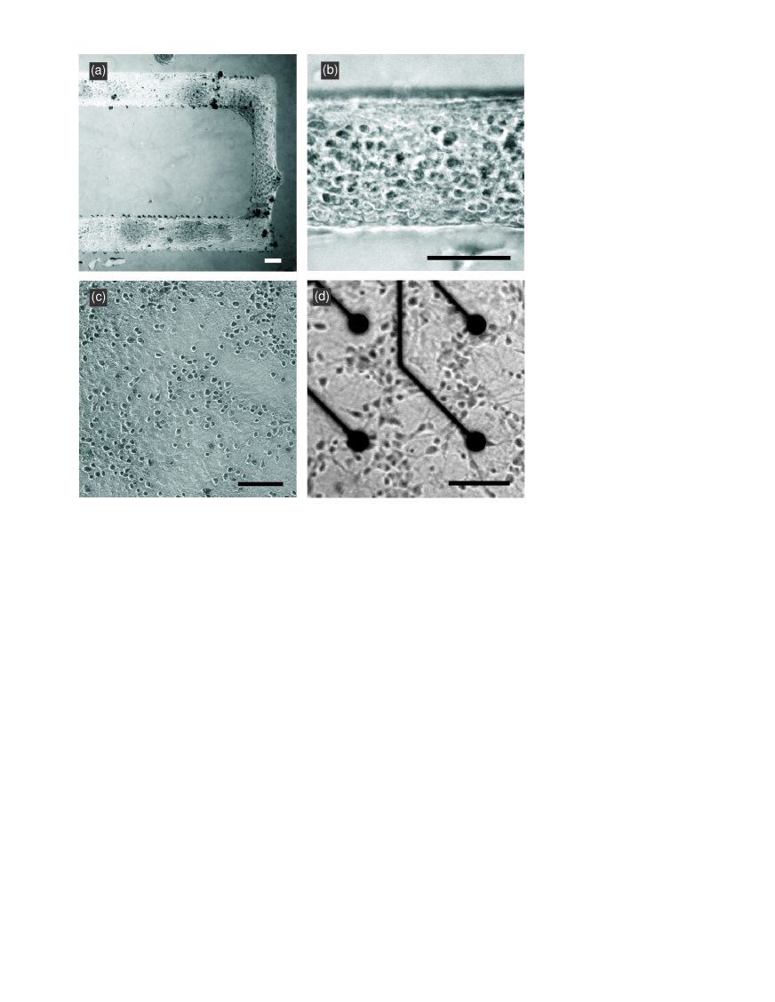
Figure 1: Examples of neural cultures. Dark spots are neurons. (a) Neurons plated in a 1D culture on a pre–patterned line $170$ $\mu$m wide. (b) Detail of the neurons on the line in (a). (c) Neurons plated in a 2D culture on glass coverslips and, (d) multielectrode arrays (MEA), showing the electrodes and the neurons in the area nearby. Scale bars are $100$ $\mu$m.

4 Cell culturing

The history of cell culturing goes back to the end of the 19th and beginning of the 20th century, when Roux and then Harrison showed that cells and neurons can be maintained alive outside of the animal. However, it was not before the 1950’s that immortalization of the cell was achieved by causing a cancer–like bypass of the limitation on the number of its divisions. This enabled the production of cell “lines”, and cultures evolved to become a widespread and accepted research tool. Immortalization was to a large extent irrelevant for neurons, since they do not divide, and reliance on a “primary” culture of neurons extracted directly from the brain remained the norm.

The currently accepted protocol for culturing primary cultures of neurons is well defined and usually involves the dissection of brains from young rats, either embryonic or neo–natal. Cultures are typically prepared from neurons of specific regions of the brain, such as the hippocampus or cortex, dissociated, and plated over glass. Neurons start to develop connections within hours and already show activity $3-4$ days after plating [10]. Experiments are normally carried out at day $14-21$, when the network is fully mature. A complete and detailed description of the culturing process can be found for example in [11, 12, 13]. The culturing process is reproducible and versatile enough to permit the study of neural cultures in a variety of geometries or configurations, and with a broad spectrum of experimental tools (Fig. 1). Modern techniques permit to maintain neural cultures healthy for several months [14, 15], making them excellent model systems to study development [10, 16], adaptation [17, 18], and long–term learning [15, 16, 19, 20, 21] and plasticity [22, 23].

5 Experimental approaches

In this section we review several experimental approaches to study neural cultures, emphasizing those techniques that have been used in our research. We start with the now classical patch–clamp technique, and then describe novel techniques that are adapted to questions which arise naturally when biological systems are considered from a physicists point of view. Such experimental systems are specifically capable of supplying information on the activity of many neurons at once. We give here a brief summary of the advantages and limitations of each of these techniques.

5.1 Patch-clamp

Patch–clamp is a technique that allows the recording of single ion–channel currents or the related changes in cells’ membrane potentials [24, 25]. The experimental procedure consists of attaching a micropipette to a single cell membrane, and it is also possible to put the micropipette in contact with the intracellular medium. A metal electrode placed inside the micropipette reads any small changes in current or voltage in the cell. Data is then amplified and processed with electronics.

The advantage and interest of the patch–clamp technique is that it allows to carry out accurate measurements of voltage changes in the neurons under different physiological conditions. Patch–clamp is one of the major tools for modern neuroscience and drug research [26, 27], and it is in a continuous state of improvement and development. Current techniques allow to study up to $12$ neurons simultaneously, which is an impressive achievement given the difficulty of the accurate placement of the micropipettes and the measurement of the quite weak electrical signals. Remarkable progress has been attained with the development of chip–based patch–clamp techniques [28], where silicon micromachining or micromolding is used instead of glass pipettes. In general, however, given the sophistication of the equipment that patch–clamp requires, measurement of substantially larger number of neurons are not feasible at this point.

As we will see below, techniques addressing many more neurons exist, but they do not reach the precision of the patch–clamp technique.

5.2 Fluorescence and calcium imaging

Fluorescence imaging using fluorescent dyes can effectively measure the change in electric potential on the membrane of a firing neuron (“voltage sensitive dyes”), or the calcium increase that occurs as a consequence (“calcium imaging”) [29, 30]. After incubation with the fluorescent dye, it is possible to measure for a few hours in a fluorescent microscope the activity in the whole field of view of the objective. In our experiments [6], this sample can cover on the order of 600 neurons. Since the culture typically includes $10^{5}$ neurons, this sample represents the square root of the whole ensemble, and should give a good estimation for the statistics of the network.

The response of calcium imaging fluorescence is typically a fast rise (on the order of a millisecond) once the neuron fires, followed by a much slower decay (typically a second) of the signal. This is because the influx of calcium occurs through rapidly responding voltage gated ion channels, while a slower pumping process governs the outflow. This means that the first spike in a train can be recognized easily, but the subsequent ones may be harder to identify. In our measurements we find that the bursting activity characteristic of the network rarely invokes more than five spikes in each neuron, and within this range the fluorescence intensity is more or less proportional to the number of spikes.

The advantages of the fluorescence technique are the ease of application and the possibility of using imaging for the detection of activity, the fast response and the large field of view. It also benefits from continuous advances in imaging, such as the two–photon microscopy [31], which substantially increases depth penetration and sensitivity, allowing the simultaneous monitoring of thousands of neurons. The disadvantages are that the neurons are chemically affected, and after a few hours of measurement (typically $4-6$) they will slowly lose their activity and will eventually die. Subtle changes in their firing behavior may also occur as a result of the chemical intervention.

5.3 Multielectrode arrays (MEA)

Placing numerous metal electrodes on the substrate on which the neurons grow is a natural extension of the single electrode measurement. Two directions have evolved, with very different philosophies. An effort pioneered by the Pine group [32, 33, 34], and represented by the strong effort of the Fromherz group [35, 36, 37], places specific single neurons on top of a measuring electrode. Since neurons tend to connect with each other, much effort is devoted to keep them on the electrode where their activity can be measured, for example by building a “cage” that fences the neurons in. This allows very accurate and precise measurements of the activity, but is highly demanding and allows only a limited number of neurons to be measured.

The second approach lays down an array of electrodes (MEA) on the glass substrate, and the neurons are then seeded on the glass. Neurons do not necessarily attach on the electrodes, they are rather randomly located in various proximities to the electrodes (Fig. 1d). The electrode will in general pick up the signal of a number of neurons, and some spike sorting is needed to separate out activity from the different neurons. The different relative distance of the neurons to the electrodes creates different electric signatures at the electrodes allowing efficient sorting, usually implemented by a simple clustering algorithm.

This approach, originating with the work of Gross [38, 39], has developed into a sophisticated, commercially available technology with ready-made electrode arrays of different sizes and full electronic access and amplification equipment [15, 40, 41, 42]. Electrode arrays typically include $64$ electrodes, some of which can also be used to stimulate the culture. Spacing between the electrodes can vary, but is generally on the order of a few hundred $\mu$m’s.

The advantages of the MEA are the precise measurement of the electric signal, the fast response and high temporal resolution. A huge amount of data is created in a short time, and with sophisticated analysis programs, a very detailed picture can be obtained on the activity of the network. This technique is thus extensively used to study a wide range of problems in neuroscience, from network development to learning and memory [10, 15, 17, 18, 19, 20, 21, 22, 23] and drug development [43, 44]. The disadvantages of the MEA are that the neurons are dispersed randomly, and some electrodes may not cover much activity. The measured extracellular potential signal is low, on the order of several $\mu$V, and if some neurons are located at marginal distances from the electrode, their spikes may be measured correctly at some times and masked by the noise at others.

The lack of accurate matching between the position of the neurons and the one of the microelectrodes may be critical in those experiments where the identification of the spiking neurons is important. Hence, new techniques have been introduced in the last years to enhance the neuron–to–electrode interfacing. Some of the most important techniques are the neural growth guidance and cell immobilization [34, 35, 45, 46]. These techniques, however, have proven challenging and are still far from being standard.

MEA is also limited to the study of the response of single neurons, and cannot deal with collective cell behavior. Phenomena that take place at large scale and involve a huge amount of neurons, such as network structure and connectivity, can not be studied in depth with MEA techniques. This motivated the development of new techniques to simultaneously excite a large region of a neural network and study its behavior. However, methods for excitation of a large number of neurons often lack the recording capabilities of MEA. In addition, these techniques normally use calcium imaging to detect neuronal activity, which shortens drastically the duration of the experiments from days to hours.

An innovative technique, in the middle between MEA and collective excitation, consists on the use of light–directed electrical stimulation of neurons cultured on silicon wafers [47, 48]. The combination of an electric current applied to the silicon surface together with a laser pulse creates a transient “electrode” at a particular location on the silicon surface, and by redirecting the location of the laser pulse it is possible to create complex spatiotemporal patterns in the culture.

5.4 Collective stimulation through bath electrodes

Collective stimulation can be achieved by either electric or magnetic fields applied to the whole culture. Magnetic stimulation techniques for neural cultures are still under development, although they have been successfully applied to locally excite neurons in the brain [49, 50]. Electrical stimulation is becoming a more common technique, particularly thanks to its relative low cost and simplicity. Reiher et al. [51] introduced a planar Ti–Au–electrode interface consisting on a pair of Ti–Au electrodes deposited on glass coverslips and separated by $0.3$ mm. Neurons were plated on the coverslips and were collectively stimulated through the electrodes. Neural activity was measured through calcium–imaging.

Our experiments use both chemical [4] and electric stimulation [6]. The electric version is a variation of the above described technique. Neurons are excited by a global electrical stimulation applied to the entire network through a pair of Pt–bath–electrodes separated by $15$ mm, with the coverslip containing the neural culture centered between them. Neural activity is measured with calcium–imaging.

The major advantage of collective stimulation is that it permits to simultaneously excite and study the response of a large neural population, on the order of $600$ neurons in our experiments [6]. The major disadvantage is that calcium–imaging limits the duration of the experiments, and that repeated excitations at very high voltages ($\gtrsim 10$ V) significantly damage the cells and modify their behavior [51].

6 The activity repertoire of neuronal cultures

When successfully kept alive in culture, neurons start to release signaling molecules, called neurotransmitters, into the environment around them, supposedly intended to attract connections from their neighbors [52, 53]. They also grow long, thin extensions called axons and dendrites that communicate with these neighbors, in order to transmit (axons) or receive (dendrites) chemical messages. At the meeting point between an axon and a dendrite there is a tiny gap, about $200-400$ nm wide, called a chemical synapse. At the dendritic (receiving) side of the synaptic gap there are specialized receptors that can bind the neurotransmitters released from the axon and pass the chemical signal to the other side of the gap. The effect of the message can be either excitatory, meaning that it activates the neuron that receives the signal, inhibitory, i.e., it de–activates the target neuron, or modulatory, in which case the effect is usually more prolonged and complex. The release of neurotransmitters into the synapse is usually effected by a short ($\approx 3$ msec) electrical pulse, called action potential or spike, that starts from the body of the neuron and passes throughout the axon. The neuron is then said to have fired a spike, whose effect on neighboring neurons is determined by the strengths of the synapses that couple them together.

As the cultured neurons grow and connect with each other, they form a network of coupled cells, whose firing activity usually takes one of three main forms: (i) Asynchronous firing (Fig. 2a). Neurons fire spikes or bursts in an uncoordinated manner. This typically occurs at very early developmental stages (e.g., $2-5$ days in vitro  ) or in special recording media [54]. (ii) Network bursts (Figs. 2b-d). This is by far the most common pattern of activity, where short bursts of intense activity are separated by long periods of near–quiescence. (iii) Seizure–like activity. This is an epilepsy–like phenomenon, characterized by very long (tens of seconds) episodes of intense synchronized firing, that are not observed in neuronal cultures under standard growth conditions [55].

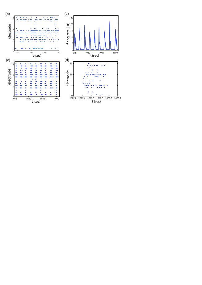
Figure 2: Activity repertoire of neuronal cultures: (a) Raster plot of asynchronous firing, showing time on the x axis and electrode number on the y axis. (b) Network burst, showing the average firing rate across the culture as a function of time. (c) Raster plot of burst activity. Bursts appear as simultaneous activity in nearly all electrodes, separated by silent periods. (d) Zooming in one burst in (c) shows that there is an internal spiking dynamics inside the burst. Data taken from a multielectrode array recording by E. Cohen from hippocampal cultures at the M. Segal lab.

6.1 Network bursts

Fig.  2 shows an example of a network burst, which is a prominent property of many neuronal cultures in vitro  [56, 57]. Several days after plating, cultured neurons originating from various tissues from the central nervous system display an activity pattern of short bursts of activity, separated by long periods of near–quiescence (called inter–burst–interval). This kind of activity persists as long as the culture is maintained [57, 58, 59].

Network bursts also occur in organotypic slices grown in vitro  [60, 61]. Similar patterns of spontaneous activity were found in vivo  in brains of developing embryos [60] and in the cortex of deeply anesthetized animals [62]. Recent evidence suggests that they may also occur in the hippocampus of awake rats during rest periods after intensive exploration activity [63] (called “sharp waves”), as well as during non–REM sleep [64]. Network bursting has been produced experimentally already in the 50’s in cortical “slabs” in vivo  (small areas of the cortex, whose neuronal connections with the rest of the brain are cut, while blood supply is maintained intact [65, 66]). After the surgery the animals recover, but within a few days the slab typically develops network bursts.

These varied physiological states are all characterized by the absence, or a prolonged reduction, in sensory input. Recent modeling and experimental work suggests that low levels of input may indeed be a requirement for network bursting [54, 67, 68, 69], along with a strong–enough coupling between the neurons [70]. Interestingly, bursting appears to be much more sensitive to the background level of input than to the degree of coupling. During periods of low activity, neurons seem to accumulate a large pool of excitable resources. When a large enough group of these “loaded” neurons happens to fire synchronously, they start a fast positive–feedback loop that excites their neighbors and can potentially activate nearly all the neurons in the culture within a short and intense period. Subsequently, the neurons start a long process of recovering the depleted resources until the next burst is triggered.

Modeling studies suggest that when the input to the neurons is strong enough, significant sporadic firing activity occurs during the inter–burst phase and depletes the pool of excitable resources needed to ignite a burst, and thus the neurons fire asynchronously. On the other hand, prolonged input deprivation (e.g., in cortical slabs immediately post-surgery) appears to cause a homeostatic process in which neurons gradually increase their excitability and mutual coupling. Both changes increase the probability of firing action potentials, but in different ways: Increasing excitability can cause neurons to be spontaneously active independently of their neighbors, i.e., in an asynchronous manner, while stronger coupling promotes synchronization. For an unknown reason, under physiological conditions the mutual coupling seems to be increased much more than the individual excitability, and after a few days the neuronal tissue starts bursting.

6.2 Epileptiform activity

In addition to having a yet–unknown physiological significance, network bursts may potentially serve as a toy model for studying mechanisms of synchronization in epilepsy. One of the in vitro  models for epilepsy is seizure-like activity, a phenomenon characterized by very long (tens of seconds) periods of high–frequency firing. It is typically observed either in whole brains [71], in very large cortical slabs [66], or when using certain pharmacological protocols in vitro  [55]. While network bursts are much shorter than seizure–like activity, some experimental and theoretical evidences indicate that when the density and size of a neuronal ensemble is increased, network bursts are replaced by prolonged seizure–like activity [66, 68]. The question of why neuronal ensemble size affects bursting is still being debated, and non-synaptic interactions in the densely–packed tissue of neurons and glia in the brain possibly play an important role, e.g., through regulation of the extracellular $K^{+}$ concentration [72, 73].

6.3 MEA and Learning

In the context of cultures, one can speak of learning in the sense of a persistent change in the way neuronal activity reacts to a certain external stimulus. It is widely believed that the strength of the coupling between two neurons changes according to the intensity and relative timing of their firing. For a physicist, this suggests that neuronal preparations have the intriguing property that the coupling term used in neuronal population modeling is often not constant, but rather changes according to the activity of the coupled systems. The correlation between synchronized firing and changes in coupling strength is known in neurobiology as Hebb’s rule [74, 75].

The typical experiment consists of electrically stimulating groups of neurons with various patterns of “simulated action potentials” and observing the electrical and morphological changes in the cultured neural networks, sometimes called “neuronal plasticity”. These cellular and network modifications may indicate how neurons in living brains change when we learn something new. They may involve changes in the electrical or chemical properties of neurons, in synapse number or size, outgrowth or pruning of dendritic and axonal arbors, formation of dendritic spines, or perhaps even interactions with glial cells.

An interesting approach worth noting is that of Shahaf and Marom [19], who stimulated the network through a single MEA electrode (the input), and measured the response at a specific, different site on the electrode array (the output) within a short time window after stimulation. If the response rate of the output electrode satisfied some predetermined requirement, stimulation was stopped for a while, and otherwise another round of stimulation was initiated. With time, the network “learned” to respond to the stimulus by activating the output electrode. One interpretation of these results is that each stimulation, as it causes a reverberating wave of activity through the network, changes the strengths of the coupling between the neurons. Thus, the coupling keeps changing until the network happens to react in the desired way, at which point stimulation stops and hence the coupling strengths stop changing.

It is perhaps interesting to note that with time, the network seems to “forget” what it learned: spontaneous activity (network bursts that occur without prior stimulation) is believed to cause further modifications in the coupling strengths and a new wiring pattern is formed, a phenomenon reproduced by recent modeling work [76].

Other studies have tried to couple neuronal cultures to external devices, creating hybrid systems that are capable of interacting with the external world [20, 77, 78], for instance to control the movement of a robotic arm [77]. In these systems, input is usually applied through electrodes, and neurons send an output signal in the form of a network burst. Still, more modeling work is needed before it would be possible to use bursts as intelligent control signals for real–world applications. Even though they are so commonly seen and intuitively understood, a true model that can, for instance, forecast the timing of network bursts in advance is still not available.

7 1-D neural cultures

Since we are interested in studying cultures with many neurons, it is natural to look for simplifying experimental designs. Such a simplification can be obtained by constraining the layout of the neurons in the coverslip. Here we focus on the simplest topology of uni–dimensional networks [4, 79, 80, 81], while in the next section we address two–dimensional configurations.

The main advantage of the $1$–D architecture is that, to a first approximation, the probability of two neurons to make a functional connection depends only on a single parameter, namely their distance. A further simplification is introduced by using long lines, since then the connection probability—sometimes referred to as connectivity footprint [82]—falls to zero on a scale much shorter than the length of the culture, and thus it may be considered local. These two simplifications allow one to obtain interesting results even though the study of one–dimensional neural systems is a relatively young field.

Uni–dimensional networks may be regarded as information transmission lines. In this review, we focus on two types of results, the propagation of information and the study of the speed of propagating fronts. In these cases there is good agreement between theory and experiments, which establishes for the first time measurable comparisons between models of collective dynamics and the actual measured behavior of neural cultures.

7.1 Experimental technique

The idea of plating dissociated neurons in confined, quasi one–dimensional patterns was introduced by Maeda et al. [79]. Chang et al. [80] and Segev et al. [81] used pre–patterned lines and photolithographic techniques to study the behavior of $1$–D neural networks with MEA recording. Here we focus on a new technique recently introduced by Feinerman et al. [4, 5]. It consists of plating neurons on pre–patterned coverslips, where only designated lines (usually $170$ $\mu$m wide and up to $8$ cm long) are amenable to cell adhesion. The neurons adhere to the lines and develop processes (axons and dendrites) that are constrained to the patterned line and align along it to form functional connections. The thickness of the line is larger than the neuronal body (soma), allowing a few cells to be located along this small dimension. This does not prevent the network from being one–dimensional since the probability of two cells to connect depends only on the distance between them along the line (but not on direction). On average, a neuron will connect only to neurons that are located no more than $300-400$ $\mu$m from it. Neuronal activity is measured using fluorescence calcium imaging, as described in Sec. 5.2.

7.2 Transmission of information

Activity patterns are used by brains to represent the surroundings and react to them. The complicated behavioral patterns (e.g. [83]) as well as the impressive efficiency (e.g. [84, 85, 86]) of nervous systems prove them to be remarkable for information handling, for communication and as processing systems. Information theory [87, 88] provides a suitable mathematical structure for quantifying properties of transmission lines. In particular, it can be used to assess the amount of information that neural responses carry about the outside world [86, 89, 90, 91, 92, 93]. An analog of this on the one–dimensional culture would be in measuring how much of information injected at one end of the line actually makes it to the other end [5].

Information transmission rates through our one–dimensional systems have little dependence on conduction speed. Rather, efficient communication relies on a substantial variety of possible messages and a coding scheme that could minimize the effects of transmission noise. Efficient information coding schemes in one-dimensional neuronal networks are at the center of a heated debate in the neuroscience community. Patterned neuronal cultures can be used to help verify and distinguish between the contradicting models.

The Calcium imaging we used allows for the measurement of fluorescent amplitudes in different areas across the culture. Amplitudes in single areas fluctuate with a typical variation of $\pm 20\%$ between different bursts. The measured amplitudes are linearly related to the population spiking rate (rate code), which averages the activity over groups of about $100$ neurons and a time window of about $100$ milliseconds. This experimental constraint is not essential and may be bypassed by using other forms of recording (for example linear patterns on MEA dishes [94]), but it is useful in allowing the direct evaluation of the stability of ‘rate coded’ information as it is transmitted across the culture.

The amplitude of the fluorescence signal progresses between neighboring groups of neurons with unity gain. This means, for example, that if the stimulated or ‘input’ area produces a burst with fluorescence that is $10\%$ over its average event, the neighboring area will tend to react the same $10\%$ over its average. However, there is noise in the transmission. This noise becomes more dominant as the ‘input’ and ‘output’ areas are further spaced. In fact, information can be transmitted between two areas but decreases rapidly with the distance. Almost no information passes between areas which are separated by more than ten average axonal lengths (about $4$ mm).

We modeled the decay of information along the one–dimensional culture by a Gaussian relay channel [5]. In this model, the chain is composed of a series of Gaussian information channels (with unity gain in this case) where the output of the $n$th channel acts as input for the $(n+1)$th one. The information capacity of the Gaussian chain is related to that of a single channel. This, in turn, depends only on its signal to noise ratio (SNR).

To check this relation, the average SNR of a channel of a given length was measured in the in vitro  system and this value used to estimate the mutual information between areas spaced at an arbitrary distance. The model produced an excellent quantitative fit to the experimental results without any adjustable parameters. From this it was concluded that rate coded information that is transmitted along the line decays only due to accumulating transmission noise [5].

It should be noted that classical correlation analysis is able to reveal only partially the structures discovered by information theory. The reason is that information theory allows an accurate comparison between information that is being carried in what may be very different aspects of the same signal (e.g., rate and temporal coding schemes as discussed below) [95].

By externally stimulating uni–dimensional cultures at a single point we produced varied responses that can be considered as different inputs into a transmission line. Spontaneous activity also supplies a varied activity at one edge. The stimulated activity then spreads across the culture by means of synaptic interaction to indirectly excite distant parts of it (considered as outputs). At the ‘output’, again, there is a variation of possible responses. Predicting the ‘output’ activity using the pre-knowledge of the ‘input’ activity is a means of evaluating the transmission reliability in the linear culture and may be quantitatively evaluated by estimating the mutual information between the activities of the two areas.

The activity of inhibitory neurons in the culture may be blocked by using neurotransmitter receptor antagonists, leaving a fully excitatory network. Following this treatment, event amplitudes as well as propagation speeds sharply increase. Information transmission, on the other hand, goes down and almost no information passes even between areas which are separated by just a single axonal length. This follows directly from the fact that unity gain between areas is lost, probably because areas react with maximal activity to any minimal input. Thus, we can conclude that the regulation provided by the inhibitory network is necessary for maintaining the stability of the propagating signals.

7.2.1 Further perspectives for temporal codes and rate codes

A similar study was reported in two–dimensional cultures by Beggs et al. [96]. In that study it was concluded that transmission of rate code depends on an excitatory/inhibitory balance that is present in the undisturbed culture. The importance of such a balance for reliable information transmission was also discussed in [96, 97, 98]. Beggs et al. used two–dimensional cultures and numerical simulations to measure distributions of the fraction of the total number of neurons that participate in different events [96]. They show that this distribution exhibits a power law behavior typical of avalanche size distribution that is theoretically predicted for a critical branching process. This criticality is analogous to the unity gain measured on the one–dimensional culture. They suggest that this implies that the natural state of the culture, in which information transmission is maximized, is achieved by self organized criticality [99].

There are two main hypotheses for cortical information representation [100, 101]. The independent coding hypothesis suggests that information is redundantly encoded in the response of single, independent neurons in a larger population. Retrieval of reliable messages from noisy, error prone, neurons may be achieved by averaging or pooling activity over a population or a time window. The coordinated coding hypothesis, on the other hand, suggests that information is not carried by single neurons. Rather, information is encoded, in the exact time lags between individual spikes in groups of neurons.

Theoretical models of information transmission through linear arrays of neurons suggest different coding solutions that fall into the framework of the two hypotheses presented above. Shadlen et al. [98, 102] argue that the firing rate, as averaged over a population of independent neurons over a time window of about $100$ milliseconds, is the efficient means of transmitting information through a linear network. The averaging compensates for noise that is bound to accumulate as the signal transverses through successive groups of neurons. This independent coding scheme is referred to as rate coding. Some studies, however, convey the opposite view [103, 104, 105]. They show that as signals propagate along a one–dimensional array of neurons, the spiking times of neighboring neurons tend to synchronize and develop large scale correlations, entering what is called synfire propagation [106]. The advantages of averaging diminish as populations become correlated and this causes firing rates to approach a predetermined fixed point as the signal progresses. This fixed point has little dependence on the initial firing rate so that all information coded in this rate is lost. The synchronization between neurons does allow, however, the transmission of very precise spiking patterns through which information could reliably be transmitted. This coordinated coding scheme is termed temporal coding [101]. The controversy between these two points of view, which touches on the central question of how the brain represents information, is far from being resolved.

Many information transmission models concentrate on uni–dimensional neuronal networks, not only because of their simplicity, but also for their relation with living neural networks. The cerebral cortex (the part of the brain responsible for transmitting and processing sensory and motor information) is organized as a net of radial linear columns [107, 108, 109]. This fact supplies an important motivation for generating 1–D models for information transmission [105, 108].

Another known in vivo  linear system is the lateral spinothalamic pathway, which passes rate coded sensory information from our fingers to our central nervous system (higher rates correspond to stronger mechanical stimulation). This linear network uses very long axons and only two synaptic jumps to relay the spike rate information. The necessity for such an architecture can be explained by our results for the one–dimensional cultures [5]. This is a clear case in which comparison to the 2D culture and the living brain provides a new perspective: controlling connectivity can simplify networks and also serve as an in vitro  model of in vivo  architectures. This perspective provides novel possibilities by which cultured neurons can be used to study the brain.

7.3 Parallel information channels

Using our patterning techniques one can study more complex architectures to address specific questions. Here we describe an experiment that asks about the information transmission capacity of two parallel thin lines and its relation to their individual capacities.

Two thick areas connected by two thin 80 $\mu$m channels were patterned (Fig. 3a). The average mutual information between the two furthest areas on the line (connected by two alternative routes one $2.6$ mm and the other $3.2$ mm long) is $0.59\pm 0.09$ bits as averaged over $386$ events in $11$ experiments. This is the same as the information measured between two areas at the same distance connected by a single $170$ $\mu$m thick line [5]. In the next part of the experiment, each channel was separately blocked and reopened using concentric pipettes [110] loaded with a spike preventing drug ($0.3$ $\mu$M of TTX) (Fig. 3b). The entropy in the two areas remained roughly the same (within 10%) throughout the experiment, but the mutual information between them changed in accordance with the application of TTX. As each channel is blocked the activity between the areas remains coordinated (Fig. 3b) but mutual information between the burst amplitudes goes down. Once TTX application is halted, the information increases again (although to a value less than the original one by $20-25\%$, which may be indicating that recovery after long periods of TTX application is not full) (Fig. 3c).

Our measurements on the parallel channels supplement the results of the previous subsection. Since it is the spike rate (i.e., the amplitude of the signal) that carries the information rather than the time between bursts, we can conclude that cooperation between the channels is crucial for information transmission. Indeed, when both channels are active, information transmission is enabled, with the same value as measured for a single thick channel. This can be used to understand the nature of the code. For example, specific temporal patterns would have been destroyed as the signal splits to two channels due to the different traversal times and we can conclude that they are not crucial (as anticipated) for passing rate codes.

It would be interesting in the future to use this approach and architecture to investigate other coding schemes.

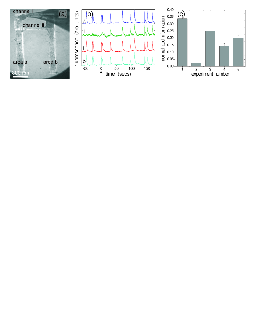
Figure 3: Information capacity of two parallel channels. (a) Two thick areas ($170$ $\mu$m wide) $a$ and $b$ are connected via two thin channels ($80$ $\mu$m wide), labeled $i$ and $ii$. In this image, the concentric pipette, loaded with TTX, is in position to block channel $i$, leaving channel $ii$ open. (b) Fluorescence levels of areas $a$ and $b$, and channels $i$ and $ii$. TTX is applied until time $t=0$ (arrow). During TTX application, channel $i$ is blocked (no signal), while areas $a$ and $b$, and channel $ii$ are co–active. At $t>0$, TTX application is ceased and all four areas return to be simultaneously active. (c) Mutual information between areas $a$ and $b$ normalized by their average entropy [5]. The experiment number corresponds to: 1) both channels open; 2) channel $i$ is blocked; 3) both channels open again; 4) channel $ii$ is blocked; and 5) both channels open.

7.4 Speed of propagating fronts

The next set of experiments deals with measuring causal progression of activity along one–dimensional networks, and comparing it with models of wave propagation. Speed measurements were preformed by Maeda et al. [79] on semi one–dimensional cultures, and by Feinerman et al. [4] for one–dimensional ones.

The uni–dimensional culture displays population activity—monitored using the calcium sensitive dye Fluo4—which commences at localized areas (either by stimulation or spontaneously) and propagates to excite the full length of the line. This should be contrasted with two–dimensional cultures, where front instabilities prevent a reliable measurement of front propagation [111, 112].

The progressing activity front was tracked and two different regimes were identified. Near the point of initiation, up to a few mean axonal lengths, the activity has low amplitude and propagates slowly, at a speed of a few millimeters per second. Activity then either decays or gains both in amplitude and speed, which rises up to $50-100$ mm/s, and stably travels along the whole culture. Similar behavior has been observed in brain slice preparations [113]. The speed of the high amplitude mode can be controlled by modifying the synaptic coupling strength between the neurons [4, 5].

The appearance of two speeds can be understood in terms of an “integrate and fire” (IF) model [3, 114]. The IF model is a minimal model in which neurons are represented by leaky capacitors [115], which fire when their membrane potential exceeds a certain threshold. The time evolution of the membrane potential $u(t)$ is described by

$$\tau\frac{du(t)}{dt}=-u(t)+\sum_{\text{synapses}}\sum_{i=1}^{N}g_{\text{syn}}\;\alpha\left(t-t_{f}^{i}\right),$$ (1)

where $\tau$ is the membrane time constant. The sum above represents the currents injected into a neuron, arriving from $N$ spikes. The synaptic strengths are labeled $g_{\text{syn}}$, and $\alpha(t-t_{f}^{i})$ represents the low–pass filtered synaptic response to a presynaptic spike which fired at time $t_{f}^{i}$. As the voltage across the capacitor exceeds a predefined ‘threshold potential’, the IF neuron ‘spikes’, an event that is modeled as subsequent current injection into its postsynaptic neurons. The voltage on the IF neuron is then reset to a voltage that is lower than the threshold potential.

Continuous versions of the IF model were introduced in [3, 114, 116] by defining a potential $u(x,t)$ for every point $x$ along a single dimension. The connectivity between neurons, $J(|y-x|)$, depends on their distance only, and falls off with some relevant length scale (e.g., the average axonal length). The model incorporates a single synapse type with time constant $\tau_{\rm syn}$. The system is then described by

$$\tau\frac{\partial u(x,t)}{\partial t}=-u(x,t)+\int{J\left(|y-x|\right.)}\sum g_{\text{syn}}\;\exp\bigl{(}{-\frac{t-t_{f}^{i}}{\tau_{\text{syn}}}}\bigr{)}\;H\left(t-t_{f}^{i}\right)\;dy~{},$$ (2)

where $H(t)$ is the Heaviside step function and the sum is, again, over all spikes in all synapses.

In [4], the model was simplified by assuming $N=1$. In this case the wavefront may be fully analyzed in the linear regime that precedes the actual activity front of spiking cells. This model can be analytically solved and predicts two speeds for waves traveling across the system: a fast, stable wave and a slow, unstable one. As the synaptic strength is weakened, the fast speed decreases drastically, while the slower one gradually increases until there is breakup of propagation at the meeting point of the two branches [4]. By introducing into the model the structural data measured on the one–dimensional culture (neuronal density and axonal length distribution), along with the well known single neuron time scales, one observes a strong quantitative agreement between the in vitro  experiment and the theoretical predictions [4].

The two wave speeds can be understood because there are two time scales in the model. The fast wave corresponds to the fast time scale of the synaptic transmission, and is relevant for inputs which coincide at this short scale of a few milliseconds. The slower wave corresponds to the longer membrane leak time constant and involves input activity which is less synchronized. A similar transition from asynchronous to synchronous activity during propagation through a one–dimensional structure was previously predicted by the theoretical model of Diesmann et al. [104]. This transition plays an important role in information transmission capabilities as elaborated below.

7.4.1 Perspectives and implications to other approaches

Richness of the speed of the fast propagating front was also observed in some experiments with brain slices [113, 117]. We found that this fast speed scaled linearly with the amplitude of the excitation, which measures the number of spikes in a propagating burst (Fig. 4) (see also [94]). Larger amplitudes signify more spiking in pre–synaptic cells and may be accounted for through a proper re–scaling of the synaptic strength, $g_{\text{syn}}$. Such re–scaling should take into account the relative synchronicity between spikes as only spikes that are separated by an interval that is less than the membrane time constant can add up. Multiple spike events are more difficult to understand theoretically. Osan et al. [114] expand their one–spike model into two spikes and demonstrate a weak dependence of speeds on spike number. A more comprehensive analysis of traveling waves that includes periodic spiking is introduced in [114, 118] and predicts dispersion relations that may scale between $g_{\text{syn}}^{1/2}$ and $g_{\text{syn}}^{2}$, so that a linear relation is not improbable. Golomb et al. [82] use a simulation of a one–dimensional network composed of Hodgkin–Huxley type model neurons and two types of excitatory synapses (AMPA and NMDA) to find a weak linear relation between propagation speed and the number of spikes in the traveling front.

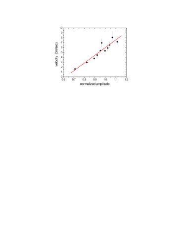
Figure 4: Propagation speed as a function of burst amplitude. The plot summarizes $74$ spontaneous events that travel across a $17$ mm line. Amplitudes naturally vary between bursts (about $\pm 20\%$ around the average normalized value of 1). The amplitude for each event (while the signal travels along the line) is averaged over several areas on the line (the two ends and the central part) [5]. Speed measurements were preformed as described in [4] and are seen to scale linearly with the amplitude.

More complex behavior is predicted by theoretical models of one–dimensional neural networks that incorporate mixed populations of excitatory and inhibitory neurons and different connection footprints. Such networks were shown to support a variety of propagating modes: slow–unstable, fast–stable, and lurching [119, 120]. Similar models include bistable regimes where a fast–stable and a partially slower–stable modes coexist and develop according to specific initial conditions [121, 122].

8 2-D neural cultures

As we have seen, one–dimensional neural cultures allow us to study the speed of propagating fronts, information content and coding schemes. In contrast, two–dimensional neural cultures involve a large neural population in a very complex architecture. Therefore, they are excellent model systems with which to study problems such as connectivity and plasticity, which is the basis for learning and memory.

Abstract neural networks, their connectivity and learning have caught the attention of physicists for many years [123, 124, 125]. The advent of novel experimental techniques and the new awakening of graph theory—with its application to a large variety of fields, from social sciences to genetics—allow one to shed new light on the study of the connectivity in living neural networks.

The study of networks, namely graphs in which the nodes are neurons and the links are connections between neurons, has received recently a vast theoretical input [126, 127, 128]. We are here not so much interested in the scale–free graphs, although they seem omni–present in certain contexts, but rather in the more information-theoretic aspects. These aspects have to do with what we believe must be the main purpose of neurons: to communicate. An admittedly very simple instance of such an approach is the study of the network of e-mail communications [129, 130]. In that case, encouraging results were found, and one can try to transport the insights from those studies to the study of in vitro  neural networks. What they have in common with an e-mail network is the property that both organize without any external master plan, obeying only constraints of space and time.

8.1 Percolation in neural networks

Neurons form complex webs of connections. Dendrites and axons extend, ramify, and form synaptic links with their neighbors. This complex wiring diagram has caught the attention of physicists and biologists for its resemblance to problems of percolation [131, 132]. Important questions are the critical distance that dendrites and axons have to travel in order to make the network percolate, i.e., to establish a path from one neuron of the network to any other, or the number of bonds (connections) or sites (cell bodies) that can be removed without critically damaging the functionality of the circuit. In the brain, neural networks display such robust flexibility that circuits tolerate the destruction of many neurons or connections while keeping the same, though degraded, function. For example, it is currently believed that in Parkinson’s disease, up to $70$% of the functionality of the neurons in the affected areas can be lost before behavioral symptoms appear [133].

One approach that uses the concept of percolation combines experimental data of neural shape and synaptic connectivity [134, 135] with numerical simulations to model the structure of living neural networks [134, 136, 137]. These models are used to study network dynamics, optimal neural circuitry, and the relation between connectivity and function. Despite these efforts, an accurate mapping of real neural circuits, which often show a hierarchical structure and clustered architecture (such as the mammalian cortex [138, 139]), is still unfeasible.

8.2 Bond-percolation model

At the core of our experiments and model [6] is a completely different approach. We consider a simplified model of a neural network in terms of bond–percolation on a graph. The neural network is represented by the directed graph $G$ with the following simplifying assumptions:  A neuron has a probability $f$ to fire in direct response to an external excitation (an applied electrical stimulus in the experiments), and it always fires if any one of its input neurons fire (Fig. 5a).

The fraction of neurons in the network that fire for a given value of $f$ defines the firing probability $\Phi(f)$. $\Phi(f)$ increases with the connectivity of $G$, because any neuron along a directed path of inputs may fire and excite all the neurons downstream (Fig. 5a). All the upstream neurons that can thus excite a certain neuron define its input–cluster or excitation–basin. It is therefore convenient to express the firing probability as the sum over the probabilities $p_{s}$ of a neuron to have an input cluster of size $s-1$ (Fig. 5b),

$$\Phi(f) = f+(1-f)P\left(\mbox{any input neuron fires}\right)$$ (3)

$$= f+(1-f)\sum_{s=1}^{\infty}p_{s}\left(1-\left(1-f\right)^{s-1}\right)=1-\sum_{s=1}^{\infty}p_{s}\left(1-f\right)^{s},$$

with $\sum\nolimits_{s}p_{s}=1$ (probability conservation). The firing probability $\Phi(f)$ increases monotonically with $f$, and ranges between $\Phi(0)=0$ and $\Phi(1)=1$. The connectivity of the network manifests itself by the deviation of $\Phi(f)$ from linearity (for disconnected neurons one has $p_{1}=1$ and $\Phi(f)=f$). Equation (3) indicates that the observed firing probability $\Phi(f)$ is actually one minus the generating function $H(x)$ (or the $z$–transform) of the cluster–size probability $p_{s}$ [140, 141],

$$H(x)=\sum_{s=1}^{\infty}p_{s}x^{s}=1-\Phi(f)~{},$$ (4)

where $x=1-f$. One can extract from $H(x)$ the input–cluster size probabilities $p_{s}$, formally by the inverse $z$–transform, or more practically, in the analysis of experimental data, by fitting $H(x)$ to a polynomial in $x$.

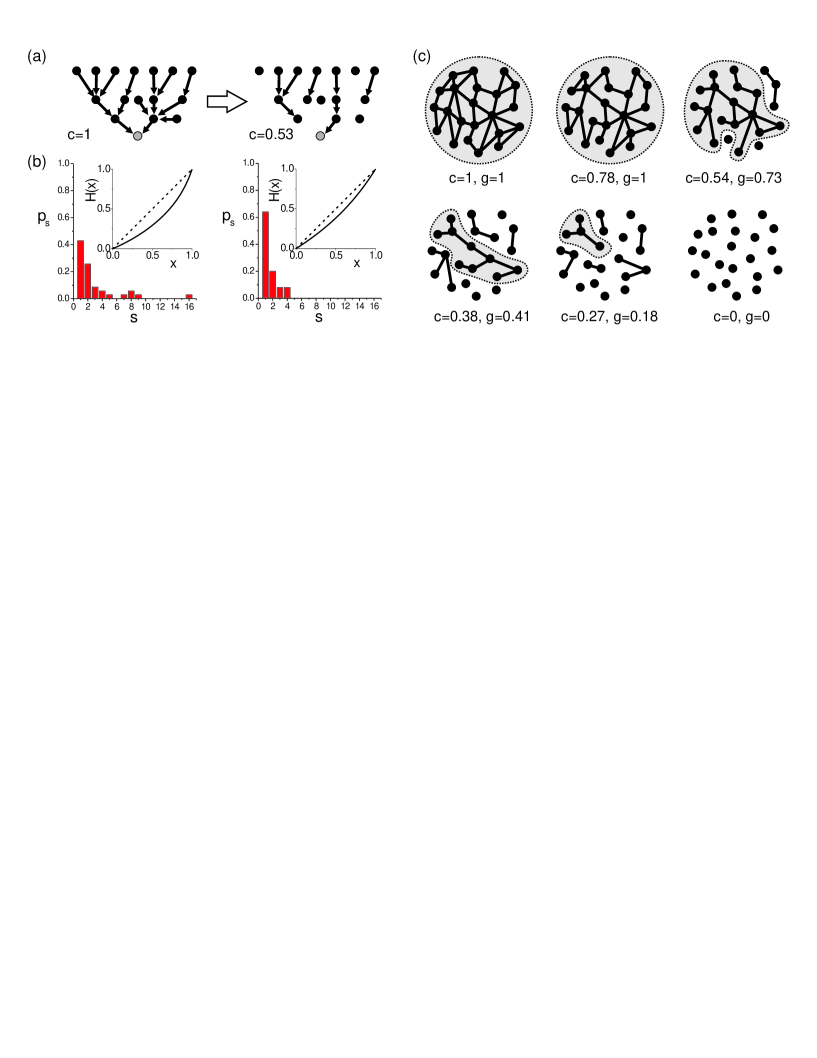
Figure 5: (a) Percolation model. The neuron represented in grey fires either in response to an external excitation or if any of its input neurons fire. At the highest connectivity, this neuron has input clusters of size $s-1=0$ (the neuron responds to the external excitation only), $7$ (left branch), $8$ (right branch), and $15$ (both branches). At lower connectivity, its input–clusters are reduced to sizes $0$ and $3$. (b) Corresponding $p_{s}$ distributions, obtained by counting all input clusters for all neurons. Insets: The functions $H(x)$ (solid lines), compared with those for unconnected neurons (dashed lines). (c) Concept of a giant component: The grey areas outline the size of the giant component $g$ (biggest cluster) for gradually lower connectivity $c$.

In graph theory, say in a random graph, one considers connected components. When the graph has $N$ nodes, one usually talks about a giant (connected) component if, in the limit of $N\to\infty$, the largest component has a size which diverges with $N$ [142]. Once a giant component emerges (Fig. 5c) the observed firing pattern is significantly altered. In an infinite network, the giant component always fires no matter how small the firing probability $f>0$ is. This is because even a very small $f$ is sufficient to excite one of the infinitely many neurons that belong to the giant component. This can be taken into account by splitting the neuron population into a fraction $g$ that belongs to the giant component and always fires and the remaining fraction $1-g$ that belongs to finite clusters (Fig. 5c). This modifies the summation on cluster sizes into

$$\Phi(f) = g+(1-g)\left[f+(1-f)P\left(\mbox{any input neuron fires}\right)\right]$$ (5)

$$= 1-(1-g)\sum_{s=1}^{\infty}p_{s}\left(1-f\right)^{s}.$$

As expected, at the limit of almost no excitation $f\rightarrow 0$ only the giant component fires, $\Phi(0)=g$, and $\Phi(f)$ monotonically increases to $\Phi(1)=1$. With a giant component present the relation between $H(x)$ and the firing probability changes, and Eq. (4) becomes

$$H(x)=\sum_{s=1}^{\infty}p_{s}x^{s}=\frac{1-\Phi(f)}{1-g}.$$ (6)

As illustrated schematically in Fig. 5c, the size of the giant component decreases with the connectivity $c$, defined as the fraction of remaining connections in the network. At a critical connectivity $c_{0}$ the giant component disintegrates and its size is comparable to the average cluster size in the network. This behavior suggests that the connectivity undergoes a percolation transition, from a world of small, disconnected clusters to a fast growing giant cluster that comprises most of the network.

The particular details of the percolation transition, i.e., the value of $c_{0}$ and how fast the giant component increases with connectivity, depend on the degree distribution of the neural network. Together with experiments and numerical simulations, as described next, it is possible to use the percolation model to construct a physical picture of the connectivity in the neural network.

8.3 Joining theory and experiment

In our experiments [6] we consider cultures of rat hippocampal neurons plated on glass coverslips, and study the network response (fluorescence as described earlier) to a collective electric stimulation. The network response $\Phi(V)$ is quantified in terms of the fraction of neurons that respond to the external excitation at voltage $V$. When the network is fully connected, the excitation of a small number of neurons with low firing threshold suffices to light up the entire network. The response curve is then similar to a step function, as shown in Fig. 6a. Gradual weakening of the synaptic strength between neurons, which is achieved by blocking the AMPA–glutamate receptors of excitatory neurons with the antagonist CNQX [6], breaks the network off in small clusters, while a giant cluster still contains most of the neurons. The response curves are then characterized by a sudden jump that corresponds to the giant cluster (or giant component) $g$, and two tails that correspond to clusters of neurons with either small or high firing threshold. At the extreme of full blocking the network is completely disconnected, and the response curve $\Phi_{\infty}(V)$ is characterized by the response of individual neurons. $\Phi_{\infty}(V)$ is well described by an error function $\Phi(V)=0.5+0.5\;\mathrm{erf}\left((V-V_{0})/{\sqrt{2}\,\sigma_{0}}\right)$, indicating that the firing threshold of individual neurons follows a Gaussian distribution with mean $V_{0}$ and width $2\sigma_{0}$.

To study the size of the giant component as a function of the connectivity we consider the parameter $c=1/(1+\text{[CNQX]}/K_{d})$, where $K_{d}$ is the concentration of CNQX at which $50$% of the receptors are blocked [6, 143]. Hence, $c$ quantifies the fraction of receptor molecules that are not bound by the antagonist CNQX and therefore are free to activate the synapse. Thus, $c$ characterizes the connectivity in the network, taking values between $0$ (full blocking) and $1$ (full connectivity).

The size of the giant component $g$ as a function of the connectivity is shown in Fig. 6b. Since neural cultures contain both excitatory and inhibitory neurons, two kind of networks can be studied. $G_{EI}$ networks are those containing both excitatory and inhibitory neurons. $G_{E}$ networks contain excitatory neurons only, with the inhibitory neurons blocked with the antagonist bicuculine. The giant component in both networks decreases with the loss of connectivity in the network, and disintegrates at a critical connectivity $c_{0}$. We study this behavior as a percolation transition, and describe it with the power law $g\sim|1-c/c_{0}|^{\beta}$ at the vicinity of the critical point. Power law fits provide the same value of $\beta=0.65\pm 0.05$ within experimental error (inset of Fig.  6b), suggesting that $\beta$ is an intrinsic property of the network. The giant component for $G_{EI}$ networks breaks down at a lower connectivity (higher concentration of CNQX) than for $G_{E}$ networks, indicating that the role of inhibition is to effectively reduce the number of inputs that a neuron receives on average.

The values of $c_{0}$ for $G_{E}$ and $G_{EI}$ networks, denoted by $c_{e}$ and $c_{ei}$ respectively, with $c_{e}\simeq 0.24$ and $c_{ei}\simeq 0.36$, provide an estimation of the ratio between inhibition and excitation in the network. From percolation theory, $c_{0}\sim 1/n$, with $n$ the average number of connections per neuron. Thus, for $G_{E}$ networks, $c_{e}\sim 1/n_{e}$, while for $G_{EI}$ networks $c_{ei}\sim 1/(n_{e}-n_{i})$ due to the presence of inhibition. The ratio between inhibition and excitation is then given by $n_{i}/n_{e}=1-(c_{e}/c_{ei})$. This provides $75$% excitation and $25$% inhibition in the neural culture, in agreement with the values reported in the literature, which give an estimation of $70-80\%$ excitatory neurons [16, 144].

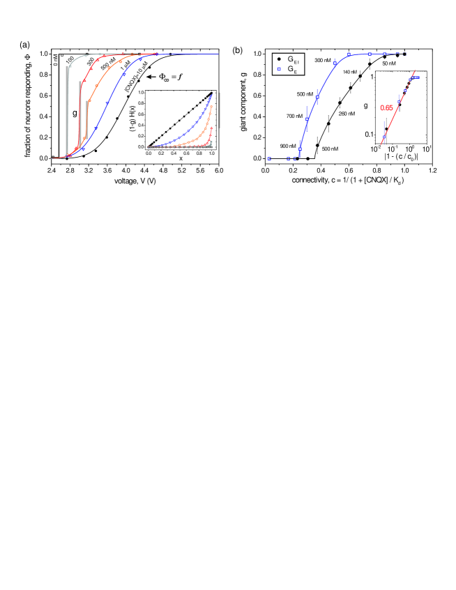
Figure 6: (a) Example of response curves $\Phi(V)$ for 6 concentrations of CNQX. The grey vertical bars show the size of the giant component. They signal large jumps of the number of neurons lighting up, for a small change of voltage. Thin lines are a guide to the eye except for the $1$ $\mu$M and $10$ $\mu$M lines that are fits to error functions. Inset: Corresponding $H(x)$ functions. The bar shows the size of the giant component for $300$ nM. (b) Size of the giant component as a function of the connectivity $c$, for the network containing both excitatory and inhibitory neurons ($G_{EI}$, circles), and a network with excitatory neurons only ($G_{E}$, squares). Lines are a guide to the eye. Some CNQX concentrations are indicated for clarity. Inset: Log–log plot of the power law fits $g\sim|1-c/c_{o}|^{\beta}$. The slope $0.65$ corresponds to the average value of $\beta$ for the two networks. Adapted from I. Breskin, J. Soriano, E. Moses, T. Tlusty, Phys. Rev. Lett. 97, 188102, © 2006 by the American Physical Society.

The response curves $\Phi(V)$ measured experimentally can be analyzed within the framework of the model to extract information about the distribution of input clusters that do not belong to the giant component. Since the response curve for a fully disconnected network characterizes the firing probability $f(V)$ of independent neurons, generating functions $H(x)$ can be constructed by plotting each response curve $\Phi(V)$ as a function of the response curve for independent neurons, $\Phi_{\infty}(V)$, as shown in the inset of Fig. 6a. For those response curves with a giant component present, its contribution is eliminated, and the resulting $H(x)$ function re–scaled with the factor $1-g$, according to Eq. (6). The distribution of input clusters $p_{s}$ is then obtained as the coefficients in the polynomial fits of $H(x)$. Fig. 7a shows the $p_{s}$ distribution for the $\Phi(V)$ curves and $H(x)$ functions shown in Fig 6a.

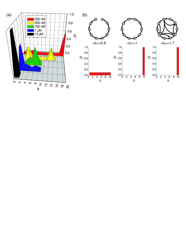
Figure 7: (a) Cluster size distribution $p_{s}$ for the generating functions shown in Fig. 6(a). The values in the table indicate the concentration of CNQX for each curve. (b) Sensitivity of peaks in $p_{s}$ to loops. Left: neurons forming a chain–like connectivity give a $p_{s}$ distributed uniformly. Center: closing the loop by adding just one link collapses $p_{s}$ to a single peak. Right: additional links increase the average connectivity $\langle k\rangle$, but do not modify $p_{s}$. Figure (a) adapted from I. Breskin, J. Soriano, E. Moses, T. Tlusty, Phys. Rev. Lett. 97, 188102, © 2006 by the American Physical Society.

The most remarkable feature of the $p_{s}$ distribution shown in Fig. 7a is that it is characterized by the presence of isolated peaks. These peaks are present even for relatively high concentrations of CNQX (around $500$ nM). The explanation for this observation is that the connectivity in the neural network is not tree–like, but rather characterized by the presence of loops. As illustrated in Fig. 7b, loops alter significantly the distribution of input clusters, collapsing $p_{s}$ to single peaks. This idea is supported experimentally by the observation that the areas of the neural culture with the highest density of neurons tend to fire together in response to the external excitation. Their collective firing is maintained even for high concentrations of CNQX, indicating that neurons may reinforce their connections with close neighbors.

While the analysis of $H(x)$ provides a picture of the distribution of input clusters and the connectivity at a local scale, the analysis of the exponent $\beta$ provides information about the connectivity of the whole network. The exponent $\beta$, and the behavior of the whole $g(c)$ curves shown in Fig. 6b, depend on the actual distribution of connections per node in the network, $p_{k}$. Although the simple percolation model can be extended to derive in principle $p_{k}$ from $H(x)$, the peaked distribution of $p_{s}$ points at limitations of the analysis. Hence, numerical simulations of the model have been explored to elucidate the degree distribution of the neural network. Numerical simulations provide $\beta\simeq 0.66$ for a Gaussian degree distribution, while they give $\beta\geq 1$ when the degree distribution follows a power law [6], and this is clearly different from the experimental observations. In should be kept in mind that the exponents we measure may differ from the critical ones, since we measure them up to values of $c$ that are far from the transition point.

Overall, we conclude that the neural culture can be viewed as a graph with a local connectivity with Gaussian degree distribution and a significant presence of clusters or loops that are maintained even at a low connectivity. Next, we will see how the analysis of the percolation curves $g(c)$ can be used to extract additional information about the connectivity in the neural network.

8.4 Extracting biologically relevant properties from the percolation exponent

In this subsection, we will discuss how to combine mathematical constraints about percolation with experimental observations to draw conclusions about the nature of the network: degree distributions, length of neuronal connections, and the exponent $\beta$.

Two biologically relevant features of the living network arise in relation to the percolation exponent of a random graph model. First, the living network is a directed graph, so that we can make a distinction between the degree distribution of the input graph (dendrites), for which the random graph model gives strong results, and the output graph (axons), for which we can only make reasonable speculations.

Second, since the living network is located in real space, the links have a length associated with them, while the random graph described by purely topological models does not. We will see that the degree distribution is associated with a length distribution.

The input graph degree distribution is Gaussian We want to use the predictions of the random graph model, and compare the measured growth curve of the giant component to what theory predicts for a general random graph [145]. We look at $p_{k}$, the probability that a node has $k$ inputs, make the simplifying assumption that a node fires if any of its inputs fires, and get the firing probability $\Phi(f)$ in terms of $p_{k}$:

$$\Phi(f)=f+(1-f)\sum_{k}p_{k}\left(1-\left(1-\Phi\right)^{k}\right).$$ (7)

with $f(V)$ again the probability of a single neuron to fire at excitation voltage $V$. As usual, one forms the formal power series (or generating function)

$$\widetilde{p}(z)\,=\,\sum_{s=1}^{\infty}p_{k}z^{k}~{}.$$ (8)

The giant component appears already at zero excitation for an infinite size network, we therefore set $f=0$, which practically means that only the giant component lights up, so that $\Phi=g$. From Eq. (8) we find that the probability for no firing, $1-g$, is then a fixed point of the function $\widetilde{p}$

$$1-g=\widetilde{p}(1-g).$$

To proceed we need to know how the generating function is transformed when the edges are diluted to a fraction $c$. It can be shown that it behaves according to $\widetilde{p}(1-g)\rightarrow$ $\widetilde{p}(1-cg)$. Solving now the fixed point equation

$$1-g\,=\,\widetilde{p}(1-cg)$$ (9)

for the fraction $g(c)$ of nodes in the giant component as a function of $c$, we get a correspondence that depends on the edge distribution $p_{k}$.

The strength of this approach is that now the experimentally measured $g(c)$ can be transformed to a result on $p_{k}$. In practice this necessitates some assumptions about $p_{k}$, which can then be tested to see if they fit the experimental data. One popular choice for $p_{k}$ is the scale-free graph, $p_{k}=\mathrm{const}\cdot k^{-\gamma}$. In that case we get

$$1-g=\frac{\text{Li}_{\gamma}(1-cg)}{\zeta(\gamma)},$$ (10)

where Li_γ is the polylogarithmic function and $\zeta(\gamma)$ is the Riemann zeta function. Another frequently studied distribution is the Erdös–Rényi (ER) one, $p_{k}\sim\lambda^{k}/k!$. In this case we obtain

$$g(c)=1+\omega(-\lambda ce^{-\lambda c})/\lambda c,$$ (11)

where Lambert’s $\omega$ is defined as the solution of $x=\omega(x)\exp[\omega(x)]$. A comparison with the curves of Fig. 6b immediately shows that there is a very good fit with Eq. (11), while Eq. (10) shows poor agreement. One can conclude from this that the input graph of neural networks is not scale-free.

Taking space into account The graphs of living neural networks are realized in physical space, in a two-dimensional environment very like a 2D lattice. What is absent in the percolation theory is the notion of distances, or a metric. A seemingly strong constraint therefore is the well-known and amply documented fact, that the exponent $\beta$ in dimension $2$ with short-range connections is $5/36\approx 0.14$ [131]. This is obviously very different from the measured value of about $0.65$.

To study this difficulty, we first observe that long range connections can change the exponent $\beta$. (For the moment, we ignore the fact that long range connections for the input graph have been excluded, since we have shown that the input degree distribution is Gaussian and the dendrites have relatively short length.) Take a lattice in 2 dimensions, for example $\mathbf{Z}^{2}$ and consider the percolation problem on this lattice. Then, there is some critical probability $p_{\mathrm{c}}$ with which links have to be filled for percolation to occur; in fact $p_{\mathrm{c}}=1/2$. There are very precise studies of the behavior for $p>p_{\mathrm{c}}$, and, as said above, in (large) volume $N$ the giant component has size $N(p-p_{\mathrm{c}})^{5/36}$. What we propose is to consider now a somewhat decorated lattice in which links of length $L$ occur with probability proportional to $L^{-s}$, and we would like to determine $s$, knowing the dimension $d=2$ and the exponent $\beta\simeq 0.65$. Like the links of the square lattice, these long links are turned active or inactive with some probability. It is here that we leave the domain of abstract graphs and consider graphs which are basically in the plane. We conjecture that there is a relation between the dimension $d$, the decay rate $s$ and the exponent $\beta$. Results in this direction have been found long ago by relating percolation to the study of Potts models in the limit of $q=1$. For example, it is well-known, and intuitively easy to understand, that if there are too many long range connections, the giant component will be of size $N$ and in fact this is reached for $s\leq d$, see for example [146], which contains also references to earlier work. The variant of the question we have in mind does not seem to have been answered in the literature. If there is indeed a relation between $d$, $\beta$, and $s$, then it can be used to determine $s$ from the experimentally measured values of $\beta$ and will give information about the range of the neural connections.

We now come back to the neural network, keeping in mind that the input connections are short, and have Gaussian distribution. We use the fact that the input and output graphs of the living neural network are different to suggest a way to reconcile an observed Gaussian distribution of input edges and the obvious existence of local connections, with the small exponent of $5/36$ predicted for a locally connected graph in 2D. More specifically, we use the fact that while axons may often travel large distances, the dendritic tree is very limited. We assume that the number of output connections is proportional to the length of the axon. Similarly the number of input connections is proportional to the number of dendrites, to their length and to the density of axons in the range of the dendritic tree.

A possible scenario for long-range connectivity relies therefore on a number of axons that go a long distance $L$. Their abundance may occur with probability proportional to $L^{-s}$, in which case the output graph will have a scale free distribution. However, the input graph may still be Gaussian because there are a finite number of dendrites (of bounded length) and each of them can only accept a bounded number of axons.

Thus, we can conclude the following information about the neural network:

One limitation of using the exponent $\beta$ is the masking of the critical percolation transition by finite size effects and by inherent noise. While the following analysis gives excellent fits with the data, we have to remember that the biological system is not ideal for extracting $\beta$ accurately.

If $\beta$ is indeed the critical exponent, and the graph is not scale-free, then, a change of $\beta$ from the 2-D value can perhaps be explained by assuming that a fixed proportion of neurons extend a maximal distance. This structure will give the necessary long-range connections, but its effect on the distribution of output connections will only be to add a fixed peak at high connectivity. The edge distribution of the input graph will not be affected by such a construction.

While the shortcomings of the discussion will be evident to the reader, we still hope that this shows the important methodological conclusion that, by using theory and experiment together, we are able to put strong constraints on the possible structures of the living neural network.

9 Acknowledgments

We thank M. Segal, I. Breskin, S. Jacobi, and V. Greenberger for fruitful discussions and technical assistance. J. Soriano acknowledges the financial support of the European Training Network PHYNECS, project No. HPRN-CT-2002-00312. J.-P. Eckmann was partially supported by the Fonds National Suisse and by the A. Einstein Minerva Center for Theoretical Physics. This work was also supported by the Israel Science Foundation, grant No. 993/05, and the Minerva Foundation, Munich, Germany.

References

- [1] G. Stent, Phage and the Origins of Molecular Biology, Expanded edition. Cold Spring Harbor Laboratory Press, 1992.
- [2] J.D. Watson, A. Berry, DNA: The Secret of Life. Knopf Ed., 2003.
- [3] R. Osan, B. Ermentrout, Physica D 163 (2002) 217.
- [4] O. Feinerman, M. Segal, E. Moses, J. Neurophysiol. 94 (2005) 3406.
- [5] O. Feinerman, E. Moses, J. Neurosci. 26 (2006) 4526.
- [6] I. Breskin, J. Soriano, E. Moses, T. Tlusty, Phys. Rev. Lett. 97 (2006) 188102.
- [7] K. Nakanishi, F. Kukita, Brain Res. 795 (1998) 137.
- [8] K. Nakanishi, M. Nakanishi, F. Kukita, Brain Res. Protoc. 4 (1999) 105.
- [9] K. Nakanishi, F. Kukita, Brain Res. 863 (2000) 192.
- [10] D. A. Wagenaar, J. Pine, S. M. Potter, BMC Neurosci. 7 (2006) 1.
- [11] M.C. Bundman, V. Greenberger, M. Segal, J. Neurosci. 15 (1995) 1.
- [12] D.D. Murphy, M. Segal, J. Neurosci. 16 (1996) 4059.
- [13] G. Banker, K. Goslin. Culturing Nerve Cells. 2nd Ed. MIT Press, Cambridge, 1998.
- [14] K.V. Gopal, G.W. Gross, Acta oto-lar. 116 (1996) 690.
- [15] S. M. Potter, T. B. DeMarse, J. Neurosci. Methods 100 (2001) 17.
- [16] S. Marom, G. Shahaf, Q. Rev. Biophys. 35 (2002) 63.
- [17] G. Fuhrmann, H. Markham, M. Tsodyks, J. Neurophysiol. 88 (2002) 761.
- [18] M. Giugliano, P. Darbon, M. Arsiero, H.-R. Lüscher, J. Streit, J. Neurophysiol. 92 (2004) 977.
- [19] G. Shahaf, S. Marom, J. Neurosci. 21 (2001) 8782.
- [20] N. DeMarse, D. Wagenaar, A. Blau, S. Potter, Auton. Robots 11 (2001) 305.
- [21] D. Eytan, N. Brenner, S. Marom, J. Neurosci. 23 (2003) 9349.
- [22] E. Maeda, Y. Kuroda, H.P.C. Robinson, A. Kawana, Eur. J. Neurosci. 10 (1998) 488.
- [23] Y. Jimbo, T. Tateno, H.P.C. Robinson, Biophys. J. 76 (1999) 670.
- [24] O.P. Hamill, A. Marty, E. Neher, B. Sakmann, F.J. Sigworth, Pflugers Arch. 391 (1981) 85.
- [25] E. Neher, Neuron 8 (1992) 605.
- [26] D. Owen, A. Silverthorne, Drug Discovery World 3 (2002) 48.
- [27] A. Stett, U. Egert, E. Guenther, F. Hofmann, T. Meyer, W. Nisch, H. Haemmerle, Anal. Bioanal. Chem. 377 (2003) 486.
- [28] C. Ionescu-Zanetti, R. M. Shaw, J. Seo, Y.-N. Jan, L. Y. Jan, and L. P. Lee. Proc. Nat. Acad. Sci. USA 102 (2005) 9112.
- [29] J.P. Kao, Methods Cell Biol. 40 (1994) 155.
- [30] K.R. Gee, K.A. Brown, W.N. Chen, J. Bishop-Stewart, D. Gray, I. Johnson, Cell Calcium 27 (2000) 97.
- [31] O. Garaschuk, J. Linn, J. Eilers, A. Konnerth, Nature Neurosci. 3 (2000) 452.
- [32] J. Pine, J. Neurosci. Methods 2 (1980) 19.
- [33] W.G. Regehr, J. Pine, C.S. Cohan, M.D. Mischke, D.W. Tank, J. Neurosci. Methods 30 (1989) 91.
- [34] M. P. Maher, J. Pine, J. Wright, Y.-C. Tai, J. Neurosci. Meth. 87 (1999) 45.
- [35] G. Zeck, P. Fromherz, Proc. Nat. Acad. Sci. USA 98 (2001) 10457.
- [36] P. Fromherz, in Nanoelectronics and Information Technology, pp. 781-810. Editor R. Waser, Wiley-VCH, Berlin, 2003.
- [37] P. Fromherz, in Bioelectronics from theory to applications, pp. 339-394. Eds. I. Willner & E. Katz, Wiley-VCH, Weinheim, 2005.
- [38] G. Gross, IEEE Trans. Biomed. Eng. 26 (1979) 273.
- [39] G. Gross, B. Rhoades, D. Reust, F. Schwalm, J. Neurosci. Methods 50 (1993) 131.
- [40] Y. Jimbo, A. Kawana. Bioelectrochem. Bioenerget. 29 (1992) 193.
- [41] M. Meister, J. Pine, D.A. Baylor, J. Neurosci. Methods 51 (1994) 95.
- [42] S. M. Potter, D. A. Wagenaar, T. B. DeMarse, in Advances in Network Eletrophysiology Using Multi-Electrode Arrays, pp. 215-242. M. Taketani & M. Baudry (Eds.) Springer, New York, 2006.
- [43] S.I. Morefield, E.W. Keefer, K.D. Chapman, G.W. Gross. Biosens. Bioelectron. 15 (2000) 383.
- [44] A. Stett, C. Burckhardt, U. Weber, P. van Stiphout, T. Knott. Recept. Channels 9 (2003) 59.
- [45] P. Fromherz, H. Schaden, T. Vetter, Neurosci. Lett. 129 (1991) 77.
- [46] N. Sanjana, S. Fuller, J. Neurosci. Methods 136 (2004) 151.
- [47] S. Artem, J. Choi, H.S. Seung, J. Neurophysiol. 93 (2005) 1090.
- [48] M.A. Colicos, B.E. Collins, M.J. Sailor, Y. Goda, Cell 107 (2001) 605.
- [49] M. Hallett, Nature 406 (2000) 147.
- [50] A. Pascual-Leone, V. Walsh, J. Rothwell, Curr. Opin. Neurobiol. 10 (2000) 232.
- [51] A. Reiher, S. Günther, A. Krtschil, H. Witte, A. Krost, T. Opitz, A. de Lima, T. Voigt, Appl. Phys. Lett. 86 (2005) 103901.
- [52] E.R. Kandel, J.H. Schwartz, T.M. Jessel. Essentials of neural science and behavior. Appleton & Lange, Englewood Cliffs, 1995.
- [53] Y. Ben-Ari, Epileptic Disord. 8 (2006) 91.
- [54] P.E. Latham, B.J. Richmond, S. Nirenberg, P.G. Nelson, J. Neurophysiol. 83 (2000) 828.
- [55] R.J. DeLorenzo, S. Pal, S. Sombati, Proc. Nat. Acad. Sci. USA 95 (1998) 14482.
- [56] G. Buzsáki, A. Draguhn, Science 34 (2004) 1926.
- [57] M.A. Corner, J. van Pelt, P.S. Wolters, R.E. Baker, R.H. Nuytinck, Neurosci. Biobehav. Rev. 26 (2002) 127.
- [58] M.A. Corner, R.E. Baker, J. van Pelt, P.S. Wolters, Prog. Brain Res. 147 (2005) ch. 18.
- [59] J. van Pelt, M.A. Corner, P.S. Wolters, W.L.C. Rutten, G.J.A. Ramakers, Neurosci. Lett. 361 (2004) 89.
- [60] Y. Ben-Ari, Trends Neurosci. 24 (2001) 353.
- [61] A. Tscherter, M.O. Heuschkel, P. Renaud, J. Streit, Eur. J. Neurosci. 14 (2001) 179.
- [62] I.A. Erchova, M.A. Lebedev, M.E. Diamond, Eur. J. Neurosci. 15 (2002) 744.
- [63] D.J. Foster, M.A. Wilson, Nature 440 (2006) 680.
- [64] F.P. Battaglia, G.R. Sutherland, B.L. McNaughton, Learn. Mem. 11 (2004) 697.
- [65] B. Burns, J. Physiol. 112 (1951) 156.
- [66] I. Timofeev, F. Grenier, M. Bazhenov, T.J. Sejnowski, M. Steriade, Cereb. Cortex 10 (2000) 1185.
- [67] P.E. Latham, J. Richmond, P.G. Nelson, S. Nirenberg, J. Neurophysiol. 83 (2000) 808.
- [68] A.R. Houweling, M. Bazhenov, I. Timofeev, M. Steriade, T.J. Sejnowski, Cereb. Cortex. 15 (2005) 834.
- [69] D.A. Wagenaar, R. Madhavan, J. Pine, S.M. Potter, J. Neurosci. 25 (2005) 680.
- [70] A. Loebel, M. Tsodyks, J. Comp. Neurosci. 13 (2002) 111.
- [71] I. Timofeev, M. Steriade, Neurosci. 123 (2004) 299.
- [72] Z. Feng ,D.M. Durand, Epilepsia. 47 (2006) 727.
- [73] M.A. Rogawski, Nat. Med. 11 (2005) 919.
- [74] D. Hebb. The Organization of Behavior: A neuropsychological theory. John Wiley & Sons, New York, 1949.
- [75] H. Markram, M. Tsodyks, Nature 382 (1996) 807.
- [76] Z.C. Chao, D.J. Bakkum, D.A. Wagenaar, S.M. Potter. Neuroinformatics 3 (2005) 263.
- [77] D. J. Bakkum, A.C. Shkolnik, G. Ben-Ary, P. Gamblen, T.B. DeMarse, S. M. Potter. In Embodied Artificial Intelligence, pp 130-145. Springer, Berlin, 2004.
- [78] M.E. Ruaro, P. Bonifazi, V. Torre. IEEE Trans. Biomed. Eng. 52 (2005) 371.
- [79] E. Maeda, H.P. Robinson, A. Kawana, J. Neurosci. 15 (1995) 6834.
- [80] J.C. Chang, G.J. Brewer, B.C. Wheeler. Biosens. Bioelectron. 16 (2001) 527.
- [81] R. Segev, M. Benveniste, E. Hulata, N. Cohen, A. Palevski, E. Kapon, Y. Shapira, E. Ben-Jacob, Phys. Rev. Lett. 88 (2002) 118102.
- [82] D. Golomb, Y. Amitai, J. Neurophysiol. 78 (1997) 1199.
- [83] D.J. Freedman, M. Riesenhuber, T. Poggio, E.K. Miller, Science 291, 312 (2001).
- [84] S.B. Laughlin, R.R. de Ruyter van Steveninck, and J.C. Anderson, Nat. Neurosci. 1 (1998) 36.
- [85] F. Rieke, Methods Enzymol. 316 (2000) 186.
- [86] G.D. Lewen, W. Bialek, R.R. de Ruyter van Steveninck, Network 12 (2001) 317.
- [87] C.E. Shannon, Bell Syst. Tech. J 27 (1948) 379.
- [88] T.M. Cover, J.A. Thomas. Elements of Information Theory. Wiley Interscience, 1991.
- [89] R. Eckhorn, B. Popel, Kybernetik 16 (1974) 191.
- [90] R.R. de Ruyter van Steveninck, W. Bialek, Proc. R. Soc. Lond. B Biol. Sci. 234 (1988) 379.
- [91] F. Theunissen, J.C. Roddey, S. Stufflebeam, H. Clague, J.P. Miller, J. Neurophysiol. 75 (1996) 1345.
- [92] G.T. Buracas, A.M. Zador, M.R. DeWeese, T.D. Albright, Neuron 20 (1998) 959.
- [93] N. Brenner, W. Bialek, and R. de Ruyter van Steveninck, Neuron 26 (2000) 695.
- [94] S. Jacobi, E. Moses, J. Neurophysiol., in press.
- [95] N.G. Hatsopoulos, C.L. Ojakangas, L. Paninski, J.P. Donoghue, Proc. Natl. Acad. Sci. USA 95 (1998) 15706.
- [96] J.M. Beggs, D. Plenz, J. Neurosci. 23 (2003) 11167.
- [97] C. van Vreeswijk, H. Sompolinsky, Science 274 (1996) 1724.
- [98] M.N. Shadlen, W.T. Newsome, J. Neurosci. 18 (1998) 3870.
- [99] P. Bak, C. Tang, K, Wiesenfeld, Phys. Rev. A 38 (1998) 364.
- [100] R.C. deCharms, Proc. Natl. Acad. Sci. USA 95 (1998) 15166.
- [101] F. Rieke, D. Warland, R. de Ruyter van Steveninck, W. Bialek, Spikes: Exploring the Neural Code. Bradford Books, 1999.
- [102] M.N. Shadlen, W.T. Newsome, Curr. Opin. Neurobiol. 4 (1994) 569.
- [103] J. Gautrais, S. Thorpe, Biosystems 48 (1998) 57.
- [104] M. Diesmann, M.O. Gewaltig, A. Aertsen, Nature 402 (1999) 529.
- [105] V. Litvak, H. Sompolinsky, I. Segev, M. Abeles, J. Neurosci. 23 (2003) 3006.
- [106] M. Abeles, Corticonics: Neural Circuits of the Celebral Cortex. Cambridge University Press, 1991.
- [107] V.B. Mountcastle, J. Neurophysiol. 20 (1957) 408.
- [108] H.R. Wilson, J.D. Cowan, Kybernetik 13 (1973) 55.
- [109] V.B. Mountcastle, Brain 120 (1997) 701.
- [110] O. Feinerman, E. Moses, J. Neurosci. Methods 127 (2003) 75.
- [111] W.M. Kistler, Phys. Rev. E. 62 (2000) 8834.
- [112] J.Y. Wu, L. Guan, Y. Tsau, J. Neurosci. 19 (1999) 5005.
- [113] H.L. Haas, J.G. Jefferys, J. Physiol. 354 (1984) 185.
- [114] R. Osan, R. Curtu, J. Rubin, B. Ermentrout, J. Math. Biol. 48 (2004) 243.
- [115] R. Stein, Biophys. J. 7 (1967) 37.
- [116] M. Idiart, L. Abbott, Network 4 (1993) 285.
- [117] S. Bolea, J.V. Sanchez-Andres, X. Huang, J.Y. Wu, J. Neurophysiol. 95 (2006) 552.
- [118] P.C. Bressloff, J. Math. Biol. 40 (2000) 169.
- [119] D. Golomb, G.B. Ermentrout, Proc. Natl. Acad. Sci. USA 96 (1999) 13480.
- [120] D. Golomb, G.B. Ermentrout, Phys. Rev. Lett. 86 (2001) 4179.
- [121] D. Golomb, G.B. Ermentrout, Phys. Rev. E 65 (2002) 061911.
- [122] A. Compte, M.V. Sanchez-Vives, D.A. McCormick, X.J. Wang, J. Neurophysiol. 89 (2003) 2707.
- [123] H. Sompolinsky, Phys. Today 40 1988 70.
- [124] H. Sompolinsky, N. Tishby, S. Seung, Phys. Rev. Lett. 65 1990 1683.
- [125] C . Van Vreeswijk, H. Sompolinsky, Science 274 (1996) 1724.
- [126] M.E.J. Newman. The structure and function of complex networks, SIAM Review 45 (2003) 167.
- [127] V. Boccaletti, V. Latora, Y. Moreno, M. Chavez, and D.-U. Hwang, Phys. Rep. 424 (2006) 175.
- [128] M.E.J. Newman, A.L. Barabási, D.J. Watts. The Structure and Dynamics of Networks. Princeton University Press, 2006.
- [129] H. Ebel, L.I. Mielsch, S. Bornholdt, Phys. Rev. E 66 (2002) 035103.
- [130] J.-P. Eckmann, E. Moses, D. Sergi. Proc. Natl. Acad. Sci. USA 101 (2004) 14333.
- [131] D. Stauffer, A. Aharony. Introduction to Percolation Theory, 2nd ed. Taylor & Francis, Bristol, PA, 1994.
- [132] Fractals and Disordered Systems. Edited by A. Bunde and S. Havlin. Springer, New York, 1996.
- [133] J.M. Fearnley, A.J. Lees. Brain 114 (1991) 2283.
- [134] L.F. Costa, E.T. Manoel, Neuroinformatics 1 (2003) 65.
- [135] A. Stepanyants, D. B. Chklovskii, Trends in Neurosciences 28 (2005) 387.
- [136] L.F. Costa, R.C. Coelho, Eur. Phys. J. B 47 (2005) 571.
- [137] L.F. Costa, q-bio.MN/0503041 (2005).
- [138] T. Binzegger, R.J. Douglas, K.A.C. Martin, J. Neurosci. 24 (2004) 8441.
- [139] O. Sporns, D.R. Chialvo, M. Kaiser, C.C. Hilgetag, Trends Cogn. Sci. 8 (2004) 418.
- [140] F. Harary, G.E. Uhlenbeck, Proc. Nat. Acad. Sci. USA 39 (1952) 315.
- [141] V.K.S. Shante, S. Kirkpatrick, Adv. Phys. 20 (1971) 325.
- [142] C. Borgs, J.T. Chayes, H. Kesten, J. Spencer, Commun. Math. Phys. 224 (2001) 153.
- [143] T. Honore, S.N. Davies, J. Drejer, E.J. Fletcher, P. Jacobsen, D. Lodge, F.E. Nielsen, Science 241 (1988) 701.
- [144] D.L. Benson, P.A. Cohen, J. Neurosci. 16 (1996) 6424.
- [145] T. Tlusty, J. Soriano, I. Breskin, E. Moses, manuscript in preparation.
- [146] N. Berger, Commun. Math. Phys. 226 (2002) 531.