Optimal control of a big financial company with debt liability under bankrupt probability constraints

Abstract.

This paper considers an optimal control of a big financial company with debt liability under bankrupt probability constraints. The company, which faces constant liability payments and has choices to choose various production/business policies from an available set of control policies with different expected profits and risks, controls the business policy and dividend payout process to maximize the expected present value of the dividends until the time of bankruptcy. However, if the dividend payout barrier is too low to be acceptable, it may result in the company’s bankruptcy soon. In order to protect the shareholders’ profits, the managements of the company impose a reasonable and normal constraint on their dividend strategy, that is, the bankrupt probability associated with the optimal dividend payout barrier should be smaller than a given risk level within a fixed time horizon. This paper aims at working out the optimal control policy as well as optimal return function for the company under bankrupt probability constraint by stochastic analysis, PDE methods and variational inequality approach. Moreover, we establish a risk-based capital standard to ensure the capital requirement of can cover the total given risk by numerical analysis and give reasonable economic interpretation for the results. MSC(2000): Primary 91B30, 93E20, 65K10 ; Secondary 60H05, 60H10. Keywords: Regular-singular stochastic optimal control; Stochastic differential equations with reflection; Debt liability; Bankrupt probability constraints; Optimal dividend barrier; Dividend payout process.

1. Introduction

In this paper, we study a model of a big financial company, which has the possibility to choose various production/business policies with different expected profits and associated risks. But at the same time, the company has liability in which it has to pay out at a constant rate no matter what the business plan is. The company controls the business policy and dividend payout process to maximize the expected present value of the dividends until the time of bankruptcy. Recently, there has been an upsurge of interest in dealing with such optimal dividend control problems. We refer readers to Avanzi [4](2009) and references therein, Højgaard and Taksar[19, 20](1999, 2001), Asmussen et al.[2, 3](1997, 2000), He and Liang[17, 18](2008,2009). For results in the model with debt liability, see Choulli, Taksar and Zhou [7, 8, 6, 31, 32](2008, 2004, 2003, 2001, 2000). Guo, Liu and Zhou [13](2004) is a theoretical work on constrained nonlinear singular-regular stochastic control problem. The optimal dividend payout for diffusions with solvency constraints is solved in Paulsen [29](2003). According to Miller Modigliani, the managements of the company choose the maximum of shareholders’ return as their goals. We see from these literatures that the optimality is achieved by using an optimal dividend payout barrier $b$, i.e. whenever the liquid reserve of the company goes above $b$, the excess is paid out to the shareholders as dividends. However, the optimal dividend barrier $b$ may be too low to be acceptable because this low dividend payout barrier may result in the company’s bankruptcy soon. Thus, the company may be prohibited to pay dividends at such a low level in order to avoid bankruptcy. So the managements of the company impose some constraints on its dividends payout strategy. One reasonable and normal constraint is that the optimal dividend barrier $b$ should be such that the bankrupt probability is not larger than some predetermined risk level $\varepsilon$ within a fixed time horizon $T$ and the cost for the safety is minimal. Based on the new idea, He, Hou and Liang[16](2008) studied the linear regular-singular optimal control problem of insurance company with proportional reinsurance policy under bankrupt probability constraints as we state above. They succeeded to find the optimal control policy under bankrupt probability constraints by proving the bankrupt probability is decreasing in the dividend barrier and the existence of the dividend barrier satisfying any given bankrupt probability constraints. Furthermore, Liang, Huang and Yao[25, 26, 24](2010) gave a exact result of such a control problem by proving the bankrupt probability is continuous and strictly increasing w.r.t. the dividend barrier $b$. These new results are mainly about the insurance company with proportional reinsurance policy. Motivated by these works, under any given bankrupt probability constraint, we are interested in a common company, such as a big financial company, insurance company, …, facing constant liability payments, which controls the business policy and dividend payout process to maximize the expected present value of the dividends until the time of bankruptcy. Based on the relationship between those parameters that govern the company’s reserve process, we try to derive the optimal control policy as well as optimal return function as well as a risk-based capital standard to ensure the capital requirement of can cover the total risk in several distinct cases of the qualitative behavior of the company under some bankrupt probability constraints. Moreover, we also give a robust analysis of the optimal return function and the optimal dividend strategy w.r.t. the model parameters and the constrained risk level of bankrupt probability. The paper is organized as follows. In section 2, we established a rigorous stochastic control model of a big financial company facing constant liability payments with some bankrupt probability constraints. In section 3, we present main result of this paper and its reasonable economic interpretation. In section 4, we give risk analysis of the model we deal with to state the setting treated in this paper is well defined and why we study such regular-singular stochastic optimal control of the company. In section 5, we give some numerical examples to portray how the debt rate $\delta$, the constrained risk level of bankrupt probability, the initial capital $x$ , the volatility rate $\sigma^{2}$ and the profit rate $\mu$ impact on the optimal return function and the optimal dividend strategy. We will list the properties of the optimal return function and bankrupt probability in section 6. The proof of main result will be given in section 7. The procedure of solving the HJB equations and proofs of lemmas which are used to prove the main result will be presented in the appendix.

2. Mathematical Model

To give a mathematical formulation of our optimal control problem treated in this paper, We start with a filtered probability space $(\Omega,\mathcal{F},\{\mathcal{F}_{t}\}_{t\geq 0},\mathbf{P})$ and a one-dimensional standard Brownian motion $\{\mathcal{W}_{t}\}_{t\geq 0}$ on it, adapted to the filtration $\mathcal{F}_{t}$. $\mathcal{F}_{t}$ represents the information available at time $t$ and any decision made up to time $t$ is based on this information. For the intuition of our diffusion model we start from the classical Cramér-Lundberg model of a reserve(risk) process. In this model claims arrive according to a Poisson process $N_{t}$ with intensity $\lambda$ on $(\Omega,\mathcal{F},\{\mathcal{F}_{t}\}_{t\geq 0},\mathbf{P})$. The size of each claim is $X_{i}$. Random variables $X_{i}$ are i.i.d. and are independent of the Poisson process $N_{t}$ with finite first and second moments given by $\mu$ and $\sigma^{2}$ respectively. If there is no reinsurance and dividend payout, the reserve (risk) process of insurance company is described by

$$r_{t}=r_{0}+pt-\sum^{N_{t}}_{i=1}X_{i},$$

where $p$ is the premium rate. If $\eta>0$ denotes the safety loading, the $p$ can be calculated via the expected value principle as

$$p=(1+\eta)\lambda\mu.$$

In a case where the insurance company shares risk with the reinsurance, the sizes of the claims held by the insurer become $X^{a}_{i}$, where $a$ is a (fixed) retention level. For proportional reinsurance, $a$ denotes the fraction of the claim covered by the insurance company . Consider the case of cheap reinsurance for which the reinsuring company uses the same safety loading as the insurance company, the reserve process of the insurance company is given by

$$r^{(a,\eta)}_{t}=u+p^{(a,\eta)}t-\sum^{N_{t}}_{i=1}X^{(a)}_{i},$$

where

$$p^{(a,\eta)}=(1+\eta)\lambda\mathbb{E}\{X^{(a)}_{i}\}.$$

Then by center limit theorem it is well known that for large enough $\lambda$

$$\{r_{t}^{(a,\eta)}\}_{t\geq 0}\stackrel{{\scriptstyle d}}{{\approx}}BM(\mu at,\sigma^{2}a^{2}t).$$

in $\mathcal{D}[0,\infty)$ (the space of right continuous functions with left limits endowed with the skorohod topology), where $\mu=\eta\lambda E(X_{i})$, $\sigma=\sqrt{\lambda E(X_{i}^{2})}$ and $BM(\mu,\sigma^{2})$ stands for Brownian motion with the drift coefficient $\mu$ and diffusion coefficient $\sigma$ on $(\Omega,\mathcal{F},\{\mathcal{F}_{t}\}_{t\geq 0},\mathbb{P})$. So the passage to the limit works well in the presence of a big portfolios, the reserve (risk) process of the insurance company can be approximated by the following diffusion process

$$dR_{t}=\mu a(t)dt+\sigma a(t)d\mathcal{W}_{t},$$ (2.1)

where $a(t)$ denotes retention level. We refer readers for this fact and for the specifies of the diffusion approximations to Emanuel, Harrison and Taylor
[9](1975), Grandell[10](1977), Grandell[11](1978), Grandell[12](1990),
Harrison[15](1985), Iglehart[21](1969), Schmidli[30](1994). In this paper, we consider a common company which faces constant liability payments. In view of the diffusion approximations for the classical Cramér-Lundberg model described above, we assume that the reserve process of the company facing constant liability payments is given by the following diffusion process

$$dR_{t}=(a(t)\mu-\delta)dt+a(t)\sigma d{\mathcal{W}}_{t},\quad R_{0}=x$$ (2.2)

where $x$ is the initial reserve of the company, $\mu$ is the expected profit per unit time (profit rate), $\sigma$ is the volatility rate of the reserve process in the absence of any risk control, $\delta$ represents the amount of money the company has to pay per unit time (the debt rate) irrespective of what business activities rate it chooses. In this model, the business activities rate that the company chooses at time $t$ are modeled by $a(t)$, which takes values in the interval $[\alpha,\beta]$, where $0<\alpha<\beta<+\infty$. The restriction $\alpha>0$ reflects the fact that there are statutory reasons that its business activities rate cannot be reduced to zero, unless the company faces bankruptcy. In our model, a policy $\pi$ is a pair of non-negative càdlàg $\mathcal{F}_{t}$-adapted processes $\{a_{\pi}(t),L_{t}^{\pi}\}$, where $a_{\pi}(t)\in[\alpha,\beta]$ corresponds to the risk exposure at time $t$ and $L_{t}^{\pi}$ corresponds to the cumulative amount of dividend pay-outs distributed up to time $t$. A policy $\pi=\{a_{\pi}(t),L_{t}^{\pi}\}$ is called admissible if $\alpha\leq a_{\pi}(t)\leq\beta$ and $L_{t}^{\pi}$ is a nonnegative, non-decreasing, right-continuous function. We denote $\Pi$ the set of all admissible policies. When a admissible policy $\pi$ is applied, the resulting reserve process is denoted by $\{R_{t}^{\pi}\}$. In view of (2.2) we rewrite $R_{t}^{\pi}$ as follows

$$dR^{\pi}_{t}=(a_{\pi}(t)\mu-\delta)dt+a_{\pi}(t)\sigma d{\mathcal{W}}_{t}-dL^{\pi}_{t},\quad R^{\pi}_{0}=x,$$ (2.3)

where $x(>0)$ is the initial (capital) reserve. In addition, we assume the company needs to keep its reserve above 0 to avoid bankruptcy. For the given control policy $\pi$, we define the time of bankruptcy as $\tau^{\pi}_{x}=\inf\big{\{}t\geq 0:R^{\pi}_{t}\leq 0\big{\}}$. $\tau^{\pi}_{x}$ is an $\mathcal{F}_{t}$ -stopping time. The objective of the company is to maximize the expected present value of the dividends payout until the time of bankrupt by choosing control policy $\pi$ from the admissible set $\Pi$. Choulli, Taksar and Zhou[7](2003) proved that there exists an optimal dividend barrier $b_{0}$ and the optimal policy $\pi^{*}_{b_{0}}=\{a_{\pi^{*}_{b_{0}}}(\cdot),L^{\pi^{*}_{b_{0}}}_{\cdot}\}$, which maximize the expected present value of the dividends payout before bankruptcy, i.e., $b_{0}$ is such that

$$J(x,\pi)=\mathbf{E}\big{\{}\int_{0}^{\tau^{\pi}_{x}}e^{-ct}dL_{t}^{\pi}\big{\}},$$ (2.4)

$$V(x,b_{0})=\sup_{\pi\in\Pi}\{J(x,\pi)\}=J(x,\pi^{*}_{b_{0}}),$$ (2.5)

where $c$ denotes the discount rate. If the optimal dividend barrier is too low, the bankrupt probability within a fixed time will be bigger than a given level. This is not acceptable by the management of the company. Taking the balance of profit and risk into consideration, we impose small bankrupt probability constraint on the company’s control policy. We describe our optimal control problem as follows. Let $\Pi_{b}=\big{\{}\pi\in\Pi:\int_{0}^{\infty}{I}_{\{s:R^{\pi}(s)<b\}}dL_{s}^{\pi}=0\big{\}}$ for $b\geq 0$ . Then it is easy to see that $\Pi=\Pi_{0}$ and $b_{1}>b_{2}\Rightarrow\Pi_{b_{1}}\subset\Pi_{b_{2}}$. For a given admissible policy $\pi$, we define the optimal return function $V(x)$ by

$$J(x,\pi) = {\bf E}\big{\{}\int_{0}^{\tau^{\pi}_{x}}e^{-ct}dL_{t}^{\pi}\big{\}},$$

$$V(x,b) = \sup_{\pi\in\Pi_{b}}\{J(x,\pi)\},$$ (2.6)

$$V(x) = \sup_{b\in\mathfrak{B}}\{V(x,b)\}$$ (2.7)

and the optimal policy $\pi^{*}$ by

$$J(x,\pi^{*})=V(x),$$ (2.8)

where

$$\mathfrak{B}:=\big{\{}b\ :\ \mathbb{P}[\tau_{b}^{\pi_{b}}\leq T]\leq\varepsilon\ ,\ J(x,\pi_{b})=V(x,b)\mbox{ and}\ \pi_{b}\in\Pi_{b}\big{\}},$$

$c>0$ is a discount rate, $\tau_{b}^{\pi_{b}}$ is the time of bankruptcy $\tau_{x}^{\pi_{b}}$ when the initial reserve $x=b$ and the control policy is $\pi_{b}$. $\varepsilon$ is a given constrained risk level of bankrupt probability. $1-\varepsilon$ is the standard of security and less than solvency for a given risk level $\varepsilon>0$. $\mathfrak{B}$ is called the risk constrained set. The main purpose of this paper is to derive the optimal return function $V(x)$, the optimal policy $\pi^{*}$ as well as the optimal dividend payout barrier $b^{*}$ and try to give a reasonable economic interpretation and discuss effect of the debt rate $\delta$, the constrained risk level $\varepsilon$ of bankrupt probability, the initial capital $x$, the volatility rate $\sigma^{2}$ and the profit rate $\mu$ on the optimal return function and the optimal dividend strategy $\pi^{*}$.

3. Main Result

In this section we first present main result of this paper, then, together with numerical results in section 5 below, give its reasonable economic interpretation. The proof of the main result will be given in section 7.

Theorem 3.1.

Let $\varepsilon\in(0,1)$ be the constrained risk level of bankrupt probability and time horizon $T$ be given. (i) If $\mathbf{P}[\tau_{b_{0}}^{\pi^{*}_{b_{0}}}\leq T]\leq\varepsilon$, then the optimal return function $V(x)$ is $f(b_{0},x)$ defined by (6.5) below, and $V(x)=f(b_{0},x)=J(x,\pi_{b_{o}}^{\ast})$. The optimal policy $\pi_{b_{o}}^{\ast}$ is $\{a^{\ast}_{b_{o}}(R^{\pi_{b_{o}}^{\ast}}_{t}),L^{\pi_{b_{o}}^{\ast}}_{t}\}$, where $\{R^{\pi_{b_{o}}^{\ast}}_{t},L^{\pi_{b_{o}}^{\ast}}_{t}\}$ is uniquely determined by the following stochastic differential equation

$$\left\{\begin{array}[]{l l l}dR_{t}^{\pi_{b_{o}}^{\ast}}=(a^{*}_{b_{o}}(R^{\pi_{b_{o}}^{\ast}}_{t})\mu-\delta)dt+\sigma a^{*}_{b_{o}}(R^{\pi_{b_{o}}^{\ast}}_{t})d{\mathcal{W}}_{t}-dL_{t}^{\pi_{b_{o}}^{\ast}},\\ R_{0}^{\pi_{b_{o}}^{\ast}}=x,\\ 0\leq R^{\pi_{b_{o}}^{\ast}}_{t}\leq b_{0},\\ \int^{\infty}_{0}I_{\{t:R^{\pi_{b_{o}}^{\ast}}_{t}<b_{0}\}}(t)dL_{t}^{\pi_{b_{o}}^{\ast}}=0.\end{array}\right.$$ (3.5)

The solvency of the company is bigger than $1-\varepsilon$. (ii) If $\mathbf{P}[\tau_{b_{0}}^{\pi^{*}_{b_{0}}}\leq T]>\varepsilon$, there is a unique optimal dividend $b^{\ast}(\geq b_{0})$ satisfying $\mathbf{P}[\tau_{b^{\ast}}^{\pi_{b^{*}}^{\ast}}\leq T]=\varepsilon$. The optimal return function $V(x)$ is $g(x,b^{*})$ defined by (6.20), that is,

$$V(x)=g(x,b^{*})=\sup_{b\in\mathfrak{B}}\{V(x,b)\}$$ (3.6)

and

$$b^{*}\in\mathfrak{B}:=\big{\{}b:\mathbb{P}[\tau_{b}^{\pi^{*}_{b}}\leq T]\leq\varepsilon,\ J(x,\pi^{*}_{b})=V(x,b)\mbox{ and}\ \pi^{*}_{b}\in\Pi_{b}\ \big{\}}.$$ (3.7)

The optimal policy $\pi_{b^{*}}^{\ast}=\{a^{\ast}_{b^{*}}(R^{\pi_{b^{*}}^{\ast}}_{t}),L^{\pi_{b^{*}}^{\ast}}_{t}\}$, where $\{R^{\pi_{b^{*}}^{\ast}}_{t},L^{\pi_{b^{*}}^{\ast}}_{t}\}$ is uniquely determined by the following stochastic differential equation

$$\left\{\begin{array}[]{l l l}dR_{t}^{\pi_{b^{*}}^{\ast}}=(\mu a^{*}_{b^{*}}(R^{\pi_{b^{*}}^{\ast}}_{t})-\delta)dt+\sigma a^{*}_{b^{*}}(R^{\pi_{b^{*}}^{\ast}}_{t})d{W}_{t}-dL_{t}^{\pi_{b^{*}}^{\ast}},\\ R_{0}^{\pi_{b^{*}}^{\ast}}=x,\\ 0\leq R^{\pi_{b^{*}}^{\ast}}_{t}\leq b^{*},\\ \int^{\infty}_{0}I_{\{t:R^{\pi_{b^{*}}^{\ast}}_{t}<b^{*}\}}(t)dL_{t}^{\pi_{b^{*}}^{\ast}}=0.\end{array}\right.$$ (3.12)

The solvency of the company is $1-\varepsilon$. (iii) Moreover,

$$\frac{g(x,b^{*})}{g(x,b_{0})}\leq 1,$$ (3.13)

where $a^{*}_{b}(x)$ is defined by (6.25) below.

Economic interpretation of Theorem 3.1 is as follows. (1) For a given constrained risk level $\varepsilon$ of bankrupt probability and time horizon $T$, if the company’s bankruptcy probability is less than this given risk constraint level $\varepsilon$, the optimal control problem of (2) and (2.7) is the traditional problem (2.4) and (2.5). The bankrupt probability constraints here do not work. (2) If the company’s bankruptcy probability is larger than this given constrained risk level $\varepsilon$, the traditional optimal control policy fails to meet the requirement of bankrupt probability constraint. So the company has to find an optimal policy $\pi_{b^{*}}^{\ast}$ to improve its solvency ability and ensure the company operates safely. The optimal reserve process $R^{\pi_{b^{*}}^{\ast}}_{t}$ is a diffusion process reflected at a dividend barrier $b^{*}$, and the process $L^{\pi_{b^{*}}^{\ast}}_{t}$ is the dividend payout process that ensures the reflection. $a^{*}_{b^{*}}$ is the optimal feedback control function. The optimal policy means that the company will pay out the amount of reserve in excess of $b^{*}$ as dividend once its reserve is bigger than $b^{*}$. Under this control policy, we can guarantee that the company’s bankrupt probability can stay below $\varepsilon$. (3)The inequality (3.13) shows that the optimal control policy $\pi_{b^{*}}^{\ast}$ will decrease the company’s profit-earning capability. We can treat this decrease of the profit as the cost of keeping the company’s risk at a low level and the cost, $g(x,b_{0})-g(x,b^{*})$, is minimal in view of ( 3.7), Lemma 6.3 and Lemma 6.20 below. Thus $\pi_{b^{*}}^{\ast}$ is the best equilibrium control policy between making profit and improving solvency. (4) From the figure 1 in Example 5.1 below we see that the optimal return function $g(x)$ is decreasing w.r.t. the debt rate $\delta$. Figure 1 shows that the higher debt rate will lessen the company’s profit, so the company should keep its debt rate at a appropriate level.(5)We can see from figure 2 in Example 5.2 below that the optimal dividend barrier $b^{*}$ is decreasing w.r.t. the constrained risk level $\varepsilon$ of bankrupt probability. And the optimal dividend barrier $b^{*}$ is uniquely decided by $\mathbf{P}[\tau_{b^{\ast}}^{\pi_{b^{*}}^{\ast}}\leq T]=\varepsilon$, i.e., $1-\phi^{b^{*}}(b^{*},b^{*})=\varepsilon$ (see Lemma 6.5 below). The the optimal dividend barrier $b^{*}$ is also increasing function of the volatility $\sigma^{2}$ (see the figure 3 in Example 5.3 below ). (6) We call $R_{0}:=x_{b^{*}}(\varepsilon)$ the risk-based capital standard to ensure the capital requirement of can cover the total given risk $\varepsilon$, where $x_{b^{*}}(\varepsilon)$ is determined by $1-\phi^{b^{*}}(x,b^{*})=\varepsilon$ (see Lemma 6.5). We see from the figure 4 in Example 5.4 below that risk-based capital $x_{b^{*}}(\varepsilon)$ decreases with risk level $\varepsilon$. Since the optimal feedback control function $a^{*}_{b^{*}}(x)$ is increasing w.r.t. $x$, in view of comparison theorem for SDE, the constrained risk level $\varepsilon$ lessens the optimal business activities rate $a^{*}(t)$, but improves dividend payout process $L^{*}_{t}(\varepsilon)$. It also lessens the optimal return function(see Example 5.7 below). (7) We can see from the figures 5 and 6 below that the optimal return function $g(x)$ is increasing in both the profit rate $\mu$ and the volatility rate $\sigma$.

4. Risk Analysis

In this section, we proceed a risk analysis on the model we are studying. We first work out the lower boundary of bankrupt probability when we applied $b_{0}$ as the dividend barrier. It proves that the risk constrained set $\mathfrak{B}$ is not $\Re_{+}=[0,+\infty)$. So the topic of this paper is fundamental to studying the optimal control problem under bankrupt probability constraints. It also states that the company has to find optimal policy to improve its solvency.

Theorem 4.1.

Let $\{R^{\pi_{b_{0}}^{\ast}}_{t},L^{\pi_{b_{0}}^{\ast}}_{t}\}$ be the unique solution of the following SDE( see Lions and Sznitman [27](1984))

$$\left\{\begin{array}[]{l l l}dR_{t}^{\pi_{b_{o}}^{\ast}}=(\mu a^{*}_{b_{o}}(R^{\pi_{b_{o}}^{\ast}}_{t})-\delta)dt+\sigma a^{*}_{b_{o}}(R^{\pi_{b_{o}}^{\ast}}_{t})d{W}_{t}-dL_{t}^{\pi_{b_{o}}^{\ast}},\\ R_{0}^{\pi_{b_{o}}^{\ast}}=b_{0},\\ 0\leq R^{\pi_{b_{o}}^{\ast}}_{t}\leq b_{0},\\ \int^{\infty}_{0}I_{\{t:R^{\pi_{b_{o}}^{\ast}}_{t}<b_{0}\}}(t)dL_{t}^{\pi_{b_{o}}^{\ast}}=0.\end{array}\right.$$ (4.5)

Then

$${\bf P}(\tau_{b_{0}}^{\pi^{*}_{b_{0}}}\leq T) \geq \frac{4[1-\Phi(\frac{b_{0}}{\alpha\sigma\sqrt{T}})]^{2}}{\exp\{\frac{T}{\sigma^{2}}{\max\{\mu-\frac{\delta}{\beta},|\mu-\frac{\delta}{\alpha}|\}}^{2}\}}$$ (4.6)

$$\equiv \varepsilon_{0}(b_{0},\mu,\delta,\sigma,T,\alpha,\beta)>0,$$

where $\tau^{\pi^{*}_{b_{o}}}_{b_{o}}=\inf\big{\{}t\geq 0:R^{\pi^{*}_{b_{o}}}_{t}\leq 0\big{\}}$ and $\Phi(\cdot)$ is the standard normal distribution function.

Proof.

Since $a^{*}_{b_{o}}(x)$ (defined by (6.25)) is a bounded Lipschitz continuous function w.r.t. $x$, the following SDE

$$\left\{\begin{array}[]{l l l}dX_{t}=(\mu a^{*}_{b_{0}}(X_{t})-\delta)dt+\sigma a^{*}_{b_{0}}(X_{t})d{W}_{t},\\ X_{0}=b_{0}\\ \end{array}\right.$$ (4.9)

has a unique solution $X_{t}$. By comparison theorem for one-dimensional Itô process, we have

$${\bf{P}}[R^{\pi_{b_{o}}^{\ast}}_{t}\leq X_{t}]=1$$ (4.10)

Define a measure ${\bf Q}$ on $\mathcal{F}_{T}$ by

$$d{\bf{Q}}(\omega)=M(T)d{\bf P}(\omega)$$ (4.11)

where

$$M(t) \equiv \exp\big{\{}-\int_{0}^{t}\frac{(\mu a^{*}_{b_{0}}(X_{t})-\delta)}{\sigma a^{*}_{b_{0}}(X_{t})}dW_{s}$$

$$- \frac{1}{2}\int_{0}^{t}\frac{(\mu a^{*}_{b_{0}}(X_{t})-\delta)^{2}}{[\sigma a^{*}_{b_{0}}(X_{t})]^{2}}ds\big{\}}.$$

Since $\{M(t)\}$ is a martingale w.r.t. $\mathcal{F}_{t}$, we have ${\bf E}\big{[}M(T)\big{]}=1$. Moreover, noticing that $a^{*}_{b_{o}}(X_{t})$ belongs to $[\alpha,\beta]$, we obtain

$${\bf{E}}^{\bf{P}}[M(T)^{2}]\leq\exp\{\frac{T}{\sigma^{2}}{\max\{\mu-\frac{\delta}{\beta},|\mu-\frac{\delta}{\alpha}|\}}^{2}\}$$ (4.12)

Using Girsanov theorem, ${\bf Q}$ is a probability measure on $\mathcal{F}_{T}$ and the process $\{X_{t}\}$ satisfies the following SDE

$$dX_{t}=\sigma a^{*}_{b_{0}}(X_{t})d\tilde{W}_{t},\ X_{0}=b_{0}$$ (4.13)

where $\tilde{W}_{t}=W_{t}+\int_{0}^{t}\frac{(\mu a^{*}_{b_{0}}(X_{s})-\delta)}{\sigma a^{*}_{b_{0}}(X_{s})}d{s}$. It is easy to see that $\tilde{W}_{t}$ is a Brownian motion on $(\Omega,\mathcal{F},\{\mathcal{F}_{t}\}_{t\geq 0},{\bf Q})$. Define a time changes $\rho(t)$ by

$$\dot{\rho}(t)=\frac{1}{{a^{*}_{b_{0}}}^{2}(X_{t})\sigma^{2}},$$ (4.14)

then $\rho(t)$ is a strictly increasing function. If we denote $X_{\rho(t)}$ by $\hat{X}_{t}$, then we have

$$\hat{X}_{t}=b_{0}+\hat{W}_{t}.$$

Noticing that $0<\alpha\leq{a^{*}_{b_{0}}}(R_{t})\leq\beta<+\infty$, we get

$$\frac{1}{\beta^{2}\sigma^{2}}\leq\dot{\rho}(t)\leq\frac{1}{\alpha^{2}\sigma^{2}}.$$ (4.15)

Due to the fact $\rho(t)=\int_{0}^{t}\dot{\rho(s)}ds$, we can deduce that $\rho(t)\leq\frac{t}{\alpha^{2}\sigma^{2}}$ and $\rho^{-1}(t)\geq\alpha^{2}\sigma^{2}t$, where $\rho^{-1}$ denotes the inverse of $\rho$. Then we have

$${\bf{Q}}[\inf\{t:X_{t}\leq 0\}\leq T] = {\bf{Q}}[\inf\{t:\hat{X}_{\rho^{-1}(t)}\leq 0\}\leq T]$$ (4.16)

$$= {\bf{Q}}[\inf\{\rho(t):b_{0}+\hat{W}_{t}\leq 0\}\leq T]$$

$$= {\bf{Q}}[\inf\{t:\hat{W}_{t}\leq-b_{0}\}\leq\rho^{-1}(T)]$$

$$\geq {\bf{Q}}[\inf\{t:\hat{W}_{t}\leq-b_{0}\}\leq\alpha^{2}\sigma^{2}T]$$

$$= 2[1-\Phi(\frac{b_{0}}{\alpha\sigma\sqrt{T}})]>0.$$

Using Hölder inequalities as well as (4.11),

$${\bf{Q}}[\inf\{t:X_{t}\leq 0\}\leq T] = \int_{\Omega}{\bf{1}}_{[\inf\{t:X_{t}\leq 0\}\leq T]}d\bf{Q}(\omega)$$

$$= \int_{\Omega}{\bf{1}}_{[\inf\{t:X_{t}\leq 0\}\leq T]}M_{T}d{\bf{P}}(\omega)$$

$$= {\bf{E}}^{{\bf{P}}}[M_{T}{\bf{1}}_{[\inf\{t:X_{t}\leq 0\}\leq T]}]$$

$$\leq {\bf{E}}^{{\bf{P}}}[M^{2}_{T}]^{\frac{1}{2}}{\bf{P}}[\inf\{t:X_{t}\leq 0\}\leq T]^{\frac{1}{2}}.$$

Substituting (4.12) and (4.16) into (4), we get

$${\bf{P}}[\inf\{t:X_{t}\leq 0\}\leq T] \geq \frac{{\bf{Q}}[\inf\{t:X_{t}\leq 0\}\leq T]^{2}}{{\bf{E}}^{\bf{P}}[M_{T}^{2}]}$$

$$\geq \frac{4[1-\Phi(\frac{b_{0}}{\alpha\sigma\sqrt{T}})]^{2}}{\exp\{\frac{T}{\sigma^{2}}{\max\{\mu-\frac{\delta}{\beta},|\mu-\frac{\delta}{\alpha}|\}}^{2}\}}.$$

By virtue of (4.10), we have

$${\bf P}[\tau_{b_{0}}^{\pi^{*}_{b_{0}}}\leq T] = {\bf{P}}[\inf\{t:R^{\pi^{*}_{b_{o}}}_{t}\leq 0\}\leq T]$$ (4.18)

$$\geq {\bf{P}}[\inf\{t:X_{t}\leq 0\}\leq T]$$

$$\geq \frac{4[1-\Phi(\frac{b_{0}}{\alpha\sigma\sqrt{T}})]^{2}}{\exp\{\frac{T}{\sigma^{2}}{\max\{\mu-\frac{\delta}{\beta},|\mu-\frac{\delta}{\alpha}|\}}^{2}\}}$$

$$\equiv \varepsilon_{0}(b_{0},\mu,\delta,\sigma,T,\alpha,\beta)$$

$$> 0.$$

∎

The economic interpretation of theorem 4.1 is the following.Assume $\frac{2\delta}{\mu}<\alpha$, then we have $\mu-\frac{\delta}{\alpha}>0$. So the lower boundary of the bankrupt probability $\varepsilon_{0}(b_{0},\mu,\delta,\sigma,T,\alpha,\beta)$ becomes to $\frac{4[1-\Phi(\frac{b_{0}}{\alpha\sigma\sqrt{T}})]^{2}}{\exp\{\frac{T}{\sigma^{2}}(\mu-\frac{\delta}{\beta})^{2}\}}$. Based on the assumption, we have the following explanations.(1) The lower boundary of bankrupt probability for the company $\varepsilon_{0}(b_{0},\mu,\delta,\sigma,\\ T,\alpha,\beta)$ is an increasing function of $(\sigma,\delta,\alpha)$, which means that higher volatility rate $\sigma$ and debt rate $\delta$ will make the company face larger risk. In addition, risk will increase as the lower boundary $\alpha$ of control function $a(x)$ increases. (2)  The lower boundary of bankrupt probability for the company $\varepsilon_{0}(b_{0},\mu,\delta,\sigma,\\ T,\alpha,\beta)$ is decreasing in $(b_{0},\mu,\beta)$, which means that paying dividends at a lower barrier will cause larger bankrupt probability. On the other hand, the higher the profit rate is, the lower the risk is. Improving the upper boundary $\beta$ of the control function $a(x)$ can also reduce the company’s risk. (3) The company has a positive bankrupt probability within the time interval $[0,T]$ if we set $b_{0}$ as the dividends barrier. In order to keep the company’s risk at a low level, we need adjust our control policy and find the optimal dividends barrier $b^{*}$ under lower constrained risk level of bankrupt probability. The second result is the following, which states that the risk constrained set $\mathfrak{B}$ defined in section 2 is non-empty for any $\varepsilon>0$, together with the first result, also guarantees our problem (2), (2.7), (2.8) is well defined.

Theorem 4.2.

Let $(R^{\pi_{b}^{\ast}}_{t},L_{t}^{\pi_{b}^{\ast}})$ be defined by

$$\left\{\begin{array}[]{l l l}dR_{t}^{\pi_{b}^{\ast}}=(\mu a^{*}_{b}(R^{\pi_{b}^{\ast}}_{t})-\delta)dt+\sigma a^{*}_{b}(R^{\pi_{b}^{\ast}}_{t})d{W}_{t}-dL_{t}^{\pi_{b}^{\ast}},\\ R_{0}^{\pi_{b}^{\ast}}=b,\\ 0\leq R^{\pi_{b}^{\ast}}_{t}\leq b,\\ \int^{\infty}_{0}I_{\{t:R^{\pi_{b}^{\ast}}_{t}<b\}}(t)dL_{t}^{\pi_{b}^{\ast}}=0,\end{array}\right.$$ (4.23)

and $\tau_{b}^{\pi_{b}^{*}}=\inf\{t\geq 0:R^{\pi_{b}^{\ast}}_{t}<0\}$. Then

$$\lim_{b\rightarrow\infty}{\bf P}[\tau_{b}^{b}\leq T]=0.$$ (4.24)

Proof.

For any $b\geq 1$, we have $b\geq\sqrt{b}$. By comparison theorem on SDE (see Ikeda and Watanabe [23](1981)), we have

$$\mathbf{P}[\tau_{b}^{\pi^{*}_{b}}\leq T]\leq\mathbf{P}[\tau_{\sqrt{b}}^{\pi^{*}_{b}}\leq T].$$ (4.25)

Let $R^{(1)}_{t}$ satisfy the following SDE,

$$\left\{\begin{array}[]{l l l}dR_{t}^{(1)}=(a^{*}(R_{t}^{(1)})\mu-\delta)dt+a^{*}(R_{t}^{(1)})\sigma d\mathcal{W}_{t},\\ R_{0}^{(1)}=\sqrt{b}.\end{array}\right.$$ (4.28)

Then, we have

$$\mathbf{P}[\tau_{\sqrt{b}}^{\pi^{*}_{b}}\leq T] \leq \mathbf{P}[R_{t}^{(1)}=0\ \mbox{or}\ R_{t}^{(1)}=b\ \mbox{for some $0\leq t\leq T$ }]$$ (4.29)

$$\leq \mathbf{P}[\sup_{0\leq t\leq T}R_{t}^{(1)}\geq b]+\mathbf{P}[\inf_{0\leq t\leq T}R_{t}^{(1)}\leq 0].$$

Next, we estimate $\mathbf{P}[\sup_{0\leq t\leq T}R_{t}^{(1)}\geq b]$ and $\mathbf{P}[\inf_{0\leq t\leq T}R_{t}^{(1)}\leq 0]$, respectively. Hölder’s inequality and $a^{*}(x)\leq\beta$ yield that

$$\sup_{0\leq t\leq T}(R_{t}^{(1)})^{2} \leq 3(\sqrt{b})^{2}+3\sup_{0\leq t\leq T}(\int_{0}^{t}(a^{*}(R_{s}^{(1)})\mu-\delta)ds)^{2}+$$ (4.30)

$$3\sup_{0\leq t\leq T}(\int_{0}^{t}a^{*}(R_{t}^{(1)})\sigma d\mathcal{W}_{s})^{2}$$

$$\leq 3b+3(\beta\mu-\delta)^{2}T^{2}+$$

$$3\sup_{0\leq t\leq T}(\int_{0}^{t}a^{*}(R_{t}^{(1)})\sigma d\mathcal{W}_{s})^{2}.$$

By Markov inequality, B-D-G inequalities and (4.30), we obtain

$$\mathbf{P}[\sup_{0\leq t\leq T}R_{t}^{(1)}\geq b] \leq \frac{\mathbf{E}[\sup_{0\leq t\leq T}(R_{t}^{(1)})^{2}]}{b^{2}}$$ (4.31)

$$\leq \frac{3b+3(\beta\mu-\delta)^{2}T^{2}+12{\beta}^{2}{\sigma}^{2}T}{b^{2}}$$

$$\rightarrow 0,\ \ \mbox{as}\ b\rightarrow\infty.$$

Now we turn to estimating $\mathbf{P}[\inf_{0\leq t\leq T}R_{t}^{(1)}\leq 0]$. Let $R_{t}^{(2)}$ satisfy the following SDE

$$\left\{\begin{array}[]{l l l}dR_{t}^{(2)}=(a^{*}(R_{t}^{(1)})\mu-\delta)dt+a^{*}(R_{t}^{(1)})\sigma d\mathcal{W}_{t},\\ R_{0}^{(2)}=0.\end{array}\right.$$ (4.34)

Thus we have

$$R_{t}^{(1)}=\sqrt{b}+R_{t}^{(2)}.$$ (4.35)

Therefore, by using the same argument as in (4.31) , we get

$$\mathbf{P}[\inf_{0\leq t\leq T}R_{t}^{(1)}\leq 0] = \mathbf{P}[\inf_{0\leq t\leq T}R_{t}^{(2)}\leq-\sqrt{b}]$$ (4.36)

$$= \mathbf{P}[\sup_{0\leq t\leq T}(-R_{t}^{(2)})\geq\sqrt{b}]$$

$$\leq \frac{\mathbf{E}[\sup_{0\leq t\leq T}(-R_{t}^{(2)})^{2}]}{(\sqrt{b})^{2}}$$

$$\leq \frac{2(\beta\mu-\delta)^{2}T^{2}+8{\beta}^{2}{\sigma}^{2}T}{b}$$

$$\rightarrow 0,\ \ \mbox{as}\ b\rightarrow\infty.$$

Hence, (4.25), (4.29), (4.31) and (4.36) yield that

$$\lim\limits_{b\rightarrow\infty}\mathbf{P}[\tau_{b}^{\pi^{*}_{b}}\leq T]=0.$$

∎

5. Numerical examples

In this section, we present some numerical examples to give the readers an intuitive impression on the relations between the results and model parameters. Setting the parameters at suitable level, we portray how the debt rate $\delta$, the constrained risk level of bankrupt probability, the initial capital $x$ , the volatility rate $\sigma^{2}$ and the profit rate $\mu$ impact on the optimal return function and the optimal dividend strategy based on the PDE (6.29) below. we also show the figures of the optimal return function $g(x)$ and the associated optimal feedback control function $a^{*}(x)$.

Example 5.1.

Let $\mu=2$, $\sigma^{2}=50$, $c=0.05$, $\alpha=0.5$, $\beta=8$, $T=300$ and $b=100$. Figure 1 shows that the optimal return function $g_{\delta}(x)$ decreases with the debt rate $\delta$.

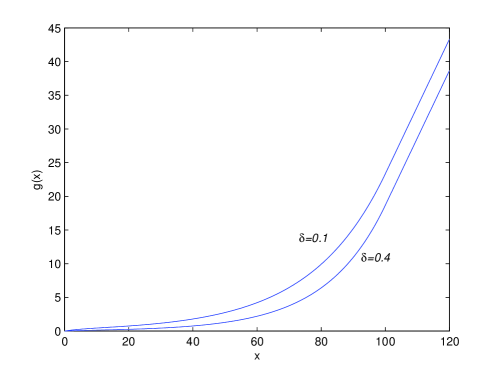
Figure 1. The optimal return function $g_{\delta}(x)$ as a function of $\delta$.   (Parameters: $\mu=2,\sigma=50,c=0.05,\alpha=0.5,\beta=8,T=300,b=100$ )

Example 5.2.

Let $\mu=2$, $\sigma^{2}=50$, $\delta=0.2$, $c=0.05$, $\alpha=0.5$, $\beta=8$, $T=300$. Let $b(\varepsilon)$ be the solution of $1-\phi(T,b)=\varepsilon$, where $\phi(T,b)$ is defined in Lemma 6.5. Thus given a constrained risk level $\varepsilon$ of bankrupt probability, $b(\varepsilon)$ is the associated dividends barrier. Figure 2 shows that the dividends barrier $b(\varepsilon)$ decreases with the constrained risk level $\varepsilon$.

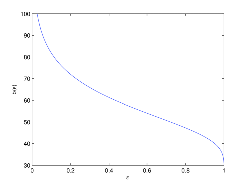
Figure 2. Dividends barrier $b(\varepsilon)$ as a function of $\varepsilon$.  (Parameters: $\mu=2,\sigma^{2}=50,\delta=0.2,c=0.05,\alpha=0.5,\beta=8,T=300$ )

Example 5.3.

Let $\mu=2$, $\delta=0.2$, $c=0.05$, $\alpha=0.5$, $\beta=8$, $T=300$. Let $b_{\sigma}(\varepsilon)$ be the solution of $1-\phi(T,b)=\varepsilon$, where $\phi(T,b)$ is defined in Lemma 6.5. We see from Figure 3 that at the same constrained risk level, the bigger the volatility rate $\sigma$ is, the higher the dividends barrier $b_{\sigma}(\varepsilon)$ is.

Figure 3. Dividends barrier $b_{\sigma}(\varepsilon)$ as a function of $\sigma^{2}$.  (Parameters: $\mu=2,\delta=0.2,c=0.05,\alpha=0.5,\beta=8,T=300$ )

Example 5.4.

Let $\mu=2$, $\sigma^{2}=50$ $\delta=0.2$, $c=0.05$, $\alpha=0.5$, $\beta=8$, $T=300$. Let $b_{\sigma}(\varepsilon)$ be the solution of $1-\phi(T,b)=\varepsilon$, where $\phi(T,b)$ is defined in Lemma 6.5. $R_{0}=x$ is the initial reserve and $\varepsilon$ is the constrained risk level of bankrupt probability. We see from figure 4 that the lower the initial reserve $x$ is, the higher the constrained risk level $\varepsilon$ is.

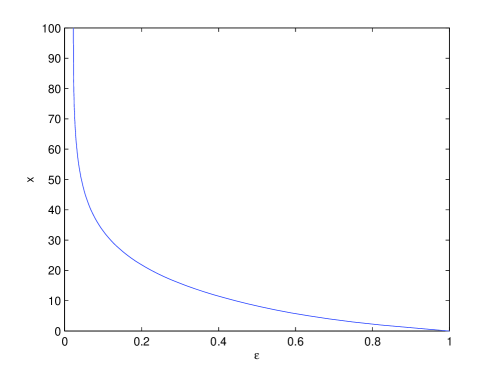
Figure 4. Initial reserve $x(\varepsilon)$ as a function of the risk restrained level $\varepsilon$.  (Parameters: $\mu=2,\sigma^{2}=50,\delta=0.2,c=0.05,\alpha=0.5,\beta=8,T=300$ )

Example 5.5.

Let $\sigma^{2}=50$, $\delta=0.2$, $c=0.05$, $\alpha=0.5$, $\beta=8$, $T=300$ and $b=100$. Figure 5 shows that the optimal return function $g_{\mu}(x)$ increases with the profit rate $\mu$.

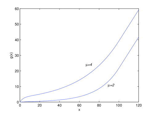
Figure 5. The optimal return function $g_{\mu}(x)$ as a function of $\mu$.   (Parameters: $\sigma^{2}=50,\delta=0.2,c=0.05,\alpha=0.5,\beta=8,T=300,b=100$ )

Example 5.6.

Let $\mu=2$, $\delta=0.2$, $c=0.05$, $\alpha=0.5$, $\beta=8$, $T=300$ and $b=100$. Figure 6 shows that the optimal return function $g_{\sigma}(x)$ increases with the volatility rate $\sigma^{2}$.

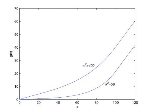
Figure 6. The optimal return function $g_{\sigma}(x)$ as a function of $\sigma^{2}$.   (Parameters: $\mu=2,\delta=0.2,c=0.05,\alpha=0.5,\beta=8,T=300,b=100$ )

Example 5.7.

Let $\mu=2$, $\sigma^{2}=50$, $\delta=0.2$, $c=0.05$, $\alpha=0.5$, $\beta=8$, $T=300$ and $b=100$. Set $x_{\alpha}=4.72$, $x_{\beta}=94.79$, the images of the optimal return function $g(x)$ as well as the optimal feedback control function $a^{*}(x)$ are as follows (see Figure 7 and Figure 8).

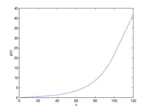
Figure 7. The optimal return function $g(x)$.   (Parameters: $\mu=2,\sigma^{2}=50,\delta=0.2,c=0.05,\alpha=0.5,\beta=8,T=300,b=100$ )

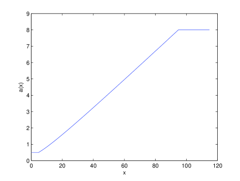
Figure 8. The optimal feedback control function $a(x)$.  (Parameters: $\mu=2,\sigma^{2}=50,\delta=0.2,c=0.05,\alpha=0.5,\beta=8,T=300,b=100$ )

6. Properties of $V(x,b)$ and Bankrupt Probability

In this section, we will discuss some important properties of the optimal return function $V(x,b)$ and bankrupt probability, which are used to prove the main result of this paper. The rigorous proofs of these properties will be given in the appendix. In view of Lemma 8.1 in the appendix, different value of $\frac{2\delta}{\mu}$ can lead to three different cases. When $\frac{2\delta}{\mu}<\alpha$, this case is the most complicated. We select this case as the basis of our discussion throughout the paper, and the results of the other two cases are almost same.

Lemma 6.1.

If $f(x)\in C^{2}$ and satisfies the following HJB equation and boundary conditions,

$$\left\{\begin{array}[]{l l l}\max\limits_{a\in[\alpha,\beta]}[\frac{1}{2}\sigma^{2}a^{2}f^{{}^{\prime\prime}}(x)+(\mu a-\delta)f^{{}^{\prime}}(x)-cf(x)]=0,\ \mbox{for}\ 0\leq x\leq b_{0},\\ f^{{}^{\prime}}(x)=1,\ \mbox{ for}\ x\geq b_{0},\\ f^{{}^{\prime\prime}}(x)=0,\ \mbox{ for}\ x\geq b_{0},\\ f(0)=0,\end{array}\right.$$ (6.5)

then we have

$$b_{0}=\inf\{x\geq 0:f^{\prime\prime}(x)=0\}$$

and

$$\left\{\begin{array}[]{l l l}\max\mathcal{L}f(x)\leq 0\ \mbox{and }\ f^{{}^{\prime}}(x)\geq 1\ \mbox{for}\ x\geq 0,\\ f(0)=0,\end{array}\right.$$

where $\mathcal{L}=\frac{1}{2}\sigma^{2}a^{2}\frac{d^{2}}{dx^{2}}+(\mu a-\delta)\frac{d}{dx}-c$.

Lemma 6.2.

Let $b>b_{0}$ be a predetermined variable. If $g\in C^{1}(R_{+})$, $g\in C^{2}(R_{+}\setminus\{b\})$ and satisfies the following HJB equation and boundary conditions,

$$\left\{\begin{array}[]{l l l}\max\limits_{a\in[\alpha,\beta]}[\frac{1}{2}\sigma^{2}a^{2}g^{{}^{\prime\prime}}(x)+(\mu a-\delta)g^{{}^{\prime}}(x)-cg(x)]=0,\ \mbox{for}\ 0\leq x\leq b,\\ g^{{}^{\prime}}(x)=1,\ \ \mbox{ for}\ \ x\geq b,\\ g^{{}^{\prime\prime}}(x)=0,\ \ \mbox{ for}\ \ x>b,\\ g(0)=0,\end{array}\right.$$ (6.11)

then we have

$$\left\{\begin{array}[]{l l l}\max\mathcal{L}g(x)\leq 0,\ \mbox{for}\ \ x\geq 0,\\ g^{{}^{\prime}}(x)\geq 1,\ \mbox{for}\ \ x\geq b,\\ g(0)=0,\end{array}\right.$$ (6.15)

where $b_{0}$ and $\mathcal{L}$ are the same as in Lemma 6.1, $g^{\prime\prime}(b):=g^{\prime\prime}(b-)$. The expression of $g(x)$ can be written as

$$g(x,b)=\left\{\begin{array}[]{l l l}k_{1}(e^{r_{+}(\alpha)}x-e^{r_{-}(\alpha)x}),\ 0\leq x<x_{\alpha},\\ k_{2}[\frac{\alpha\mu-2\delta}{2c}+\int_{x_{\alpha}}^{x}exp(-\frac{\mu}{\sigma^{2}}\int_{x_{\alpha}}^{y}\frac{dv}{a(v)})dy],\ x_{\alpha}\leq x<x_{\beta},\\ k_{3}e^{r_{+}(\beta)(x-b_{0})}+k_{4}e^{r_{-}(\beta)(x-b_{0})},\ x_{\beta}\leq x<b,\\ x-b+g_{3}(b),\ x\geq b,\end{array}\right.$$ (6.20)

where $r_{\pm}(x),x_{\alpha},x_{\beta},k_{1},k_{2},k_{3}$ and $k_{4}$ are given by (8.9), (8.10), (8.17), (8.21), (8.37) and (8.36), respectively.

Lemma 6.3.

Let $g(x,b)$ be as the same as in Lemma 6.2. Then $\frac{\partial}{\partial b}g(x,b)\leq 0$ holds for $b\geq b_{0}$.

Lemma 6.4.

The bankrupt probability $\mathbf{P}[\tau_{b}^{\pi^{*}_{b}}\leq T]$ is a strictly decreasing function w.r.t. the dividends barrier $b$ on $[x_{\beta},D)$, $D:=\inf\{b:\mathbf{P}[\tau_{b}^{\pi^{*}_{b}}\leq T]=0\}$, and $x_{\beta}$ is defined by (8.17).

From the proof of Lemma 6.2, for each $x\leq b$, if we define

$$a^{*}(x):=arg\ \max\limits_{a\in[\alpha,\beta]}[\frac{1}{2}\sigma^{2}a^{2}g^{{}^{\prime\prime}}(x)+(\mu a-\delta)g^{{}^{\prime}}(x)-cg(x)],$$ (6.21)

then it follows that $a^{*}(x)$ can be represented as

$$a^{*}(x)=\left\{\begin{array}[]{l l l}\alpha,\ \ 0\leq x<x_{\alpha},\\ a(x),\ \ x_{\alpha}\leq x<x_{\beta},\\ \beta,\ \ x\geq x_{\beta},\end{array}\right.$$ (6.25)

where $a(x)$ and $x_{\alpha},x_{\beta}$ are specified by (8.16), (8.10), (8.17), respectively. We now have the following lemma.

Lemma 6.5.

Let $a^{*}(x)$ be defined by (6.25), and define $\psi^{b}(T,x):={\bf{P}}[\tau^{\pi^{*}_{b}}_{x}\leq T]$, i.e., $\psi^{b}(T,x)$ is the bankrupt probability when the initial reserve of $\{R^{\pi^{*}_{b}}_{t}\}_{t\geq 0}$ is $x$ and dividends barrier is $b$. Let $\phi^{b}(t,y)\in C^{1}(0,\infty)\cap C^{2}(0,b)$ and satisfy the following partial differential equation and the boundary conditions,

$$\left\{\begin{array}[]{l l l}\phi_{t}^{b}(t,x)=\frac{1}{2}[a^{*}(x)]^{2}\sigma^{2}\phi_{xx}^{b}(t,x)+(a^{*}(x)\mu-\delta)\phi_{x}^{b}(t,x),\\ \phi^{b}(0,x)=1,\ \mbox{for}\ \ 0<x\leq b,\\ \phi^{b}(t,0)=0,\phi_{x}^{b}(t,b)=0,\ \mbox{for}\ t>0.\end{array}\right.$$ (6.29)

Then $\phi^{b}(T,x)=1-\psi^{b}(T,x)$, i.e., $\phi^{b}(T,x)$ is probability that the company will survive on $[0,T]$.

Lemma 6.6.

Let $\phi^{b}(t,x)$ solve the equation(6.29). Then $\phi^{b}(T,b)$ is continuous with respect to the dividends barrier $b$ on $[b_{0},+\infty)$.

7. Proof of Main Result

In this section, we prove the main result of this paper, which is described in Theorem 3.1. In order to do this, we first need the following.

Theorem 7.1.

Let $a^{*}_{b}(x)$ be defined by (6.25), and $f(x)$, $g(x,b)$ be as the same as in Lemma 6.1 and Lemma 6.2, respectively. Then
(i) If $b\leq b_{0}$, we have $V(x,b)=V(x,b_{0})=V(x)=f(x)$, the optimal policy associated with $V(x)$ is $\pi_{b_{o}}^{\ast}=\{a^{*}_{b_{0}}(R^{\pi_{b_{o}}^{\ast}}_{\cdot}),L^{\pi_{b_{o}}^{\ast}}_{\cdot}\}$, where the process $\{R^{\pi_{b_{o}}^{\ast}}_{t},L^{\pi_{b_{o}}^{\ast}}_{t}\}$ is uniquely determined by the following SDE,

$$\left\{\begin{array}[]{l l l}dR_{t}^{\pi_{b_{o}}^{\ast}}=(\mu a^{*}_{b_{0}}(R^{\pi_{b_{o}}^{\ast}}_{t})-\delta)dt+\sigma a^{*}_{b_{0}}(R^{\pi_{b_{o}}^{\ast}}_{t})d{W}_{t}-dL_{t}^{\pi_{b_{o}}^{\ast}},\\ R_{0}^{\pi_{b_{o}}^{\ast}}=x,\\ 0\leq R^{\pi_{b_{o}}^{\ast}}_{t}\leq b_{0},\\ \int^{\infty}_{0}I_{\{t:R^{\pi_{b_{o}}^{\ast}}_{t}<b_{0}\}}(t)dL_{t}^{\pi_{b_{o}}^{\ast}}=0.\end{array}\right.$$ (7.5)

(ii) If $b>b_{0}$, we have $V(x,b)=g(x,b)$ and the optimal policy $\pi_{b}^{\ast}$ is $\{a^{\ast}_{b}(R^{\pi_{b}^{\ast}}_{t}),L^{\pi_{b}^{\ast}}_{t}\}$, where $\{R^{\pi_{b}^{\ast}}_{t},L^{\pi_{b}^{\ast}}_{t}\}$ is uniquely determined by the following SDE

$$\left\{\begin{array}[]{l l l}dR_{t}^{\pi_{b}^{\ast}}=(\mu a^{*}_{b}(R^{\pi_{b}^{\ast}}_{t})-\delta)dt+\sigma a^{*}_{b}(R^{\pi_{b}^{\ast}}_{t})d{W}_{t}-dL_{t}^{\pi_{b}^{\ast}},\\ R_{0}^{\pi_{b}^{\ast}}=x,\\ 0\leq R^{\pi_{b}^{\ast}}_{t}\leq b,\\ \int^{\infty}_{0}I_{\{t:R^{\pi_{b}^{\ast}}_{t}<b\}}(t)dL_{t}^{\pi_{b}^{\ast}}=0.\end{array}\right.$$ (7.10)

Proof.

(i)  If $b\leq b_{0}$, since $\pi^{*}_{b_{0}}\in\Pi_{b_{0}}\subset\Pi_{b}$, we have $V(x,b_{0})\leq V(x,b)\leq V(x)$. It suffices to show $V(x)\leq f(x)=V(x,b_{0})$. Since its proof is similar to [7], we omit it here. (ii) If $b\geq b_{0}$, denote $g(x,b)$ by $g(x)$ for simplicity, for any admissible policy $\pi=\{a_{\pi},L^{\pi}\}$, we assume that $(R^{\pi}_{t},L^{\pi}_{t})$ is the process (2.3) associated with $\pi$. Let $\Lambda=\{s:L_{s-}^{\pi}\neq L_{s}^{\pi}\}$, $\hat{L}=\sum_{s\in\Lambda,s\leq t}(L_{s}^{\pi}-L_{s-}^{\pi})$ be the discontinuous part of $L_{s}^{\pi}$ and $\tilde{L}_{t}^{\pi}=L_{t}^{\pi}-\hat{L}_{t}^{\pi}$ be the continuous part of $L_{s}^{\pi}$. Applying generalized Itô formula to $e^{-c(t\wedge\tau^{\pi}_{x})}g(R_{t\wedge\tau^{\pi}_{x}}^{\pi})$, we have

$$e^{-c(t\wedge\tau^{\pi}_{x})}g(R_{t\wedge\tau^{\pi}_{x}}^{\pi}) = g(x)+\int_{0}^{t\wedge\tau^{\pi}_{x}}e^{-cs}\mathcal{L}g(R_{s}^{\pi})ds$$ (7.11)

$$+\int_{0}^{t\wedge\tau^{\pi}_{x}}a_{\pi}\sigma e^{-cs}g^{{}^{\prime}}(R_{s}^{\pi})d\mathcal{W}_{s}\mathcal{-}\int_{0}^{t\wedge\tau^{\pi}_{x}}e^{-cs}g^{{}^{\prime}}(R_{s}^{\pi})dL_{s}^{\pi}$$

$$+\sum\limits_{s\in\Lambda,s\leq t\wedge\tau^{\pi}_{x}}e^{-cs}[g(R_{s}^{\pi})-g(R_{s-}^{\pi})$$

$$-g^{{}^{\prime}}(R_{s-}^{\pi})(R_{s}^{\pi}-R_{s-}^{\pi})]$$

$$= g(x)+\int_{0}^{t\wedge\tau^{\pi}_{x}}e^{-cs}\mathcal{L}g(R_{s}^{\pi})ds$$

$$+\int_{0}^{t\wedge\tau^{\pi}_{x}}a_{\pi}\sigma e^{-cs}g^{{}^{\prime}}(R_{s}^{\pi})d\mathcal{W}_{s}\mathcal{-}\int_{0}^{t\wedge\tau^{\pi}_{x}}e^{-cs}g^{{}^{\prime}}(R_{s}^{\pi})d\tilde{L}_{s}^{\pi}$$

$$+\sum\limits_{s\in\Lambda,s\leq t\wedge\tau^{\pi}_{x}}e^{-cs}[g(R_{s}^{\pi})-g(R_{s-}^{\pi}))],$$

where

$$\mathcal{L}=\frac{1}{2}a^{2}\sigma^{2}\frac{d^{2}}{dx^{2}}+(\mu a-\delta)\frac{d}{dx}-c.$$

In view of the HJB equation (6.11), $\mathcal{L}g(R_{s}^{\pi})$ is always non-positive, so is the second term on the right hand side of(7.11). By taking mathematical expectations at both sides of (7.11), we get

$${\bf E}\big{[}e^{-c(t\wedge\tau^{\pi}_{x})}g(R_{t\wedge\tau^{\pi}_{x}}^{\pi})\big{]} \leq g(x)-{\bf E}\big{[}\int_{0}^{t\wedge\tau^{\pi}_{x}}e^{-cs}g^{{}^{\prime}}(R_{s}^{\pi})d\tilde{L}_{s}^{\pi}\big{]}$$

$$+{\bf E}\big{[}\sum\limits_{s\in\Lambda,s\leq t\wedge\tau^{\pi}_{x}}e^{-cs}[g(R_{s}^{\pi})-g(R_{s-}^{\pi})]\big{]}.$$

Since $g^{{}^{\prime}}(x)\geq 1$, for $x\geq b$,

$$g(R_{s}^{\pi})-g(R_{s-}^{\pi})\leq-(L_{s}^{\pi}-L_{s-}^{\pi}),$$ (7.13)

which, together with (7), implies that

$${\bf E}\big{[}e^{-c(t\wedge\tau^{\pi}_{x})}g(R_{t\wedge\tau^{\pi}_{x}}^{\pi})\big{]} + {\bf E}\big{[}\int_{0}^{t\wedge\tau^{\pi}_{x}}e^{-cs}dL_{s}^{\pi}\big{]}\leq g(x).$$ (7.14)

By the definition of $\tau^{\pi}_{x}$ and $g(0)=0$, letting $t\rightarrow\infty$ in (7.14), we get

$$\liminf\limits_{t\rightarrow\infty}e^{-c(t\wedge\tau^{\pi}_{x})}g(R_{t\wedge\tau^{\pi}_{x}}^{\pi}) = e^{-c\tau}g(0)I_{\{\tau^{\pi}_{x}<\infty\}}$$ (7.15)

$$+\liminf\limits_{t\rightarrow\infty}e^{-ct}g(R_{t})I_{\{\tau^{\pi}_{x}=\infty\}}$$

$$\geq 0.$$

We deduce from (7.14) and (7.15) that

$$J(x,\pi)={\bf E}\big{[}\int_{0}^{\tau^{\pi}_{x}}e^{-cs}dL_{s}^{\pi}\big{]}\leq g(x).$$

So

$$V(x,b)\leq g(x).$$ (7.16)

If we choose the control policy $\pi_{b}^{\ast}=\{a^{*}_{b}(R^{\pi_{b}^{\ast}}_{\cdot}),L^{\pi_{b}^{\ast}}_{\cdot}\}$, which is uniquely determined by SDE (7.10), then all the inequalities above become equalities. Hence

$$V(x,b)=g(x).$$

So we have

$$V(x,b)=g(x,b).$$ (7.17)

∎

Now we prove the main result of this paper. Proof of Theorem 3.1. If $\mathbf{P}[\tau_{b_{0}}^{\pi^{*}_{b_{0}}}\leq T]\leq\varepsilon$, the bankrupt probability constraint does not work and it turns to a usual optimal control problem, thus the conclusion is obvious. If $\mathbf{P}[\tau_{b_{0}}^{\pi^{*}_{b_{0}}}\leq T]>\varepsilon$, then by lemmas 6.4-6.6 there exists a unique $b^{\ast}$ solving the equation $\mathbf{P}\{\tau_{b}^{\pi^{*}_{b}}\leq T\}=\varepsilon$. Moreover, $b^{\ast}=\inf\{b:b\in\mathfrak{B}\}>b_{0}$. By Theorem 7.1 and Lemma 6.3, $V(x,b)=g(x,b)$ for $b>b_{0}$ and $V(x,b)$ is decreasing w.r.t. $b$. Therefore, we know that $b^{\ast}$ meets (3.6) and (3.7). So the optimal policy associated with the optimal return function $V(x,b^{*})$ is $\{a^{\ast}_{b^{*}}(R^{\pi_{b^{*}}^{\ast}}_{t}),L^{\pi_{b^{*}}^{\ast}}_{t}\}$, which is uniquely determined by SDE (3.12). Due to the fact $b^{*}>b_{0}$, the inequity (3.13) is a direct consequence of Lemma 6.3. Thus we complete the proof.   $\Box$

8. Appendix

In this section, we first discuss some useful arguments, then we give the proofs of the lemmas used in the previous sections. Due to the mathematical model presented by (2.2), $a(t)$ is required to take values in the interval $\alpha,\beta$, where $0<\alpha<\beta<+\infty$. Thus, $a(t)\mu-\delta$ may be negative because $\delta>0$. If $\beta\mu\leq\delta$, there exists a trivial solution to the corresponding HJB equations, which has been proved by Choulli, Taksar, and Zhou[7]. In the next section, we always assume that $\beta\mu\geq\delta$. Then the following statements are valid.

Lemma 8.1.

Let $\beta\mu>0$. Then
(i) $\frac{2\delta}{\mu}<\alpha$ if and only if $a(0)<\alpha$. In this case,

$$a(0)=\frac{\mu\alpha^{2}}{2(\mu\alpha-\delta)}.$$ (8.1)

(ii) $\alpha\leq\frac{2\delta}{\mu}<\beta$ if and only if $\alpha\leq a(0)<\beta$. In this case,

$$a(0)=\frac{2\delta}{\mu}.$$ (8.2)

(iii) $\beta\leq\frac{2\delta}{\mu}$ if and only if $a(0)\geq\beta$. In this case,

$$a(0)=\frac{\mu\beta^{2}}{2(\mu\beta-\delta)}.$$ (8.3)

Proof.

See Choulli, Taksar and Zhou[7] for details. ∎

Due to Lemma 8.1, there are three different cases to investigate. Since the proof of each case is similar, we only give sketch proofs of lemmas in case (i). Thus we suppose $\frac{2\delta}{\mu}<\alpha$ throughout the following procedure to prove these lemmas. Proof of lemma 6.1.  The complete proof is given in Choulli, Taksar and Zhou[7](2003).   $\Box$

Proof of lemma 6.2. Step 1. For each $x\geq 0$ and $a\geq 0$, define

$$h(x,a)=\frac{1}{2}\sigma^{2}a^{2}g^{{}^{\prime\prime}}(x)+(\mu a-\delta)g^{{}^{\prime}}(x)-cg(x).$$ (8.4)

Then, by differentiating $h(x,a)$ w.r.t. $a$, we get the maximizing function of $h(x,a)$

$$a(x)=-\frac{\mu g^{{}^{\prime}}(x)}{\sigma^{2}g^{{}^{\prime\prime}}(x)},\ \ x\geq 0.$$ (8.5)

In view of Lemma 8.1 (i), $a(x)\leq\alpha$ for all $x$ in the right neighborhood of 0. Substituting $a=\alpha$ into (6.11), and solving the resulting second-order linear ODE, we get

$$g(x)=k_{1}(e^{r_{+}(\alpha)}x-e^{r_{-}(\alpha)x}),\ \ 0\leq x<x_{\alpha},$$ (8.6)

where $k_{1}$ and $x_{\alpha}$ are to be determined and for $x>0$

$$\left\{\begin{array}[]{l l l}r_{+}(x)=\frac{-(\mu x-\delta)+\sqrt{(\mu x-\delta)^{2}+2\sigma^{2}cx^{2}}}{\sigma^{2}x^{2}}\\ r_{-}(x)=\frac{-(\mu x-\delta)-\sqrt{(\mu x-\delta)^{2}+2\sigma^{2}cx^{2}}}{\sigma^{2}x^{2}}.\end{array}\right.$$ (8.9)

Due to (8.5) and (8.6), for $x>0$

$$a^{{}^{\prime}}(x)=\frac{-\mu r_{+}(\alpha)r_{-}(\alpha)(r_{+}(\alpha)-r_{-}(\alpha))^{2}e^{(r_{+}(\alpha)+r_{-}(\alpha))x}}{\sigma^{2}(g^{{}^{\prime\prime}}(x))^{2}}>0.$$

Therefore $a(x)$ increases to $\alpha$ at the point $x_{\alpha}$ given by

$$x_{\alpha}=\frac{1}{r_{+}(\alpha)-r_{-}(\alpha)}log(\frac{r_{-}(\alpha)(\mu+\alpha\sigma^{2}r_{-}(\alpha))}{r_{+}(\alpha)(\mu+\alpha\sigma^{2}r_{+}(\alpha))})>0.$$ (8.10)

Step 2. In view of Proposition 8 in [7], $\alpha\leq a(x)\leq\beta$ in the right neighborhood of $x_{\alpha}$. From (8.5), we get

$$g^{{}^{\prime\prime}}(x)=-\frac{\mu g^{{}^{\prime}}(x)}{\sigma^{2}a(x)}.$$ (8.11)

Substituting (8.11) into (6.11), differentiating the resulting equation, and using (8.11) again, we obtain

$$a^{{}^{\prime}}(x)=\frac{\mu^{2}+2c\sigma^{2}}{\mu\sigma^{2}}(1-\frac{u}{a(x)}),$$ (8.12)

with

$$u\equiv\frac{2\delta\mu}{\mu^{2}+2c^{2}\sigma^{2}}.$$ (8.13)

Integrating (8.12), we get

$$G(a(x))=\frac{\mu^{2}+2c\sigma^{2}}{\mu\sigma^{2}}(x-x_{\alpha})+G(\alpha),$$ (8.14)

where

$$G(z)=z+ulog(z-u).$$ (8.15)

Therefore

$$a(x)=G^{-1}(\frac{\mu^{2}+2c\sigma^{2}}{\mu\sigma^{2}}(x-x_{\alpha})+G(\alpha)).$$ (8.16)

Obviously, $a(x)$ is increasing. Let $a(x_{\beta})=\beta$, we get

$$x_{\beta} = \frac{\mu\sigma^{2}}{\mu^{2}+2c\sigma^{2}}[G(\beta)-G(\alpha)]+x_{\alpha}$$ (8.17)

$$= \frac{\mu\sigma^{2}}{\mu^{2}+2c\sigma^{2}}(\beta-\alpha)+\frac{\mu\sigma^{2}u}{\mu^{2}+2c\sigma^{2}}log(\frac{\beta-u}{\alpha-u})+x_{\alpha}.$$

Solving (8.11),(8.15) and (8.16), we obtain

$$g(x)=g(x_{\alpha})+g^{{}^{\prime}}(x_{\alpha})\int_{x_{\alpha}}^{x}exp(-\frac{\mu}{\sigma^{2}}\int_{x_{\alpha}}^{y}\frac{dv}{a(v)})dy,\ \ x_{\alpha}\leq x<x_{\beta},$$

where $g(x_{\alpha})$ and $g^{{}^{\prime}}(x_{\alpha})$ are free constants to be determined. From (8.6) and (8.10), we deduce

$$g(x_{\alpha})=\frac{\alpha\mu-2\delta}{2c}g^{{}^{\prime}}(x_{\alpha})$$ (8.19)

Let

$$k_{2}\equiv g^{{}^{\prime}}(x_{\alpha}),$$ (8.20)

Then (8.6) and (8.19) imply

$$k_{1}=\frac{\alpha\mu-2\delta}{2c(e^{r_{+}(\alpha)x_{\alpha}}-e^{r_{-}(\alpha)x_{\alpha}})}k_{2}$$ (8.21)

Substituting (8.19) and (8.20) into (8), we get

$$g(x)=k_{2}[\frac{\alpha\mu-2\delta}{2c}+\int_{x_{\alpha}}^{x}exp(-\frac{\mu}{\sigma^{2}}\int_{x_{\alpha}}^{y}\frac{dv}{a(v)})dy],\ x_{\alpha}\leq x<x_{\beta}.$$ (8.22)

Step 3. In view of Proposition 9 in [7], $a(x)\geq\beta$ holds for $x\geq x_{\beta}$. Substituting $a=\beta$ into (6.11), and solving it, we get the following solution

$$g(x)=k_{3}e^{r_{+}(\beta)(x-b_{0})}+k_{4}e^{r_{-}(\beta)(x-b_{0})},\ x_{\beta}\leq x<b,$$ (8.23)

where $k_{3},k_{4}$ are free constants to be determined and $r_{\pm}(\beta)$ are given by (8.9). For $x\geq b$, the solution has the following form

$$g(x)=x-b+k_{3}e^{r_{+}(\beta)(b-b_{0})}+k_{4}e^{r_{-}(\beta)(b-b_{0})},\ x\geq b.$$ (8.24)

Next we apply the principle of smooth fit to determine the unknown constants above. Note that

$$\left\{\begin{array}[]{l l l}g(x_{\beta}-)=g(x_{\beta}+)\\ g^{{}^{\prime}}(x_{\beta}-)=g^{{}^{\prime}}(x_{\beta}+),\end{array}\right.$$ (8.27)

we arrive at

$$\left\{\begin{array}[]{l l l}k_{2}\xi=k_{3}e^{r_{+}(\beta)(x_{\beta}-b_{0})}+k_{4}e^{r_{-}(\beta)(x_{\beta}-b_{0})}\\ k_{2}\eta=k_{3}r_{+}(\beta)e^{r_{+}(\beta)(x_{\beta}-b_{0})}+k_{4}r_{-}(\beta)e^{r_{-}(\beta)(x_{\beta}-b_{0})},\end{array}\right.$$ (8.30)

where

$$\left\{\begin{array}[]{l l l}\xi=\frac{\alpha\mu-2\delta}{2c}+\int_{x_{\alpha}}^{x_{\beta}}exp(-\frac{\mu}{\sigma^{2}}\int_{x_{\alpha}}^{y}\frac{dv}{a(v)})dy\\ \eta=exp(-\frac{\mu}{\sigma^{2}}\int_{x_{\alpha}}^{x_{\beta}}\frac{dv}{a(v)}).\end{array}\right.$$ (8.33)

Solving (8.30) for $k_{3}$ and $k_{4}$, we get

$$\left\{\begin{array}[]{l l l}k_{3}=\frac{\eta-\xi r_{-}(\beta)}{(r_{+}(\beta)-r_{-}(\beta))e^{r_{+}(\beta)(x_{\beta}-b_{0})}}k_{2}\equiv Ak_{2}\\ k_{4}=\frac{\xi r_{+}(\beta)-\eta}{(r_{+}(\beta)-r_{-}(\beta))e^{r_{-}(\beta)(x_{\beta}-b_{0})}}k_{2}\equiv Bk_{2}.\end{array}\right.$$ (8.36)

Substituting (8.36) into (8.23) and using $g^{{}^{\prime}}(b-)=1$, we obtain

$$k_{2}=\frac{1}{Ar_{+}(\beta)e^{r_{+}(\beta)(b-b_{0})}+Br_{-}(\beta)e^{r_{-}(\beta)(b-b_{0})}}.$$ (8.37)

Thus, $k_{1},k_{2},k_{3},k_{4}$ are determined by (8.21),(8.36) and (8.37). We claim that

$$g^{{}^{\prime\prime}}(b_{-})\geq 0.$$ (8.38)

In order to prove this statement, we consider $f(x)$ in Lemma 6.1 and notice that $A$ and $B$ in (8.36) have the same expression both in $f(x)$ and $g(x)$. Since $f^{{}^{\prime}}(b_{0})=1$ and $f^{{}^{\prime\prime}}(b_{0})=0$,

$$\left\{\begin{array}[]{l l l}k^{f}_{2}(Ar_{+}(\beta)+Br_{-}(\beta))=1\\ k^{f}_{2}(Ar^{2}_{+}(\beta)+Br^{2}_{-}(\beta))=0,\end{array}\right.$$ (8.41)

where $k^{f}_{2}$ is the corresponding constant in Lemma 6.1. From (8.41), we know that $A<0,B>0$ due to $r_{+}(\beta)>0,r_{-}(\beta)<0)$ and $k^{f}_{2}>0$ in $f(x)$. In addition, if we let

$$l(b)\equiv g^{{}^{\prime\prime}}_{3}(b-)=\frac{Ar^{2}_{+}(\beta)e^{r_{+}(\beta)(b-b_{0})}+Br^{2}_{-}(\beta)e^{r_{-}(\beta)(b-b_{0})}}{Ar_{+}(\beta)e^{r_{+}(\beta)(b-b_{0})}+Br_{-}(\beta)e^{r_{-}(\beta)(b-b_{0})}},$$ (8.42)

then,

$$\frac{\partial l}{\partial b} = \frac{AB(r^{3}_{+}(\beta)r_{-}(\beta)+r_{+}(\beta)r^{3}_{-}(\beta)-2r^{2}_{+}(\beta)r^{2}_{-}(\beta))e^{(r_{+}(\beta)+r_{(}\beta))(b-b_{0})}}{(Ar_{+}(\beta)e^{r_{+}(\beta)(b-b_{0})}+Br_{-}(\beta)e^{r_{-}(\beta)(b-b_{0})})^{2}}$$

$$> 0$$

holds for $A>0,B<0,r_{+}(\beta)>0$ and $r_{-}(\beta)<0$. Since $b>b_{0}$, we conclude that

$$g^{{}^{\prime\prime}}(b-)=l(b)>l(b_{0})=\tilde{g}^{{}^{\prime\prime}}(b_{0})=0,$$ (8.44)

where $\tilde{g}(x)$ is the solution of (6.11) with replacing $b$ by $b_{0}$. Step 4. Now we only need to prove the solution $g(x)$ satisfies (6.11). It suffices to prove the following conditions,

$$\max\limits_{a\in[\alpha,\beta]}[\frac{1}{2}\sigma^{2}a^{2}g^{{}^{\prime\prime}}(x)+(\mu a-\delta)g^{{}^{\prime}}(x)-cg(x)]=0,\ \mbox{for}\ x\geq b.$$

By (6.11), (8.44) and noticing that $g^{{}^{\prime}}(b-)=1$, we get

$$\max\mathcal{L}g(x) = \mu a-\delta-c(x-b+g(b))$$ (8.45)

$$\leq \mu a-\delta-cg(b)$$

$$\leq \frac{1}{2}\sigma^{2}a^{2}g^{{}^{\prime\prime}}(b-)+(\mu a-\delta)g^{{}^{\prime}}_{3}(b-)-cg(b)$$

$$\leq 0.$$

Thus, we complete the proof. We summarize the solution as follows. For $\frac{2\delta}{\mu}<\alpha$,

$$g(x)=\left\{\begin{array}[]{l l l}k_{1}(e^{r_{+}(\alpha)x}-e^{r_{-}(\alpha)x}),\ \ 0\leq x<x_{\alpha},\\ k_{2}[\frac{\alpha\mu-2\delta}{2c}+\int_{x_{\alpha}}^{x}\exp(-\frac{\mu}{\sigma^{2}}\int_{x_{\alpha}}^{y}\frac{dv}{a(v)})dy],\ \ x_{\alpha}\leq x<x_{\beta},\\ k_{3}e^{r_{+}(\beta)(x-b_{0})}+k_{4}e^{r_{-}(\beta)(x-b_{0})},\ \ x_{\beta}\leq x<b,\\ x-b+k_{3}e^{r_{+}(\beta)(b-b_{0})}+k_{4}e^{r_{-}(\beta)(b-b_{0})},\ \ x\geq b,\end{array}\right.$$ (8.50)

where $r_{\pm}(x),x_{\alpha},x_{\beta},k_{1},k_{2},k_{3}$ and $k_{4}$ are defined by (8.9), (8.10), (8.17), (8.21), (8.37) and (8.36), respectively.   $\Box$ Proof of lemma 6.3.  For $b\geq b_{0},A<0,B>0$, together with (8.42) and (8), we have

$$\frac{\partial}{\partial b}g(b,x) = -\frac{(\alpha\mu-2\delta)}{2c(e^{r_{+}(\alpha)x_{\alpha}-r_{-}(\alpha)x_{\alpha}})}$$

$$\times\frac{Ar^{2}_{+}(\beta)e^{r_{+}(\beta)(b-b_{0})}+Br^{2}_{-}(\beta)e^{r_{-}(\beta)(b-b_{0})}}{(Ar_{+}(\beta)e^{r_{+}(\beta)(b-b_{0})}+Br_{-}(\beta)e^{r_{-}(\beta)(b-b_{0})})^{2}}$$

$$\leq 0,\ \ \ 0\leq x<x_{\alpha};$$

$$\frac{\partial}{\partial b}g(b,x) = -(\frac{\alpha\mu-2\delta}{2c}+\int_{x_{\alpha}}^{x}exp(-\frac{\mu}{\sigma^{2}}\int_{x_{\alpha}}^{y}\frac{dv}{a(v)})dy)$$

$$\times\frac{Ar^{2}_{+}(\beta)e^{r_{+}(\beta)(b-b_{0})}+Br^{2}_{-}(\beta)e^{r_{-}(\beta)(b-b_{0})}}{(Ar_{+}(\beta)e^{r_{+}(\beta)(b-b_{0})}+Br_{-}(\beta)e^{r_{-}(\beta)(b-b_{0})})^{2}}$$

$$\leq 0,\ \ \ x_{\alpha}\leq x<x_{\beta};$$

$$\frac{\partial}{\partial b}g(b,x) = (Ae^{r_{+}(\beta)(b-b_{0})}+Be^{r_{-}(\beta)(b-b_{0})})$$

$$\times\frac{(Ar^{2}_{+}(\beta)e^{r_{+}(\beta)(b-b_{0})}+Br^{2}_{-}(\beta)e^{r_{-}(\beta)(b-b_{0})})}{(Ar_{+}(\beta)e^{r_{+}(\beta)(b-b_{0})}+Br_{-}(\beta)e^{r_{-}(\beta)(b-b_{0})})^{2}}$$

$$\leq 0,\ \ \ x_{\beta}\leq x<b;$$

$$\frac{\partial}{\partial b}g(b,x) = (Ae^{r_{+}(\beta)(b-b_{0})}+Be^{r_{-}(\beta)(b-b_{0})})$$

$$\times\frac{(Ar^{2}_{+}(\beta)e^{r_{+}(\beta)(b-b_{0})}+Br^{2}_{-}(\beta)e^{r_{-}(\beta)(b-b_{0})})}{(Ar_{+}(\beta)e^{r_{+}(\beta)(b-b_{0})}+Br_{-}(\beta)e^{r_{-}(\beta)(b-b_{0})})^{2}}$$

$$\leq 0,\ \ \ x\geq b.$$

Thus, the proof is completed.  $\Box$ Proof of lemma 6.4. We can prove that $\mathbf{P}[\tau_{b}^{\pi^{*}_{b}}\leq T]$ is decreasing in $b$ along the lines of Theorem 3.1 in [17](2008). Here we only need to prove that $\mathbf{P}[\tau_{b}^{\pi^{*}_{b}}\leq T]$ is strictly decreasing in $b$ on $[x_{\beta},D)$. We denote $\mathbf{P}[\tau_{b}^{\pi^{*}_{b}}\leq T]$ by $\mathbf{P}[\tau_{b}^{b}\leq T]$ for simplicity. For any $b_{1},b_{2}$ satisfying $D\geq b_{2}\geq b_{1}\geq x_{\beta}$, we need to prove that

$$\mathbf{P}[\tau_{b_{1}}^{b_{1}}\leq T]-\mathbf{P}[\tau_{b_{2}}^{b_{2}}\leq T]>0$$

By comparison theorem, we have

$$\mathbf{P}[\tau_{b_{1}}^{b_{1}}\leq T]-\mathbf{P}[\tau_{b_{2}}^{b_{2}}\leq T]\geq\mathbf{P}[\tau_{b_{1}}^{b_{2}}\leq T]-\mathbf{P}[\tau_{b_{2}}^{b_{2}}\leq T].$$

So we the proof can be reduced to proving that

$$\mathbf{P}[\tau_{b_{1}}^{b_{2}}\leq T]-\mathbf{P}[\tau_{b_{2}}^{b_{2}}\leq T]>0.$$ (8.52)

Define stochastic processes $R_{t}^{(1)}$, $R_{t}^{(2)}$, $R_{t}^{(3)}$, $R_{t}^{(4)}$ by the following SDEs:

$$dR_{t}^{(1)} = [\mu a_{b_{2}}^{*}(R_{t}^{(1)})-\delta]dt+a_{b_{2}}^{*}(R_{t}^{(1)})\sigma d\mathcal{W}_{t}-dL_{t}^{b_{2}},R_{0}^{(1)}=b_{1};$$

$$dR_{t}^{(2)} = [\mu a_{b_{2}}^{*}(R_{t}^{(2)})-\delta]dt+a_{b_{2}}^{*}(R_{t}^{(2)})\sigma d\mathcal{W}_{t}-dL_{t}^{b_{2}},R_{0}^{(2)}=b_{2};$$

$$dR_{t}^{(3)} = [\mu a_{b_{2}}^{*}(R_{t}^{(3)})-\delta]dt+a_{b_{2}}^{*}(R_{t}^{(3)})\sigma d\mathcal{W}_{t}-dL_{t}^{b_{2}},R_{0}^{(3)}=\frac{b_{1}+b_{2}}{2};$$

$$dR_{t}^{(4)} = [\mu a_{b_{2}}^{*}(R_{t}^{[4]})-\delta]dt+a_{b_{2}}^{*}(R_{t}^{(4)})\sigma d\mathcal{W}_{t},R_{0}^{(4)}=\frac{b_{1}+b_{2}}{2},$$

respectively, where $D\geq b_{2}\geq b_{1}\geq x_{\beta}$ and $a^{*}(\cdot)$ is defined by (6.25). First, let $\tau^{b_{1}}=\inf\limits_{t\geq 0}\{t:R_{t}^{(2)}=b_{1}\}$, $A=\{\tau^{b_{1}}\leq T\}$, $B=\big{\{}\sl R_{t}^{(2)}$ will go to bankruptcy in a time interval $[\tau^{b_{1}},\tau^{b_{1}}+T]$ and $\tau^{b_{1}}\leq T\big{\}}$, $D=\{\inf\limits_{0\leq t\leq T}R_{t}^{(3)}>b_{1}\}$ and $E=\{\inf\limits_{0\leq t\leq T}R_{t}^{(4)}>b_{1},\sup\limits_{0\leq t\leq T}R_{t}^{(4)}<b_{2}\}$. Then

$$\{\tau_{b_{2}}^{b_{2}}\leq T\}\subset B\subset A.$$ (8.53)

Moreover, by using strong Markov property of $R_{t}^{[2]}$, we have

$$\mathbf{P}[\tau_{b_{1}}^{b_{2}}\leq T]=\mathbf{P}[B|A].$$ (8.54)

By comparison theorem on SDE, we have

$$\mathbf{P}(A^{c})\geq\mathbf{P}(D)\geq\mathbf{P}(E).$$ (8.55)

Since $a_{b_{2}}^{*}(x)=\beta$ we have

$$R_{t}^{(4)}=\frac{b_{1}+b_{2}}{2}+[\mu\beta-\delta]t+\sigma\mathcal{W}_{t}\ \mbox{ on $E$}.$$ (8.56)

We deduce from (8.56) and properties of Brownian motion with drift (cf. Andrei,Borodin,Paavo,Salminen [1] (2002)) that

$$\mathbf{P}(E)=\frac{e^{-\mu^{\prime 2}T/2}}{\sqrt{2\pi T}}\sum_{k=-\infty}^{\infty}\int_{b_{1}/\sigma\beta}^{b_{2}/\sigma\beta}e^{\mu^{\prime}(z-x)}[(e^{-(z-x+\frac{2k(b_{2}-b_{1})}{\sigma\beta})^{2}/2T})$$

$$-(e^{-(z+x-\frac{2b_{1}-2k(b_{2}-b_{1})}{\sigma\beta})^{2}/2T})]dz>0,$$

where $\mu^{\prime}=(\beta\mu-\delta)/\sigma$ and $x=\frac{b_{1}+b_{2}}{2\sigma\beta}$. Thus we get

$$\mathbf{P}(A^{c})>0.$$ (8.57)

We also know from Theorem 4.1 that $\mathbf{P}[\tau_{b_{1}}^{b_{2}}\leq T]\geq\mathbf{P}[\tau_{b_{2}}^{b_{2}}\leq T]>0$, which together with (8.53), (8.54) and (8.57), implies that

$$\mathbf{P}[\tau_{b_{1}}^{b_{2}}\leq T]-\mathbf{P}[\tau_{b_{2}}^{b_{2}}\leq T] \geq \mathbf{P}[\tau_{b_{1}}^{b_{2}}\leq T]-\mathbf{P}(B)$$

$$= \mathbf{P}[\tau_{b_{1}}^{b_{2}}\leq T]-\mathbf{P}(A)\mathbf{P}(B|A)$$

$$= \mathbf{P}[\tau_{b_{1}}^{b_{2}}\leq T](1-\mathbf{P}(A))$$

$$= \mathbf{P}[\tau_{b_{1}}^{b_{2}}\leq T]\mathbf{P}(A^{c})$$

$$> 0.$$

Thus the proof is completed. $\Box$

Proof of lemma 6.5.   Let $\phi(t,x)\equiv\phi^{b}(t,x)$. Setting $\tau_{x}^{b}:=\tau_{x}^{\pi^{*}_{b}}$ and applying the generalized Itô formula to $(R^{\pi_{b}^{\ast},x}_{t},L_{t}^{\pi_{b}^{\ast}})$ and $\phi(t,x)$ we have for $0<x\leq b$,

$$\phi(T-(t\wedge\tau_{x}^{b}),R^{\pi_{b}^{\ast},x}_{t\wedge\tau_{x}^{b}}) = \phi(T,x)$$

$$+ \int_{0}^{t\wedge\tau_{x}^{b}}(\frac{1}{2}a^{*2}(R^{\pi_{b}^{\ast},x}_{s})\sigma^{2}\phi_{yy}(T-s,R^{\pi_{b}^{\ast},x}_{s})$$

$$+ (a^{*}_{b}(R^{\pi_{b}^{\ast},x}_{s})\mu-\delta)\phi_{x}(T-s,R^{\pi_{b}^{\ast},x}_{s})$$

$$- \phi_{t}(T-s,R^{\pi_{b}^{\ast},x}_{s}))ds-\int_{0}^{t\wedge\tau_{x}^{b}}\phi_{y}(T-s,R^{\pi_{b}^{\ast},x}_{s})dL_{s}^{b}$$

$$+ \int_{0}^{t\wedge\tau_{x}^{b}}a^{*}(R^{\pi_{b}^{\ast},x}_{s})\sigma\phi_{x}(T-s,R^{\pi_{b}^{\ast},x}_{s})dW_{s}.$$

Setting $t=T$ and taking mathematical expectation at both sides of (8) yield that

$$\phi(T,x) = \mathbf{E}[\phi(T-(T\wedge\tau_{x}^{b}),R^{\pi_{b}^{\ast},x}_{T\wedge\tau_{x}^{b}})]$$

$$= \mathbf{E}[\phi(0,R^{\pi_{b}^{\ast},x}_{T})1_{T<\tau_{x}^{b}}]+\mathbf{E}[\phi(T-\tau_{x}^{b},0)1_{T\geq\tau_{x}^{b}})]$$

$$= \mathbf{E}[1_{T<\tau_{x}^{b}}]$$

$$= 1-\psi(T,x).$$

Thus we complete the proof.  $\Box$

Define $u(x):=\frac{1}{2}a^{*2}(x)\sigma^{2}$, $v(x):=a^{*2}(x)\mu-\delta$, the equation (4.13) becomes

$$\phi_{t}^{b}(t,x)=u(x)\phi_{xx}^{b}(t,x)+v(x)\phi_{x}^{b}(t,x).$$ (8.59)

Obviously, $u(x)$ and $v(x)$ are continuous in $[0,b]$ due to the fact that $a^{*}(x)$ is continuous w.r.t $x$. Thus there exists a unique solution in $C^{1}(0,\infty)\cap C^{2}(0,b)$ for (6.29). Moreover, $u^{{}^{\prime}}(x)$, $v^{{}^{\prime}}(x)$, $u^{{}^{\prime\prime}}(x)$ are bounded in $(0,x_{\alpha})$, $(x_{\alpha},x_{\beta})$, $(x_{\beta},b)$, respectively. Now we are ready to prove that the bankrupt probability $\psi^{b}(T,b)$ is continuous with respect to the dividends barrier $b(b\geq b_{0})$. Proof of lemma 6.6.  It suffices to prove that $\phi^{b}(t,x)$ is continuous in b. Let $x=by$ and $\theta^{b}(t,y)=\phi^{b}(t,by)$, the equation (6.29) becomes

$$\left\{\begin{array}[]{l l l}\theta_{t}^{b}(t,y)=[u(by)/b^{2}]\theta_{yy}^{b}(t,z)+[v(by)/b]\theta_{y}^{b}(t,y),\\ \theta^{b}(0,y)=1,\ \mbox{for}\ 0<y\leq 1,\\ \theta^{b}(t,0)=0,\theta_{y}^{b}(t,1)=0,\ \mbox{for}\ t>0.\end{array}\right.$$ (8.63)

So the proof of Lemma 6.6 can be reduced to proving $\lim\limits_{b_{2}\rightarrow b_{1}}\theta^{b_{2}}(t,1)=\theta^{b_{1}}(t,1)$ for fixed $b_{1}>b_{0}$. Setting $w(t,y)=\theta^{b_{2}}(t,y)-\theta^{b_{1}}(t,y)$ and noticing that $\theta^{b}(t,y)$ is continuous at $y=1$ for any $b\geq b_{0}$, it suffices to show that

$$\int_{0}^{t}\int_{0}^{1}w^{2}(s,y)dyds\rightarrow 0,\ \mbox{as}\ b_{2}\rightarrow b_{1}.$$ (8.64)

Thus we have

$$\left\{\begin{array}[]{l l l}w_{t}(t,y)&=&[u(b_{2}y)/b_{2}^{2}]w_{yy}(t,y)+[v(b_{2}y)/b_{2}]w_{y}(t,y)\\ &+&\{u(b_{2}y)/b_{2}^{2}-u(b_{1}z)/b_{1}^{2}\}\theta_{yy}^{b_{1}}(t,y)\\ &+&\{u(b_{2}y)/b_{2}^{2}-u(b_{1}y)/b_{1}^{2}\}\theta_{y}^{b_{1}}(t,y),\\ w(0,y)&=&0,\ \mbox{for}\ 0<y\leq 1,\\ w(t,0)&=&0,\ w_{y}(t,1)=0,\ \mbox{for}\ t>0.\end{array}\right.$$ (8.70)

Multiplying the first equation in (8.70) by $w(t,y)$ and then integrating on $[0,1]\times[0,t]$,

$$\int_{0}^{t}\int_{0}^{1}w(s,y)w_{t}(s,y)dyds$$ (8.71)

$$= \int_{0}^{t}\int_{0}^{1}\big{\{}[u(b_{2}y)/b_{2}^{2}]w(s,y)w_{yy}(s,y)$$

$$+\int_{0}^{t}\int_{0}^{1}[v(b_{2}y)/b_{2}]w(s,y)w_{y}(s,y)$$

$$+\int_{0}^{t}\int_{0}^{1}[u(b_{2}y)/b_{2}^{2}-u(b_{1}y)/b_{1}^{2}]w(s,y)\theta_{yy}^{b_{1}}(t,y)$$

$$+\int_{0}^{t}\int_{0}^{1}w(s,y)[v(b_{2}y)/b_{2}-v(b_{1}y)/b_{1}]w(s,y)\theta_{y}^{b_{1}}(t,y)\big{\}}dyds$$

$$\equiv E_{1}+E_{2}+E_{3}+E_{4}.$$

We now estimate each terms at both sides of (8.71) as follows.

$$\int_{0}^{t}\int_{0}^{1}w(s,y)w_{t}(s,y)dyds = \int_{0}^{1}\frac{1}{2}w^{2}(t,y)dy.$$ (8.72)

By property of $a^{*}(x)$ and the definition of $u(x)$ and $v(x)$ there exit positive constants $D_{1}$, $D_{2}$ and $D_{3}$ such that $[v(b_{2}y)/b_{2}]^{2}\leq D_{1}$, $[u(by)/b^{2}]^{\prime}\geq 0$, $[u(b_{2}y)/b_{2}^{2}]\geq D_{2}$ and $[a(b_{2}y)/b_{2}^{2}]^{\prime}\leq D_{3}$. For any $\lambda_{1}>0$ and $\lambda_{2}>0$, by these facts and Young’s inequality, we estimate $E_{1}$ and $E_{2}$ as follows,

$$E_{1} = \int_{0}^{t}\int_{0}^{1}[u(b_{2}y)/b_{2}^{2}]w(s,y)w_{yy}(s,y)dyds$$ (8.73)

$$= -\int_{0}^{t}\int_{0}^{1}[u(b_{2}y)/b_{2}^{2}]w_{y}^{2}(s,y)dyds$$

$$-\int_{0}^{t}\int_{x_{\alpha}/b_{2}}^{x_{\beta}/b_{2}}[u(b_{2}y)/b_{2}^{2}]^{{}^{\prime}}w_{y}(s,y)w(s,y)dyds$$

$$\leq -D_{2}\int_{0}^{t}\int_{0}^{1}w_{y}^{2}(s,y)dyds$$

$$+D_{3}\int_{0}^{t}\int_{0}^{1}[\lambda_{1}w_{y}^{2}(s,y)+\frac{1}{4\lambda_{1}}w^{2}(s,y)]dyds,$$

$$E_{2} = \int_{0}^{t}\int_{0}^{1}[v(b_{2}y)/b_{2}]w(s,y)w_{y}(s,y)dyds$$ (8.74)

$$\leq \lambda_{2}\int_{0}^{t}\int_{0}^{1}w_{y}^{2}(s,y)dyds$$

$$+\frac{D_{1}}{4\lambda_{2}}\int_{0}^{t}\int_{0}^{1}w^{2}(s,y)dyds.$$

It is easy to see that $[u(by)/b^{2}]$, $[u(by)/b^{2}]^{\prime}$and $[v(by)/b]$ are Lipschitz continuous for all $y\in(x_{\alpha}/b_{2},x_{\beta}/b_{1})$, that is, there exists $L>0$ such that

$$|[u(b_{2}y)/b_{2}^{2}]-[u(b_{1}y)/b_{1}^{2}]|\leq L|b_{2}-b_{1}|,$$

$$|[u(b_{2}y)/b_{2}^{2}]^{\prime}-[u(b_{1}y)/b_{1}^{2}]^{\prime}|\leq L|b_{2}-b_{1}|,$$

$$|[v(b_{2}y)/b_{2}]-[v(b_{1}y)/b_{1}]|\leq L|b_{2}-b_{1}|.$$ (8.75)

$E_{3}$ has the following expressions,

$$E_{3} = \int_{0}^{t}\int_{0}^{1}\{u(b_{2}y)/b_{2}^{2}-u(b_{1}y)/b_{1}^{2}\}w(s,y)\theta_{yy}^{b_{1}}(s,y)dyds$$ (8.76)

$$= -\int_{0}^{t}\int_{0}^{1}[u(b_{2}y)/b_{2}^{2}u(b_{1}y)/b_{1}^{2}]w_{y}(s,y)\theta_{y}^{b_{1}}(s,y)dyds$$

$$-\int_{0}^{t}\int_{0}^{x_{\alpha}/b_{2}}[u(b_{2}y)/b_{2}^{2}-u(b_{1}y)/b_{1}^{2}]^{\prime}w(s,y)\theta_{y}^{b_{1}}(s,y)dyds$$

$$-\int_{0}^{t}\int_{x_{\alpha}/b_{2}}^{x_{\alpha}/b_{1}}[u(b_{2}y)/b_{2}^{2}-u(b_{1}y)/b_{1}^{2}]^{\prime}w(s,y)\theta_{y}^{b_{1}}(s,y)dyds$$

$$-\int_{0}^{t}\int_{x_{\alpha}/b_{1}}^{x_{\beta}/b_{2}}[u(b_{2}y)/b_{2}^{2}-u(b_{1}y)/b_{1}^{2}]^{\prime}w(s,y)\theta_{y}^{b_{1}}(s,y)dyds$$

$$-\int_{0}^{t}\int_{x_{\beta}/b_{2}}^{x_{\beta}/b_{1}}[u(b_{2}y)/b_{2}^{2}-u(b_{1}y)/b_{1}^{2}]^{\prime}w(s,y)\theta_{y}^{b_{1}}(s,y)dyds$$

$$-\int_{0}^{t}\int_{x_{\beta}/b_{1}}^{1}[u(b_{2}y)/b_{2}^{2}-u(b_{1}y)/b_{1}^{2}]^{\prime}w(s,y)\theta_{y}^{b_{1}}(s,y)dyds$$

$$= -\int_{0}^{t}\int_{0}^{1}[u(b_{2}y)/b_{2}^{2}u(b_{1}y)/b_{1}^{2}]w_{y}(s,y)\theta_{y}^{b_{1}}(s,y)dyds$$

$$-\int_{0}^{t}\int_{x_{\alpha}/b_{2}}^{x_{\alpha}/b_{1}}[u(b_{2}y)/b_{2}^{2}-u(b_{1}y)/b_{1}^{2}]^{\prime}w(s,y)\theta_{y}^{b_{1}}(s,y)dyds$$

$$-\int_{0}^{t}\int_{x_{\alpha}/b_{1}}^{x_{\beta}/b_{2}}[u(b_{2}y)/b_{2}^{2}-u(b_{1}y)/b_{1}^{2}]^{\prime}w(s,y)\theta_{y}^{b_{1}}(s,y)dyds$$

$$-\int_{0}^{t}\int_{x_{\beta}/b_{2}}^{x_{\beta}/b_{1}}[u(b_{2}y)/b_{2}^{2}-u(b_{1}y)/b_{1}^{2}]^{\prime}w(s,y)\theta_{y}^{b_{1}}(s,y)dyds$$

$$= E_{31}+E_{32}+E_{33}+E_{34}.$$

By (8) and (8.76)and Young’s inequality for any $\lambda_{3}>0$ and $\lambda_{4}>0$,

$$E_{31} = -\int_{0}^{t}\int_{0}^{1}[u(b_{2}y)/b_{2}^{2}-u(b_{1}y)/b_{1}^{2}]w(s,y)\theta_{y}^{b_{1}}(s,y)dyds$$ (8.77)

$$\leq \frac{L^{2}(b_{2}-b_{1})^{2}}{4\lambda_{3}}\int_{0}^{t}\int_{0}^{1}[\theta_{y}^{b_{1}}(s,y)]^{2}dyds$$

$$+\lambda_{3}\int_{0}^{t}\int_{0}^{1}[w_{y}^{2}(s,y)+w^{2}(s,y)]dyds$$

and

$$E_{33} = -\int_{0}^{t}\int_{0}^{m/b_{2}}[u(b_{2}y)/b_{2}^{2}-u(b_{1}y)/b_{1}^{2}]^{\prime}w(s,y)\theta_{y}^{b_{1}}(s,y)dyds$$ (8.78)

$$\leq \frac{L^{2}(b_{2}-b_{1})^{2}}{4\lambda_{4}}\int_{0}^{t}\int_{0}^{1}[\theta_{y}^{b_{1}}(s,y)]^{2}dyds$$

$$+\lambda_{4}\int_{0}^{t}\int_{0}^{1}[w_{y}^{2}(s,y)+w^{2}(s,y)]dyds.$$

There exists a constant $D_{4}>0$ such that $|[u(by)/b^{2}]^{\prime}-[v(by)/b]|\leq D_{4}$ and $\lambda_{5}=\inf\limits_{b_{1}\leq b\leq b_{2}}\{u(by)/b^{2}\}>0$. Then by the boundary conditions we estimate $\int_{0}^{t}\int_{0}^{1}[\theta_{y}^{b}(s,y)]^{2}dyds$ for $b\in[b_{1},b_{2}]$ as follows,

$$0 = \int_{0}^{t}\int_{0}^{1}\theta_{t}^{b}(s,y)\theta^{b}(s,y)$$ (8.79)

$$-[u(by)/b^{2}]\theta_{yy}^{b}(s,y)\theta^{b}(s,y)-[v(by)/b]\theta_{y}^{b}(s,y)\theta^{b}(s,y)dyds$$

$$= \frac{1}{2}\int_{0}^{1}[\theta^{b}(s,y)]^{2}dy+\int_{0}^{t}\int_{0}^{1}[u(by)/b^{2}][\theta_{y}^{b}(s,y)]^{2}dyds$$

$$+\int_{0}^{t}\int_{0}^{1}[u(by)/b^{2}]^{\prime}\theta_{y}^{b}(s,y)\theta^{b}(s,y)dyds$$

$$-\int_{0}^{t}\int_{0}^{1}[v(by)/b]\theta_{y}^{b}(s,y)\theta^{b}(s,y)dyds$$

$$\geq \lambda_{5}\int_{0}^{t}\int_{0}^{1}[\theta_{y}^{b}(s,y)]^{2}dyds-\frac{\lambda_{5}}{2}\int_{0}^{t}\int_{0}^{1}[\theta_{y}^{b}(s,y)]^{2}dyds$$

$$-\frac{1}{2\lambda_{5}}\int_{0}^{t}\int_{0}^{1}[\theta^{b}(s,y)]^{2}dyds$$

$$\geq \frac{\lambda_{5}}{2}\int_{0}^{t}\int_{0}^{1}[\theta_{y}^{b}(s,y)]^{2}dyds-\frac{D_{4}}{2\lambda_{5}}$$

from which we deduce that

$$\int_{0}^{t}\int_{0}^{1}[\theta_{y}^{b}(s,y)]^{2}dyds\leq\frac{D_{4}}{\lambda_{5}^{2}}.$$ (8.80)

Therefore we conclude that $\int_{0}^{t}\int_{0}^{1}[\theta_{y}^{b}(s,y)]^{2}dyds$ is bounded. Noticing that $w(s,y)\leq 2$ and

$$\lim\limits_{b_{2}\rightarrow b_{1}}\{|E_{32}|+|E_{34}|\}=0,$$ (8.81)

as well as using the equalities (8.76)-(8.81), there exists a positive function $B_{1}^{b_{1}}(b_{2})$ such that

$$\lim\limits_{b_{2}\rightarrow b_{1}}B_{1}^{b_{1}}(b_{2})=0$$

and for $0\leq t\leq T$

$$E_{3} = \int_{0}^{t}\int_{0}^{1}[u(b_{2}y)/b_{2}^{2}-u(b_{1}y)/b_{1}^{2}]w(s,y)\theta_{yy}^{b_{1}}(t,y)dyds$$

$$\leq B_{1}^{b_{1}}(b_{2})+(\lambda_{3}+\lambda_{4})\int_{0}^{t}\int_{0}^{1}[w_{y}^{2}(s,y)+w^{2}(s,y)]dyds.$$

By the same way as in estimating $E_{3}$ we also find a positive function $B_{2}^{b_{1}}(b_{2})$ such that

$$\lim\limits_{b_{2}\rightarrow b_{1}}B_{2}^{b_{1}}(b_{2})=0$$

and for any $\lambda_{6}>0$

$$E_{4} = \int_{0}^{t}\int_{0}^{1}[v(b_{2}y)/b_{2}-v(b_{1}y)/b_{1}]w(s,y)\theta_{y}^{b_{1}}(s,y)dyds$$ (8.83)

$$\leq \frac{L^{2}(b_{2}-b_{1})^{2}}{4\lambda_{6}}\int_{0}^{t}\int_{0}^{1}[\theta_{y}^{b_{1}}(s,y)]^{2}dyds+\lambda_{6}\int_{0}^{t}\int_{0}^{1}w^{2}(s,y)dyds$$

$$\leq B_{2}^{b_{1}}(b_{2})+\lambda_{6}\int_{0}^{t}\int_{0}^{1}w^{2}(s,y)dyds.$$

Choosing $\lambda_{1}$, $\lambda_{2}$, $\lambda_{3}$ and $\lambda_{4}$ small enough such that $\lambda_{1}D_{3}+\lambda_{2}+\lambda_{3}+\lambda_{4}\leq D_{2}$, we deduce from (8.71)-(8.74), (8) and (8.83) that there exist positive constants $C_{1}$ and $C_{2}$ such that

$$\int_{0}^{1}w^{2}(t,y)dy\leq C_{1}\int_{0}^{t}\int_{0}^{1}w^{2}(s,y)dyds+C_{2}[B_{1}^{b_{1}}(b_{2})+B_{2}^{b_{1}}(b_{2})].$$

Setting $F(t)=\int_{0}^{t}\int_{0}^{1}w^{2}(s,y)dyds$ and using the Gronwall inequality,

$$F(t)\leq C_{2}[B_{1}^{b_{1}}(b_{2})+B_{2}^{b_{1}}(b_{2})]\exp\{C_{1}t\}.$$

So

$$\lim\limits_{b_{2}\rightarrow b_{1}}\int_{0}^{t}\int_{0}^{1}[\theta^{b_{2}}(s,y)-\theta^{b_{1}}(s,y)]^{2}dyds=0.$$

Thus we complete the proof.  $\Box$ Acknowledgements. This work is supported by Project 10771114 of NSFC, Project 20060003001 of SRFDP, the SRF for ROCS, SEM and the Korea Foundation for Advanced Studies. We would like to thank the institutions for the generous financial support. Special thanks also go to the participants of the seminar stochastic analysis and finance at Tsinghua University for their feedbacks and useful conversations.

References

• [1] Andrei,N,Borodin.,Paavo,Salminen.,2002. Handbook of Brownian Motion. ISBN 3-7643-6705-9.
• [2] Asmussen, S., Taksar, M., 1997. Controlled Diffusion Models for Optimal Dividend Pay-out. Insurance: Math. Econ., Vol. 20, 1-15.
• [3] Asmussen, S., Højgaard, B., Taksar, M., 2000. Optimal Risk Control and Dividend Distribution Policies: Example of Excess-of-Loss Reinsurance for an insurance corporation, Finance Stochast.. Vol. 4, 199-324.
• [4] Avanzi, B., 2009. Strategies for Dividend Distribution: A Review. North American Actuarial Journal,Vol. 13, No. 2, pp. 217-251.
• [5] Cadenillas, A., Choulli, T., Taksar M., Zhang Lei, 2006. Classical and Impulse Stochastic Control for the Optimization of the Dividend and Risk Policies of an Insurance Firm. Mathematical Finance, Vol. 16, No. 1, 181-202.
• [6] Choulli, T., Taksar M., Xunyu Zhou, 2001. Excess-of-loss Reinsurance for a Company with Debt Liability and Constraints on Risk Reduction. Auantitative Finance, 1, pp. 573-596.
• [7] Choulli, T., Taksar M., Xunyu Zhou, 2003. An Optimal Diffusion Model of a Company with Contraints on Risk Control. SIAM J. Control Optim. 41 1946-1979. MR1972542
• [8] Choulli, T., Taksar M., Xunyu Zhou, 2004. Inerplay Between Dividend Rate and Business Constraints for a Financial Corporation. The Annals of Applied Probability, Vol. 14, No. 4, 1810-1837.
• [9] Emanuel D C,Harrison, J.M. and Taylor A. J., 1975. A diffusion approximation for the ruin probability with compounding assets. Scandinavian Acturial Journal 75, 240-247.
• [10] Grandell J., 1977. A class of approximations of ruin probabilities. Scandinavian Acturial Journal Suppl.77, 37-52.
• [11] Grandell J., 1978. A remark on a class of approximations of ruin probabilities. Scandinavian Acturial Journal78, 77-78.
• [12] Grandell J. 1990. Aspect of risk theory ( New York: Springer).
• [13] Guo,Xin , Liu,Jun , Zhou, Xunyu , 2004. A Constrained Nonlinear Regular-singular Stochastic Control Problem, with application. Stochastic Processes and Their Applications, Vol. 109, pp. 167-187.
• [14] Harrison, J.M.; Taksar, M.J.,1983. Instant control of Brownian motion, Mathematics of Operations Research. 8, 439-453.
• [15] Harrison, J.M., 1985. Brownian motion and stochastic flow systems( New York: Wiley).
• [16] Lin He, Ping Hou and Zongxia Liang, 2008. Optimal Financing and Dividend Control of the Insurance Company with Proportional Reinsurance Policy under solvency constraints. Insurance: Mathematics and Economics, Vol.43, 474-479.
• [17] Lin He, Zongxia Liang, 2008. Optimal Dividend Control of the Insurance Company with Proportional Reinsurance Policy under solvency constraints. Insurance: Mathematics and Economics, Vol.43, 474-479.
• [18] Lin He, Zongxia Liang, 2009. Optimal Financing and Dividend Control of the Insurance Company with fixed and Proportional transaction costs. Insurance: Mathematics and Economics 44 (2009) 88-94.
• [19] Højgaard, B., Taksar, M., 1999. Controlling Risk Exposure and Dividends Payout Schemes: Insurance company Example. Mathematical Finance, Vol. 9, No. 2, 153-182.
• [20] Højgaard, B., Taksar, M., 2001. Optimal Risk Control for a Large Corporation in the Presence of Returns on Investments. Finance Stochast. Vol. 5, 527-547.
• [21] Iglehart D.L.,1969. Diffusion approximations in collective risk theory. J.App. Probab. 6. 285-292.
• [22] Ikeda, N., Watanabe, S., 1981. Stochastic differentail Equ ations and Diffusion Processes. North-Holland, ISBN 0444-86172-6.
• [23] Ikeda, I. and Watanabe: A comparison theorem for solutions of stochastic differential equations and its applications. Osaka J. Math. Vol.14, N.3, 619-633,1977.
• [24] Zongxia Liang, Jianping Huang: Optimal dividend and investing control of a insurance company with higher solvency constraints. arXiv:1005.1360.
• [25] Zongxia Liang, Jicheng Yao: Nonlinear optimal stochastic control of large insurance company with insolvency probability constraints. arXiv:1005.1361.
• [26] Zongxia Liang, Jicheng Yao: Optimal dividend policy of a large insurance company with positive transaction cost under higher solvency and security. arXiv:1005.1356.
• [27] Lions, P.-L.; Sznitman, A.S.: Stochastic differential equations with reflecting boundary conditions. Comm.Pure Appl. Math.37(1984)511-537.
• [28] Miller,M.H. and F. Modigliani: Dividend Policy, Growth, and the Valuation of Shares, J. Business 34, 411-433, 1961.
• [29] Paulsen, J., 2003. Optimal Dividend Payouts for Solvency Constraints. Finance Stochastics, Vol. 7, 457-473.
• [30] Schmidli H., 1994. Diffusion approximations for a risk process with the possibility of borrowing and interest. Commun. Stat. Stochast. Models. 10, 365-388.
• [31] Taksar, M., 2000. Optimal Risk/dividend Distribution Control Models: Applications to Insurance. Math. Methods Oper., Res. 1, 1-42.
• [32] Taksar, M., Xun Yu Zhou, 2008. Optimal Risk and Dividend Control for a Company with a Debt Liability. Insurance: Mathematics and Economics, Vol.22, 105-122.