Photoionization of High Altitude Gas in a Supernova Driven Turbulent Interstellar Medium

Abstract

We investigate models for the photoionization of the widespread diffuse ionized gas in galaxies. In particular we address the long standing question of the penetration of Lyman continuum photons from sources close to the galactic midplane to large heights in the galactic halo. We find that recent hydrodynamical simulations of a supernova-driven interstellar medium have low density paths and voids that allow for ionizing photons from midplane OB stars to reach and ionize gas many kiloparsecs above the midplane. We find ionizing fluxes throughout our simulation grids are larger than predicted by one dimensional slab models, thus allowing for photoionization by O stars of low altitude neutral clouds in the Galaxy that are also detected in H$\alpha$. In previous studies of such clouds the photoionization scenario had been rejected and the H$\alpha$ had been attributed to enhanced cosmic ray ionization or scattered light from midplane H ii regions. We do find that the emission measure distributions in our simulations are wider than those derived from H$\alpha$ observations in the Milky Way. In addition, the horizontally averaged height dependence of the gas density in the hydrodynamical models is lower than inferred in the Galaxy. These discrepancies are likely due to the absence of magnetic fields in the hydrodynamic simulations and we discuss how magnetohydrodynamic effects may reconcile models and observations. Nevertheless, we anticipate that the inclusion of magnetic fields in the dynamical simulations will not alter our primary finding that midplane OB stars are capable of producing high altitude diffuse ionized gas in a realistic three-dimensional interstellar medium.

1 Introduction

Diffuse ionized gas (DIG, also commonly referred to as the Warm Ionized Medium in the Milky Way) is observed along all lines of sight in the Milky Way (Haffner et al., 2003). Observations of H$\alpha$ emission (Haffner et al., 1999), pulsar dispersion measures (Reynolds, 1989; Gómez et al., 2001; Gaensler et al., 2008; Savage & Wakker, 2009), and [Al III] absorption (Savage & Wakker, 2009) indicate the DIG in the Galaxy has a scale height of $1-1.5$ kpc and an H⁺ column density about $1/3$ that of the neutral hydrogen (Reynolds, 1991). Widespread DIG is a common feature in spiral galaxies. It is detected to large heights in edge-on galaxies (Rand, 1998) and in the inter-arm regions of face-on galaxies well away from traditional H II regions (Ferguson et al., 1996). For a summary of the physical properties (ionization state, electron temperature, scaleheight) of the DIG in the Milky Way and other galaxies see the recent review by Haffner et al. (2009).

The power requirements of the DIG indicate that the only reasonable source of ionization is from O stars (Reynolds, 1990a, b). However, in a smoothly distributed interstellar medium (ISM) with a hydrogen number density of 1 cm^-3, an O star with an ionizing luminosity $Q=5\times 10^{48}\,{\rm s}^{-1}$ can only ionize a volume of radius 53 pc (assuming a hydrogen recombination coefficient $\alpha_{B}=2.59\times 10^{-13}\,{\rm cm}^{3}\,{\rm s}^{-1}$). Photoionization models including O stars in a vertically stratified ISM (e. g. Miller & Cox, 1993; Dove & Shull, 1994; Wood & Mathis, 2004; Ciardi et al., 2002) show that ionizing photons can reach to large distances perpendicular to the midplane, but in general require a lower Hi density than inferred from observations. Clumping in a three dimensional (3D) ISM naturally provides low density paths for ionizing photons to reach large heights above the midplane. Indeed, models that adopt an average ISM density re-arranged into a 3D fractal structure readily allow photons to penetrate from the midplane to large heights (e. g.  Ciardi et al., 2002; Haffner et al., 2009). Turbulence is perhaps the most plausible mechanism for producing such clumping and the DIG is well known to be turbulent (Armstrong et al., 1995; Benjamin, 1999; Hill et al., 2008; Chepurnov & Lazarian, 2010). The concept of 3D structures allowing deeper penetration of radiation compared to smooth media is not new or unique to photoionization studies. Previous theoretical work has demonstrated the increased mean free paths for non-ionizing photons in 3D dust structures in the ISM and molecular clouds (Boisse, 1990), stellar winds (Shaviv, 2000), and exoplanetary atmospheres (Hood et al., 2008).

In this paper we extend our investigation of O star photoionization modeling of a 3D ISM to study photoionization of 3D hydrodynamic simulations of supernova-driven turbulent ISM (Joung & Mac Low, 2006; Joung et al., 2009). In § 2 we briefly describe the hydrodynamical and photoionization simulations; § 3 presents the results of our photoionization simulations showing the resulting distributions of ionized and neutral gas; in § 4 we discuss discrepancies between our models and observations of the Galactic DIG and the likely role of magnetic fields not present in the current simulations.

2 Models

2.1 Hydrodynamic Simulations

In this paper we investigate the ionization structure of a 3D density field from a hydrodynamic simulation of a supernova-driven turbulent ISM (Joung & Mac Low, 2006; Joung et al., 2009). The simulations use the FLASH v2.4 code (Fryxell et al., 2000). We summarize the essential features of the models here. The adaptive mesh simulation has a maximum resolution of just under 2 pc in a region with $|z|<250$ pc, and progressively coarser resolution at larger altitudes. The full-resolution simulation box has dimensions 0.5 kpc in $x$ and $y$ and extends to $\pm$5 kpc in $z$ above and below the midplane. A fixed gravitational potential from Kuijken & Gilmore (1989) was used. The model employed here, with the Galactic supernova rate, has Type II and Type I supernova rates of $27.4$ and $6.58\textrm{ Myr}^{-1}\textrm{ kpc}^{-2}$ and scale heights of $90$ and $325$ pc, respectively. Of the Type II supernovae, $3/5$ are concentrated spatially and temporally to simulate superbubbles and their heights are confined to $|z|\leq 90$ pc. The total gas surface mass density is $1.87\times 10^{6}M_{\odot}\textrm{ kpc}^{-2}.$

A diffuse heating term representing photoelectric heating (Wolfire et al., 1995) of $\Gamma=8.50\times 10^{-26}\textrm{ erg s}^{-1}$ and radiative cooling appropriate for an optically thin, solar metallicity plasma are included. The hydrodynamical simulation does not track ionization of the gas, so photoionization heating is not explicitly included. In the DIG, photoionization by a dilute radiation field is likely the dominant heating mechanism, although there may be an additional mechanism that is important at low densities, $n\lesssim 0.1\,{\rm cm}^{-3}$ (Reynolds et al., 1999; Wood & Mathis, 2004). However, this has a small impact on the dynamics of the ISM because the thermal pressure is small compared to the turbulent pressure. In addition, Selkowitz & Blackman (2007) have shown that magnetic fields may provide additional heating in the DIG. This is very relevant especially given our conclusions on the need for the inclusion of magnetic fields in the dynamical simulations to explain the observed emission measure distributions in the Galactic DIG.

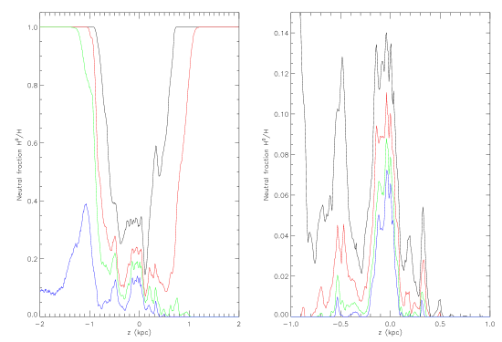
Figure 2: Average neutral fraction as a function of height for ionizing luminosities (left panel) $Q_{49}=0.1$ (black), 0.5 (red), 1 (green), 2 (blue) and (right panel) $Q_{49}=2$ (black), 3 (red), 4 (green), 5 (blue).

In their hydrodynamic simulations of a vertically stratified ISM driven by individual supernova explosions, Joung & Mac Low (2006) find that the density power spectrum peaks at $\sim 20$ pc and that the most energy-containing scales lie at 20-40 pc (see their Fig. 8). On the other hand, they find no single effective driving scale; energy injection occurs over a broad range of scales, with greater than 90% of the total kinetic energy contained in wavelengths shortward of 200 pc. Spatially correlated supernovae explosions that break out of the gaseous disk (i.e., superbubble blow outs) and high-altitude Type Ia supernovae are the main drivers of turbulent motions of the halo gas. These structures have larger characteristic scales (several hundred parsecs) than individual supernova remnants in the disk, due to the higher amount of energy and lower background gas density, respectively; see Fig. 2 of Joung & Mac Low (2006).

For our photoionization simulations we consider a subset of this grid extending to $\pm$2 kpc in $z$. Memory requirements of our photoionization code on current desktop computers required us to re-bin the density grid by a factor of four giving a resolution of 7.8 pc per grid cell. The computationally straightforward approach of running the radiative transfer code in a static realization of the hydrodynamical code is justified by the recombination time scale of $\sim 3$ Myr, much shorter than the dynamical timescale of $\sim 100$ Myr in an 8000 K hydrogen gas with a total number density of $1\textrm{ cm}^{-3}$ and $n_{e}=0.03\textrm{ cm}^{-3}$ (Spitzer, 1978).

Density, velocity, and temperature slices of the simulation are shown in Joung et al. (2009). In Fig. 1 we show the horizontally averaged density as a function of height compared to a model for the hydrogen density in the ISM. The model comprises a Dickey-Lockman (Dickey & Lockman, 1990) distribution for neutral hydrogen with a low density, vertically extended distribution for ionized hydrogen as follows:

$$n(z)=0.4\exp{\left[-\frac{1}{2}\left(\frac{z}{90}\right)^{2}\right]}+0.11\exp{\left[-\frac{1}{2}\left(\frac{z}{225}\right)^{2}\right]}+0.06\exp{\left[-\frac{|z|}{400}\right]}+0.025\exp{\left[-\frac{|z|}{1000}\right]}\;,$$ (1)

where the number density is in units of cm^-3 and the heights, $z$ are in pc. The first three terms represent the density of neutral hydrogen and the fourth term represents ionized hydrogen. The mean vertical column density (within the range $|z|\leq 2\,{\rm kpc}$) for the simulations is in good agreement with that derived from equation 1 with a value of $\sim 7\times 10^{20}\,{\rm cm}^{-2}$. However, the density structure of the dynamical simulation is more centrally peaked than the Galactic model described by equation 1. As we discuss later, this is most likely due to the absence of magnetic fields in the current dynamical simulations.

2.2 Photoionization Simulations

The primary focus of this paper is the ionization structure of hydrogen and the penetration of Lyman continuum photons to large heights above the Galactic midplane. Therefore for the photoionization simulations we use the 3D hydrogen-only Monte Carlo photoionization code described in Wood & Loeb (2000). Because neutral hydrogen is opaque to Lyman continuum radiation whereas the optical depth of nearly fully ionized hydrogen is much lower, we use an iterative process to establish a self-consistent distribution of neutral and ionized hydrogen. This code follows the propagation of ionizing photons within a 3D linear cartesian density grid and accurately computes the 3D ionization structure of hydrogen for an assumed uniform temperature. The code includes photoionization arising from both direct stellar photons and also the diffuse radiation field produced by recombinations to the ground level of hydrogen. We have extended the original Wood & Loeb (2000) code to include the effects of dust scattering and absorption of ionizing photons. We adopt an opacity of $1.3\times 10^{-22}\,{\rm cm}^{-2}\,{\rm H}^{-1}$ appropriate for silicate dust at Lyman continuum wavelengths as discussed in Mathis & Wood (2005), and assume albedo and scattering phase function asymmetry parameters $a=0.5$, $g=0.5$. While dust opacity may influence the ionization structure of high density H II regions, its effects in the low density DIG that we are investigating are not important. We find that typically less than 1% of ionizing photons are absorbed by dust in our simulations. The simulated emission measure distributions in § 3 below do not include regions of the grid with $|z|<150$ pc, thereby further mitigating the effects of dust in our analysis. For our current study we are not investigating emission line ratios, so the single temperature hydrogen-only code is sufficient. It has the advantage of being faster and requiring less memory than our code that computes the ionization structure of many more elements and also the electron temperature (Wood et al., 2004).

The sources of ionizing radiation are point sources within the simulation grid representing single stars or clusters of OB stars. We follow the approach of Ciardi et al. (2002) and randomly choose $x$ and $y$ locations of the sources uniformly within the grid. The $z$ coordinate of each source is randomly chosen from a Gaussian distribution with a scale height of 63 pc (Maíz-Apellániz, 2001).

The catalogue of 424 O stars within 2.5 kpc of the Sun (Garmany et al., 1982) indicates a stellar surface density of 24 stars kpc^-2. The Lyman continuum luminosity from these stars was estimated to be $Q=7\times 10^{51}\,{\rm s}^{-1}$ (Vacca et al., 1996). The density field from the hydrodynamic simulation represents a slice of the ISM with a horizontal width of 500 pc, so adopting the estimated stellar surface density, we would expect around six sources within our grid providing an ionizing luminosity of around $10^{50}\,{\rm s}^{-1}$. A fraction of these ionizing photons will produce the DIG, with the rest producing local H ii regions or escaping from the simulation entirely. We do not consider the formation of high density H ii regions around sources, so our models are really considering the ionizing photons that have escaped from their local environment into the lower density diffuse ISM. In our simulations we therefore select random locations for six ionizing sources. We uniformly distribute the ionizing luminosity among the six sources and investigate total luminosities (i.e., ionizing photons escaping from traditional H ii regions) in the range $0.1\leq Q_{49}\leq 10$, where $Q_{49}=Q/(10^{49}\,{\rm s}^{-1})$, covering a range of scenarios allowing for a lower and higher Lyman continuum budget than estimated by Vacca et al. (1996).

Repeating boundary conditions are adopted for the Monte Carlo radiation transfer whereby ionizing photons that exit an $x$ or $y$ face of the grid are re-injected on the opposite face of the grid with their direction of travel unaltered. This simulates the more realistic situation within the Galaxy of ionizing photons that originate from distant sources. Therefore ionizing photons can only exit through the top or bottom $z$ faces of the grid or if they are degraded to a non-ionizing photon or absorbed by dust.

3 Results

We investigated a large number of models for different source locations and total ionizing luminosities. The position of the sources within the density grid and the total ionizing luminosity affect the vertical extent to which gas in the hydro simulation can be ionized. For some realizations of the randomly sampled source locations, sources may be placed many tens of pc above the midplane, and thus above the densest regions in the hydrodynamic simulation. Such a positioning of sources results in more of the gas at large heights being ionized compared to simulations where the sources are confined to midplane regions. Similar results were found in the ionization simulations of Ciardi et al. (2002) who investigated the escape of ionizing photons from vertically stratified smooth and 3D (fractal) ISM density distributions.

The single parameter that most strongly influenced our results and determined the vertical extent to which the gas could be ionized was the total ionizing luminosity, $Q_{49}$. The number and location of ionizing sources did not have a big effect – if a source was randomly placed within a very dense region of the grid and its ionizing photons were trapped, there were always other sources in less dense regions that could provide the photons to ionize gas at large heights. In the following sections we quantitatively present the results of our photoionization simulations.

3.1 Distribution of neutral and ionized hydrogen

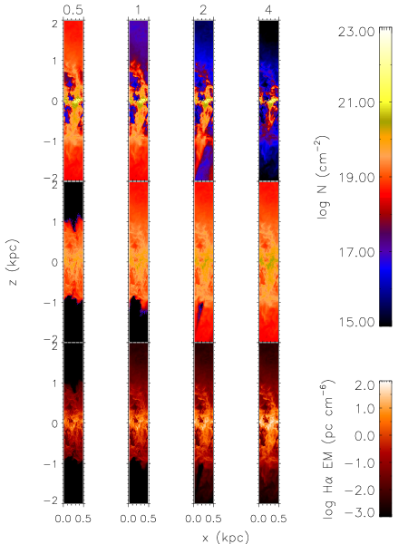
Figure 3: Edge-on visualizations of the simulation grids. Column densities of neutral hydrogen (top row) and ionized hydrogen (middle row), and emission measure ($\int n_{e}^{2}ds$) (bottom row) are shown for ionizing luminosities of (left to right) $Q_{49}=0.5,1,2,4$.

Figure 2 shows the average neutral fraction ($n[{\rm H}^{0}]/n[{\rm H}^{0}+{\rm H}^{+}]$) as a function of height for different ionizing luminosities. At low values of $Q_{49}\lesssim 1$, the grid becomes fully neutral for $|z|\gtrsim 800$ pc. We find that the grid is almost fully ionized at large heights ($|z|\gtrsim 0.5$ kpc) for total ionizing luminosities $Q_{49}\gtrsim 2$. Figure 3 displays the emission measure ($\textrm{EM}\equiv\int n_{e}^{2}ds$) and H I column density maps for edge-on viewing of the grid, showing the development of extended ionized volumes as the ionizing luminosity increases.

To maintain the ionization of the Galactic DIG in the Solar neighborhood (within 2-3 kpc) requires a Lyman continuum flux in the midplane of around $4\times 10^{6}\,{\rm cm}^{-2}\,{\rm s}^{-1}$ (Reynolds, 1990a), about 12% of that available from OB stars (Abbott, 1982; Vacca et al., 1996). The required ionizing luminosity, both for the Galactic DIG and for our simulations, is lower than that estimated to be available from OB stars in the Galaxy and represents Lyman continuum photons that leak out of traditional (high density) H ii regions to ionize the DIG. As discussed in § 2.2, assuming the Vacca et al. (1996) value for the ionizing flux in the solar neighborhood ($3.4\times 10^{7}\,{\rm cm}^{-2}\,{\rm s}^{-1}$), the total flux available to ionize our grid is around $10^{50}\,{\rm s}^{-1}$. In our simulations the gas is ionized at large heights when $Q_{49}\gtrsim 2$, slightly higher than the 12% suggested by Reynolds (1990a).

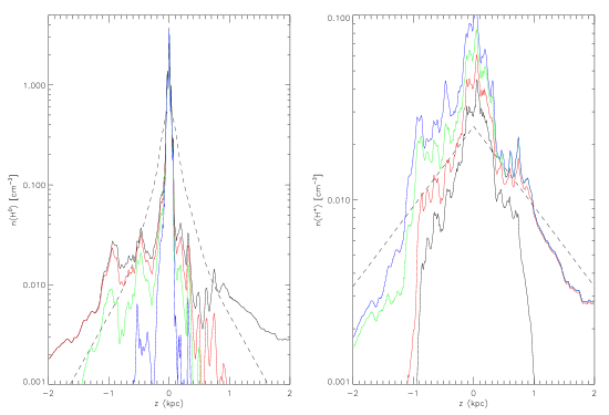
Figure 4: Mean densities of neutral (left panel) and ionized hydrogen (right panel) for ionizing luminosities $Q_{49}=0.5$ (black), 1 (red), 2 (green), 4 (blue). Overplotted with dashed lines are the Dickey-Lockman distribution for neutral hydrogen (left panel) and the average electron density derived for the Galactic DIG (right panel).

Figure 4 shows the average neutral and ionized hydrogen densities as a function of height for the simulation with $Q_{49}=2$. As described above, the mean densities at large $|z|$ are lower than the model of equation 1 for hydrogen density in the Galaxy. Therefore it is not surprising that the mean density of neutral hydrogen for $|z|\gtrsim 200$ pc in the ionization simulations is lower than the Dickey-Lockman distribution. The mean electron density from the simulations is also lower than derived for the DIG in the Galaxy, but does follow an exponential distribution at large $|z|$ with a scale height of around 500 pc. This is smaller than the scale height of the DIG in our Galaxy.

For comparison, we investigated ionization of a smooth density grid with the hydrogen density described by equation 1. In the simulations we adopted an ionizing luminosity $Q_{49}=2$ and multiplied the first three terms in equation 1 by a constant factor until we achieved ionization of the gas at large heights and a total escape fraction of ionizing photons of around 10% through the top and bottom of our grid ($z=\pm 2$ kpc). To achieve this we find that the three components representing the “neutral hydrogen” in equation 1 must be multiplied by about 1/3. This is consistent with the ionization study of Miller & Cox (1993) who found that if they used the known locations of O stars in the solar neighborhood then the hydrogen density within the smooth component must be lower than the Dickey-Lockman distribution to allow gas at large heights to be ionized. Also see the results of 3D simulations by Ciardi et al. (2002) and the discussion in Haffner et al. (2009). For O stars to provide the ionization of the DIG requires a 3D distribution of gas in which the density of any smooth component should be at most one third of the Dickey-Lockman distribution for neutral hydrogen. To make up the remainder of the observed neutral hydrogen requires higher density “clouds” (Miller & Cox, 1993) or denser regions such as produced in a turbulent medium.

We further investigated the survival of neutral clouds at large heights above the midplane and performed simulations to study the ionization of a 50 pc radius spherical blob positioned at $z=1.5$ kpc in the grid. Figure 5 shows a slice through the center of the ionization grid containing a blob of various densities showing the transition from almost fully neutral to fully ionized with decreasing blob density. In our simulations with $Q_{49}=2$, a blob with $n\gtrsim 0.1\,{\rm cm}^{-3}$ remains neutral, except for a very thin ionized skin, not resolvable in our current simulations. Lower density blobs exhibit a thicker ionized skin and become neutral deeper into the blob. The ionized skin is mostly directed towards the midplane, but does extend all around the blob due to photons from the diffuse ionizing radiation field. The number density of neutral hydrogen blobs in our simulations agrees well with density estimates ($0.05\lesssim n\lesssim 0.5$) for high velocity clouds (e. g. Wakker & van Woerden, 1997; Wakker et al., 2008; Hill et al., 2009).

3.2 Emission measure distribution

The results of the previous section demonstrate that the hydrodynamical simulations produce density structures that readily allow for ionizing photons to percolate to high altitudes and produce extended layers of ionized gas. In Figure 6 we present probability distributions of emission measure, ${\rm EM}=\int n_{\rm e}^{2}\,{\rm d}s$, for face-on and edge-on views of the simulation grid. In forming these EM distributions we have removed the contributions from grid cells in the simulation with $|z|<150$ pc, which contain the densest regions of the simulation and in reality should also include high density H II regions. In forming the EM from the simulations we use the computed electron density and not an EM derived from simulated H$\alpha$ observations. An H$\alpha$ derived EM would require an accurate temperature calculation incorporating heating and cooling from a radiation-magnetohydrodynamical simulation, beyond the scope of the current paper.

For comparison we also show EM distributions in the Galaxy derived from subsets of the Wisconsin H-Alpha Mapper (WHAM) Northern Sky Survey (Haffner et al., 2003). The two EM $\sin|b|$ distributions displayed are of high-latitude ($|b|>10^{\circ}$) sightlines that sample 1) all DIG gas north of $\delta=-30^{\circ}$ and 2) the Perseus Arm, which is conveniently separated out in the velocity range $-100\textrm{ km s}^{-1}\lesssim V_{\rm lsr}\leq-25\textrm{ km s}^{-1}$ (Haffner et al., 1999). In both cases, we have excluded the large classical H II regions identified by Hill et al. (2008) to leave a sample consisting primarily of DIG emission.

Figure 6 shows that the simulations produce EM distributions that are broader than observed for the Galactic DIG. In making these comparisons we compare the face-on view of the simulation with the EM distribution for all Galactic sightlines $b>10^{\circ}$, and comparing the edge-on view with the EM distribution for the Perseus Arm. The very extended low EM tail seen in the edge-on view of the simulation grid will be diminished somewhat in H$\alpha$ derived EMs since hot ($T>10^{5}$ K), low density ($n<10^{-2}\,{\rm cm}^{-3}$) gas at high latitudes (see Joung et al., 2009) will have a very low H$\alpha$ emissivity.

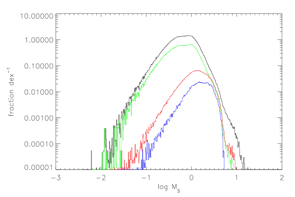
Figure 7: Histograms of sonic Mach number for subsets of the hydrodynamical model. Black line: entire sample. Green line: all gas at $|z|>125\textrm{ pc}$. Red line: all warm (defined as $5000<T/\textrm{K}<20000$) gas. Blue line: warm gas at $|z|>125\textrm{ pc}$. The sound speed in each cell is calculated as $v=7.18\,(T/8000\textrm{ K})^{1/2}\textrm{ km s}^{-1}$, appropriate for a solar metallicity, neutral gas.

The standard deviation of $\log\mathrm{EM}$ in the face-on view of the photoionization simulation is $0.56$. This is much wider than the observed value of $\sigma_{\mathrm{EM}\sin|b|}=0.190$ for the DIG (Hill et al., 2008). Indeed, in the isothermal MHD models presented by Kowal et al. (2007) and Hill et al. (2008), only the highly supersonic models produce such a wide distribution of emission measures. Turbulence in the DIG is likely mildly supersonic, with a Mach number of $1-3$ (Padoan et al., 1997; Hill et al., 2008; Berkhuijsen & Fletcher, 2008). In the hydrodynamical models presented here, the warm gas, defined as $5000\textrm{ K}<T<20000\textrm{ K}$, has a mean sonic Mach number of $M_{s}=1.2-1.7$, as shown in Figure 7.

The breadth of the EM distributions indicates that the hydrodynamical simulations show much larger contrasts between low and high density gas than present in the Galaxy. This result, combined with the average hydrogen density at large heights being lower than derived in the Galaxy (Fig. 1), leads us to speculate that the effects of magnetic fields (not present in the simulation) could reconcile the model with observations. Including magnetic fields in the hydrodynamical simulations will provide two main effects: a higher signal speed, and thus a lower effective Mach number, which will result in less extreme density variations (as seen in the simulations by de Avillez & Breitschwerdt, 2005) and additional pressure support that will levitate and maintain a higher density with height. We anticipate that these combined effects will result in narrower EM distributions and higher densities with height, bringing our simulations closer to observationally derived values for the EM and height dependence of the density of the neutral and ionized gas.

4 Comparison to previous work

The escape fractions of ionizing photons from our simulations are around 10% for $Q=2\times 10^{49}\,{\rm s}^{-1}$ and increase for larger ionizing luminosities, entirely consistent with the study by Ciardi et al. (2002). However, ours and other 3D simulations differ from the 1D model of Bland-Hawthorn & Maloney (1999) that predicted very small ionizing fluxes at small distances above the galactic midplane (see Fig. 6 in Putman et al. 2003). This difference is not surprising for several reasons: the Bland-Hawthorn & Maloney (1999) model considered all ionizing sources to be located in the Galactic midplane and to suffer extinction due to a uniform density slab of dust. This is entirely reasonable for their study of ionization of high velocity clouds at very large distances from the Galaxy, and for HVCs their model predicts appropriate escape fractions and ionizing fluxes. However, for studying photoionization of clouds at small distances from the Galactic plane their model predicts a vanishingly small flux, which is clearly not correct for a 3D simulation. Considering these differences between 1D and 3D models, we believe it is inappropriate to reject photoionization of the Galactic cirrus as a source for at least some of the observed H$\alpha$ emission (Mattila et al., 2007). Indeed, the observed H$\alpha$ intensities of typically 2 Rayleighs from the clouds studied by Mattila et al. (2007) require ionizing fluxes of around $5\times 10^{6}\,{\rm photons}\,{\rm cm}^{-2}\,{\rm s}^{-1}$, well within the range suggested for the Solar neighborhood by Vacca et al. (1996). For a slab cloud with a uniform density of $10\,{\rm cm}^{-3}$ normally illuminated on one side and assuming an ionized gas temperature of 8000 K, the ionized skin would be $\sim 0.05$ pc thick and contribute to the observed H$\alpha$ intensity in addition to any scattered light component. Allowing for a photoionized skin on the surface of these clouds means that the observed H$\alpha$ emission need not be attributed entirely to cosmic rays (del Burgo & Cambrésy, 2006) or scattered light from midplane H ii regions (Mattila et al., 2007).

Recent models of the DIG in M51 (Seon, 2009) suggested that O stars were not capable of producing ionization at large distances from their immediate surroundings. This conclusion was based on an ionization model of a smoothly distributed ISM (uniform slab or an exponential disk) that appeared to show that unrealistically small optical depths of neutral hydrogen in the ISM were required to allow ionizing photons to reach gas at large distances from the O stars. However, the analysis by Seon (2009) did not comprise a correct photoionization simulation where the ionization state of the gas was calculated self-consistently. Instead the penetration of ionizing photons through a neutral ISM was characterized using an $\exp(-\tau)$ factor where $\tau$ is the optical depth due to neutral hydrogen. Seon (2009) correctly stated that the optical depths of neutral hydrogen in a smooth ISM are large and will not allow photons to reach large distances from the midplane. Instead, Seon (2009) claims that optical depths of neutral hydrogen need to be smaller by factors of around $10^{-5}$ to allow ionizing photons to penetrate from midplane O stars to high altitudes in M51. However, in a photoionization simulation the neutral hydrogen fraction in diffuse ionized gas is in fact very low, typically $10^{-3}$ and even smaller closer to ionizing sources (Wood & Mathis, 2004). Therefore when the medium is ionized Lyman continuum photons can indeed penetrate to large distances. In addition, as demonstrated in ours and other simulations clumping of the gas in the ISM produces low density regions and this further helps the ionizing photons reach and ionize gas at large distances from the midplane. The combination of small neutral fractions in the DIG and low density regions in a 3D ISM will combine to produce the low column densities of neutral hydrogen (compared to a smoothly distributed ISM) required for ionizing radiation from O stars to reach and ionize the DIG in M51.

5 Conclusions and future work

Our main conclusion is that the density structures produced by 3D hydrodynamical simulations of a turbulent ISM allow ionizing photons from midplane sources to reach and ionize gas at large altitudes. This is in agreement with previous photoionization simulations of analytically produced fractal density structures that also indicate that a 3D ISM is required for O stars to ionize high altitude gas. We therefore believe that the results of the photoionization simulations of analytic ISM densities and now those of more realistic hydrodynamical simulations lend further compelling support for O stars being the dominant ionization source of the DIG.

While a 3D ISM can solve the problem of propagating ionizing photons to large altitudes, our results indicate that the dynamical simulations likely require additional physics to reproduce the details of the DIG observations within the Galaxy. Compared to the Galactic DIG, the simulations in this paper show broader EM distributions suggesting that magnetic fields may be the missing ingredient to reconcile observations with theory. Magnetic fields will reduce the density variations and provide pressure to support gas and give a higher density at kiloparsec heights above the midplane. This is borne out in the ISM MHD simulations of de Avillez & Breitschwerdt (2005) and preliminary simulations of our own that incorporate magnetic fields (Hill et al. in preparation).

Figure 1: Mean density (solid line) from the hydrodynamic simulations compared with the Dickey-Lockman distribution for neutral hydrogen (dashed line) and a Dickey-Lockman plus extended component representing diffuse ionized gas (dot-dash line).

Figure 5: Neutral fraction as a function of height through the center of the grid for simulations with a 50 pc spherical blob located at 1.5 kpc above the midplane. The ionizing luminosity is $Q_{49}=2\,{\rm s}^{-1}$ and the curves (lowest to highest) are for blob densities of 0.01, 0.05, 0.1, 0.5 cm^-3. As the density increases the blob transitions from being almost fully ionized, to having an ionized surface skin, to being almost fully neutral.

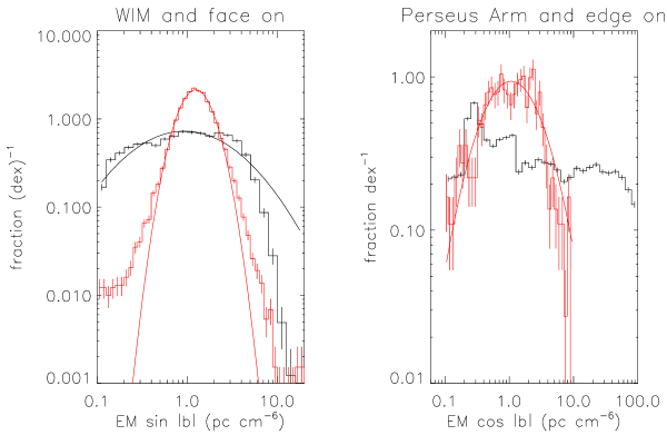
Figure 6: Emission measure distributions for the Galactic DIG from the WHAM survey and from our $Q_{49}=2$ photoionization simulation. Fraction (dex)^-1 is the fraction of points in each bin divided by the logarithmic bin interval. Left panel: The black histogram is of $\int n_{e}^{2}ds$ in the simulation, viewed face-on. The red histogram is of EM $\sin|b|$ from the WHAM survey with classical H II regions and sightlines with $|b|<10^{\circ}$ removed, from Hill et al. (2008). Lognormal fits to each distribution are also shown. Right panel: The black histogram is of $\int n_{e}^{2}ds$ in the simulation, viewed edge-on. The red histogram is of EM $\cos|b|$ from the WHAM survey toward the Persus Arm for velocities in the range $-100\textrm{ km s}^{-1}\lesssim V_{\rm lsr}\leq-25\textrm{ km s}^{-1}$ with classical H II regions removed. For the emission measures from the simulations we have removed contributions from midplane regions with $|z|<150$ pc. Notice that the model distributions are broader than the WHAM observations.

References

- Abbott (1982) Abbott, D. C. 1982, ApJ, 263, 723
- Armstrong et al. (1995) Armstrong, J. W., Rickett, B. J., & Spangler, S. R. 1995, ApJ, 443, 209
- Benjamin (1999) Benjamin, R. 1999, in Interstellar Turbulence, ed. J. Franco & A. Carraminana, 49
- Berkhuijsen & Fletcher (2008) Berkhuijsen, E. M. & Fletcher, A. 2008, MNRAS, 390, L19
- Bland-Hawthorn & Maloney (1999) Bland-Hawthorn, J. & Maloney, P. R. 1999, ApJ, 510, L33
- Boisse (1990) Boisse, P. 1990, A&A, 228, 483
- Chepurnov & Lazarian (2010) Chepurnov, A. & Lazarian, A. 2010, ApJ, 710, 853
- Ciardi et al. (2002) Ciardi, B., Bianchi, S., & Ferrara, A. 2002, MNRAS, 331, 463
- de Avillez & Breitschwerdt (2005) de Avillez, M. A. & Breitschwerdt, D. 2005, A&A, 436, 585
- del Burgo & Cambrésy (2006) del Burgo, C. & Cambrésy, L. 2006, MNRAS, 368, 1463
- Dickey & Lockman (1990) Dickey, J. M. & Lockman, F. J. 1990, ARA&A, 28, 215
- Dove & Shull (1994) Dove, J. B. & Shull, J. M. 1994, ApJ, 430, 222
- Ferguson et al. (1996) Ferguson, A. M. N., Wyse, R. F. G., Gallagher, III, J. S., & Hunter, D. A. 1996, AJ, 111, 2265
- Fryxell et al. (2000) Fryxell, B., Olson, K., Ricker, P., Timmes, F. X., Zingale, M., Lamb, D. Q., MacNeice, P., Rosner, R., Truran, J. W., & Tufo, H. 2000, ApJS, 131, 273
- Gaensler et al. (2008) Gaensler, B. M., Madsen, G. J., Chatterjee, S., & Mao, S. A. 2008, PASA, 25, 184
- Garmany et al. (1982) Garmany, C. D., Conti, P. S., & Chiosi, C. 1982, ApJ, 263, 777
- Gómez et al. (2001) Gómez, G. C., Benjamin, R. A., & Cox, D. P. 2001, AJ, 122, 908
- Haffner et al. (2009) Haffner, L. M., Dettmar, R., Beckman, J. E., Wood, K., Slavin, J. D., Giammanco, C., Madsen, G. J., Zurita, A., & Reynolds, R. J. 2009, Rev. Mod. Phys., 81, 969
- Haffner et al. (1999) Haffner, L. M., Reynolds, R. J., & Tufte, S. L. 1999, ApJ, 523, 223
- Haffner et al. (2003) Haffner, L. M., Reynolds, R. J., Tufte, S. L., Madsen, G. J., Jaehnig, K. P., & Percival, J. W. 2003, ApJS, 149, 405
- Hill et al. (2008) Hill, A. S., Benjamin, R. A., Kowal, G., Reynolds, R. J., Haffner, L. M., & Lazarian, A. 2008, ApJ, 686, 363
- Hill et al. (2009) Hill, A. S., Haffner, L. M., & Reynolds, R. J. 2009, ApJ, 703, 1832
- Hood et al. (2008) Hood, B., Wood, K., Seager, S., & Collier Cameron, A. 2008, MNRAS, 389, 257
- Joung & Mac Low (2006) Joung, M. K. R. & Mac Low, M. 2006, ApJ, 653, 1266
- Joung et al. (2009) Joung, M. R., Mac Low, M., & Bryan, G. L. 2009, ApJ, 704, 137
- Kowal et al. (2007) Kowal, G., Lazarian, A., & Beresnyak, A. 2007, ApJ, 658, 423
- Kuijken & Gilmore (1989) Kuijken, K. & Gilmore, G. 1989, MNRAS, 239, 605
- Maíz-Apellániz (2001) Maíz-Apellániz, J. 2001, AJ, 121, 2737
- Mathis & Wood (2005) Mathis, J. S. & Wood, K. 2005, MNRAS, 360, 227
- Mattila et al. (2007) Mattila, K., Juvela, M., & Lehtinen, K. 2007, ApJ, 654, L131
- Miller & Cox (1993) Miller, W. W. I. & Cox, D. P. 1993, ApJ, 417, 579
- Padoan et al. (1997) Padoan, P., Jones, B. J. T., & Nordlund, A. P. 1997, ApJ, 474, 730
- Putman et al. (2003) Putman, M. E., Bland-Hawthorn, J., Veilleux, S., Gibson, B. K., Freeman, K. C., & Maloney, P. R. 2003, ApJ, 597, 948
- Rand (1998) Rand, R. J. 1998, Publications of the Astronomical Society of Australia, 15, 106
- Reynolds (1989) Reynolds, R. J. 1989, ApJ, 339, L29
- Reynolds (1990a) —. 1990a, ApJ, 349, L17
- Reynolds (1990b) —. 1990b, ApJ, 348, 153
- Reynolds (1991) Reynolds, R. J. 1991, in IAU Symposium, Vol. 144, The Interstellar Disk-Halo Connection in Galaxies, ed. H. Bloemen, 67–76
- Reynolds et al. (1999) Reynolds, R. J., Haffner, L. M., & Tufte, S. L. 1999, ApJ, 525, L21
- Savage & Wakker (2009) Savage, B. D. & Wakker, B. P. 2009, ApJ, 702, 1472
- Selkowitz & Blackman (2007) Selkowitz, R. & Blackman, E. G. 2007, MNRAS, 382, 1119
- Seon (2009) Seon, K. 2009, ApJ, 703, 1159
- Shaviv (2000) Shaviv, N. J. 2000, ApJ, 532, L137
- Spitzer (1978) Spitzer, L. 1978, Physical processes in the interstellar medium (New York: Wiley)
- Vacca et al. (1996) Vacca, W. D., Garmany, C. D., & Shull, J. M. 1996, ApJ, 460, 914
- Wakker & van Woerden (1997) Wakker, B. P. & van Woerden, H. 1997, ARA&A, 35, 217
- Wakker et al. (2008) Wakker, B. P., York, D. G., Wilhelm, R., Barentine, J. C., Richter, P., Beers, T. C., Ivezić, Ž., & Howk, J. C. 2008, ApJ, 672, 298
- Wolfire et al. (1995) Wolfire, M. G., Hollenbach, D., McKee, C. F., Tielens, A. G. G. M., & Bakes, E. L. O. 1995, ApJ, 443, 152
- Wood & Loeb (2000) Wood, K. & Loeb, A. 2000, ApJ, 545, 86
- Wood & Mathis (2004) Wood, K. & Mathis, J. S. 2004, MNRAS, 353, 1126
- Wood et al. (2004) Wood, K., Mathis, J. S., & Ercolano, B. 2004, MNRAS, 348, 1337