Scalable distributed service migration via Complex Networks Analysis

Abstract

With social networking sites providing increasingly richer context, User-Centric Service (UCS) creation is expected to explode following a similar success path to User-Generated Content. One of the major challenges in this emerging highly user-centric networking paradigm is how to make these exploding in numbers yet, individually, of vanishing demand services available in a cost-effective manner. Of prime importance to the latter (and focus of this paper) is the determination of the optimal location for hosting a UCS. Taking into account the particular characteristics of UCS, we formulate the problem as a facility location problem and devise a distributed and highly scalable heuristic solution to it.

Key to the proposed approach is the introduction of a novel metric drawing on Complex Network Analysis. Given a current location of UCS, this metric helps to a) identify a small subgraph of nodes with high capacity to act as service demand concentrators; b) project on them a reduced yet accurate view of the global demand distribution that preserves the key attraction forces on UCS; and, ultimately, c) pave the service migration path towards its optimal location in the network. The proposed iterative UCS migration algorithm, called cDSMA, is extensively evaluated over synthetic and real-world network topologies. Our results show that cDSMA achieves high accuracy, fast convergence, remarkable insensitivity to the size and diameter of the network and resilience to inaccurate estimates of demands for UCS across the network. It is also shown to clearly outperform local-search heuristics for service migration that constrain the subgraph to the immediate neighbourhood of the node currently hosting UCS.

I Introduction

One of the most significant changes in networked communications over the last few years concerns the role of the end-user. Till recently the end-user has been the consumer of content and services generated by explicit entities called content and service providers, respectively. Nowadays, the Web2.0 technologies have resulted in/enabled a paradigm shift towards more user-centric approaches to content generation and provision. The first strong evidence of this shift has been the abundance of User-Generated Content ($UGC$) in social networking sites, blogs, wikis, or video distribution sites such as YouTube, which motivated even the rethinking of the Internet architecture fundamentals [1], [2]. The generalization of the $UGC$ concept towards services is increasingly viewed as the next major trend in user-centric networking [3].

The user-oriented service creation concept aims at engaging end-users in the generation and distribution of service components, more generally service facilities [4]. To facilitate the wide proliferation of the so-called User-Generated Service ($UGS$) paradigm, some key technical challenges should be addressed such as a) the design of simple programming interfaces that will enable the involvement of end-users without strong programming background; and b) the deployment of scalable distributed mechanisms for discovering, publishing, and moving service facilities within the network.

Our work focuses on the second challenge. In particular, it addresses the problem of optimally placing service facilities within the network so that the cost of accessing and using them is minimized. The problem is typically viewed as an instance of the family of facility location problems and is formulated as an $1$- or, more generally, $k$-median problem, depending on whether facilities can be replicated in the network [5]. The main bulk of proposed solutions to the problem are centralized (see, for instance, [6]): the optimal service location is determined by a single entity that possesses global information for both the network topology and distribution of service demand across the network. Nevertheless, the service deployment scenarios considered in this work, involving the flexible and scalable deployment of many distributed user-generated services within possibly large networks, bring traditional centralized approaches to the problem solution to their limits. Gathering the required information to a single physical location is already a challenge. Furthermore, the centralized treatment of the problem assumes the existence of an ideal super node bearing the burden of decision-making. This burden is primarily due to the computationally intensive $1(k)$-median problem [5]. Given that (minor) user demand shifts or network topology changes may alter the optimal service location, it is neither practical nor affordable to each time centrally compute a new problem solution.

In our paper we propose solutions for overcoming these limitations. The approach we have taken is highly decentralized; the service facilities migrate from the node that makes them available towards the minimum-cost location by traversing a cost-decreasing path. It is also scalable; similar to other proposals in literature, it moves the service facilities in the network by iteratively solving locally a much smaller scale 1(k)-median optimization problem than what a global centralized solution would require. Nevertheless, it departs from standard practices in the way it selects the nodes for the local 1(k)-median problem. State-of-the-art approaches (for example, [7, 8]) recruit those nodes from their immediate local neighborhood. On the contrary, our algorithm invests additional effort to make a more informed selection of these nodes, which promotes the “correct" directions of migration towards the globally optimal locations.

To achieve this, we devise a metric, called weighted Conditional Betweenness Centrality (wCBC), that draws on Complex Network Analysis (CNA). CNA provides a theoretical framework for unified modeling and analysis of several types of networks and the expectations in the networking community are that its insights could benefit the design of more efficient network protocols. In our work, the CNA-inspired metric helps the service migrate through the network both faster and towards better service locations.

Figure 1: Looking for the next service migration hop: local-search heuristics(left) vs. cDSMA(right).

In each service migration step, the metric serves two purposes. Firstly, it identifies those nodes that contribute most to the aggregate service access cost and pull the service strongly in their direction; namely, nodes that hold a central position within the network topology and/or route large amounts of the demand for it. Secondly, it correctly projects the attraction forces these nodes exert to the service upon the current service location and facilitates a migration step towards the optimal location (Fig. 1). It is really tempting to draw an analogy between our mechanism and a directional antenna: through the directed search (main radiation lobes) the mechanism amplifies the impact of the major service demand attractors (signal sources) while suppressing less important demand poles (noise) that blind local search (omnidirectional antenna) would induce.

We detail the metric and our algorithm, hereafter called cDSMA, in Sections III and IV, respectively, and evaluate them extensively in Section IV. When running over real-world ISP topologies, the cDSMA achieves remarkably high accuracy and fast convergence even when the $1$-median problem iterations are solved locally with very few nodes, less than ten. Moreover, the cDSMA performance is practically invariable with the network size and diameter as well as the spatial dynamics of the service demand distribution across the network. Compared with distributed local-search policies, cDSMA yields consistently better service placements, which are not dependent on the location of the service generation. We summarize our findings, discuss practical implementation aspects of our mechanism, and sketch possible extensions to this work in Section VIII.

II Service placement: a facility location problem

The optimal placement of service facilities in some network structure has been typically tackled as an instance of the facility location problem [5]. Input to the problem is the topology of the network nodes that may host services and/or network users. The objective is to place services in a way that minimizes the aggregate cost of accessing them over all network users.

More precisely, the network topology is represented by an undirected connected graph $G(V,E)$, where $V$ is the set of nodes and $E$ is the set of edges(links) connecting them. Without loss of generality, we assume that all links have a unit weight and thus the minimum cost path $d(n,m)$ between nodes $n$ and $m$, corresponds to the minimum hop count path linking $n$ and $m$. Each network node $n$ serves users that access the service with different intensity(frequency), generating an aggregate demand $w_{n}$ for the service. When there are $k$ service facilities available, the problem of their optimal placement in the network can be formulated as the classical k-median problem; namely, the set $\mathcal{F}$ of $k$ nodes ($|\mathcal{F}|=k$) that are selected to host service facilities minimize the aggregate service access cost:

$$Cost(\mathcal{F})=\sum_{n\in\mathcal{V}}w(n)\cdot\underset{x_{j}\in\mathcal{F}}{\operatorname{min}}\{d(x_{j},n)\}$$ (1)

where $min\{d(x_{j},n)\}$ denotes the distance between each node $n$ and its closest service host node $x_{j}\in\mathcal{F}$. In this paper we focus our attention to the single service facility scenario, $|\mathcal{F}|=1$. Practically, service facilities migrate across the whole network seeking their optimal placement without the possibility for replication. The $1$-median formulation matches better the expectations about the User-Generated Service paradigm, i.e.,many different services generated in various places in the network raising small-scale interest so that replication of their facilities be less attractive. The respective 1-median problem formulation, minimizing the access cost of a service located at node $k\in V$ is given by:

$$Cost(\mathcal{F})=\sum_{n\in\mathcal{V}}w(n)\cdot d(k,n)$$ (2)

In general topologies, optimization problems such as 1-median and $k$-median, are NP-hard requiring global information about the network topology and generated demand load [9]. Thus, so far the main bulk of relevant theoretical work is in the field of approximation algorithms, where various techniques have been applied [11].

II-A Exploiting CNA to overcome limitations

We make use of Complex Network Analysis (CNA) to dramatically reduce the scale of the 1-median problem that network nodes need to solve. We introduce a metric, called Weighted Conditional Betweenness Centrality (wCBC), which draws on a known CNA metric (Betweenness Centrality [12]) and assesses the value of nodes as candidate hosts of the service. The nodes with the highest $wCBC$ values induce a small subgraph on the original network graph, wherein the original optimization problem can be solved more efficiently for the next-best service location in the network. Besides identifying the highest-value nodes for hosting the service, the metric directly lets us map the demand of the rest of the network nodes on this subgraph. We introduce our metric in Section III, whereas the demand mapping process and the overall algorithm are detailed in Section IV.

A similar decentralized approach to the service placement problem was taken by Smaragdakis et al.in [8], although they allow for service replication. Compared to our approach, the authors practically fix a-priori the $k$ $1$-median subgraphs to the $R$-hop neighborhood of the current service locations. Intuitively, small values of $R$, in the order of one or two, ease information gathering but slow down the migration process. We show later in Section VI-D that this local-search approach also adds “noise” to the algorithm’s effort to push the service towards the optimal location in the network. As a result, the algorithm may be trapped in locally anticipated as optimal, yet globally suboptimal, locations. On the contrary, our metric exploits CNA insights to naturally extract a more informed 1-median subgraph and drive us faster towards the optimal service location. We elaborate on how the two approaches relate in Section VI-D.

III Weighted Conditional Betweenness Centrality

Central to our distributed approach is the Weighted Conditional Betweenness Centrality ($wCBC$) metric. It originates from the well-known betweenness centrality metric and captures both topological and service demand information for each node.

III-A Capturing network topology: from BC to CBC

Betweenness centrality, one of the most frequently used metrics in CNA, reflects to what extent a node lies on the shortest paths linking other nodes. Let $\sigma_{st}$ denote the number of shortest paths between any two nodes $s$ and $t$ in a connected graph $G=(V,E)$. If $\sigma_{st}(u)$ is the number of shortest paths passing through the node $u\in$V, then the betweenness centrality index of node u is given by (3).

$$BC(u)=\sum_{s=1}^{|V|}\sum_{t=1}^{s-1}\frac{\sigma_{st}(u)}{\sigma_{st}}$$ (3)

$BC(u)$ captures the ability of a node $u$ to control or assist the establishment of paths between pairs of nodes. It is an average value estimated over all network pairs. In earlier work  [13], we proposed Conditional BC (CBC), as a way to capture the topological centrality of a random network node with respect to a specific node $t$, which in our context is a node visited by the service on its way towards the optimal location. It is defined as

$$CBC(u;t)=\sum_{s\in V,u\neq t}\frac{\sigma_{st}(u)}{\sigma_{st}}$$ (4)

with $\sigma_{st}(s)=0$.

Note that the summation is over all node pairs ($x,t$) $\forall x\in V$ destined at node $t$ rather than all possible pairs, as in (3). Effectively, CBC assesses to what extent a node $u$ acts as a shortest path aggregator towards the current service location $t$ by enumerating the shortest paths to $t$ involving $u$ from all other network nodes.

III-B Capturing service demand: from CBC to wCBC

In general, a high number of shortest paths through the node $u$ does not necessarily mean that equally high demand load stems from the sources of those paths. Naturally, we need to enhance the pure topology-aware $CBC$ metric in a way that it takes into account the service demand that will be eventually served by the shortest paths routes towards the service location. To this end, we introduce weighted conditional betweenness centrality ($wCBC$), where the shortest path ratio of $\sigma_{st}(u)$ to $\sigma_{st}$ in Eq. (4), is modulated by the demand load generated by each node $s$.

$$wCBC(u;t)=\sum_{s\in V,u\neq t}w(s)\cdot\frac{\sigma_{st}(u)}{\sigma_{st}}.$$ (5)

Note that $\sigma_{ut}(u)=\sigma_{ut}$; hence, for each network node $u$, its $wCBC(u;t)$ value is lower bounded by its own demand $w(u)$.

Therefore, $wCBC$ assesses to what extent a node can serve as demand load concentrator towards a given service location. It is straightforward to see that when a service is equally requested by all nodes in the network (uniform demand) the $wCBC$ metric degenerates to the CBC one, within a scale constant.

III-C Metric computation for regular network topologies

Closed-form expressions for $wCBC$ are not easy to obtain except for scenarios with uniform demand and regular topologies. The following two Propositions provide the closed-form expressions for CBC, i.e.,$wCBC$ for $w_{n}=1,~{}\forall n\in V$, in two instances of regular network topologies, the ring and the two-dimensional (2D) grid.

Proposition III.1

In a ring network of $N$ nodes, the CBC value of a node $u$ with respect to another node $t$ are given by:

$$CBC_{ring(N)}(u;t)=\begin{cases}\lceil\frac{N-1}{2}-d(u,t))\rceil^{+}~{}~{}~{}N=2k\\ \lceil\frac{N+1}{2}-d(u,t))\rceil^{+}~{}~{}~{}N=2k+1,~{}k\in Z\end{cases}$$

where $\lceil x\rceil^{+}=max(x,0)$ and $d(u,t)$ is the minimum hop count distance between nodes $u$ and $t$ along the ring.

Proposition III.2

Consider a $M$x$N$ rectangular grid network, where nodes are indexed inline with their position in the grid, i.e.,node $(i,j)$ is the node located at the $i^{th}$ row and $j^{th}$ column of the grid. The CBC value of node $u$ at position $(a,b)$ with respect to node $t$ at position $(k,l)$ is given by (6).

Figure 2: Conditional Betweenness Centrality in regular topologies.

$$CBC_{grid(M,N)}(u;t)=\sum_{i=1}^{M}\sum_{j=1}^{N}\frac{\binom{|b-j|+|a-i|}{|a-i|}\binom{|l-b|+|k-a|}{|k-a|}}{\binom{|l-j|+|k-i|}{|k-i|}}1{\hskip-2.5pt}\hbox{I}_{\{|l-j|+|k-i|==|b-j|+|a-i|+|l-b|+|k-a|\}}$$ (6)

Proof:

The proof of the first proposition is straightforward. There is one minimum hop count path between all pairs of nodes in the ring. The only exception concerns nodes $N/2$ positions away the one from another in rings with even number of nodes, where there are two shortest paths. For given destination node $t$, the $CBC(u,t)$ value is only increased by those shortest paths that encompass the intermediate node $u$. Due to the ring symmetry, their number only depends on the distances between nodes $u$ and $t$ and decreases by one for each additional hop away from $t$. Summing them over the respective half of the ring, yields the result.

For the 2D grid, the problem degenerates into the enumeration of shortest paths between two grid nodes. The denominator of (6) expresses the number of shortest paths between two arbitrary nodes $(row,column)$ coordinates $(i,j)$ and $(k,l)$, whereas the numerator of (6) equals the number of those paths going through a node with coordinates $(a,b)$. We then sum the ratios over all grid nodes with shortest paths to node $t=(k,l)$ encompassing node $u=(a,b)$. ∎

IV The cDSM Algorithm description

In this section we present our CNA-driven Disributed Service Migration Algorithm for the service placement process. The service migration to the optimal location in the network evolves within a finite number of iterations, as we show later in Section IV-B, through a path that continuously decreases the aggregate cost of service access over all network nodes.

IV-A Detailed algorithm description

A single algorithm iteration involves a number of discrete steps. We discuss them below while providing pointers to the algorithm’s pseudocode.

Step 1: Initialization. The algorithm execution starts at the node $s$ that initially deploys the service. The cost of the service placement at node $s$ is assigned an infinite value $(line~{}3)$ to secure the first algorithm iteration $(line~{}11)$. This step is only relevant to the first algorithm iteration.

Step 2: Metric computation and 1-median subgraph derivation. Next, the computation of $wCBC(u;s)$ metric takes place for every node $u$ in the network graph $G(V,E)$. Nodes featuring the top $\alpha\%~{}wCBC$ values together with the node $Host$ currently hosting the service form the subgraph $G_{Host}^{i}$ ($i$ enumerates the algorithm iterations), over which the 1-median problem will be solved $(lines~{}4-5~{}and~{}14-15)$. Clearly, the size of this subgraph and the complexity in the problem solution are directly affected by the choice of the parameter $\alpha$. We show in Section V, that even with very small $\alpha$ values, our algorithm yields solutions very close to the optimal.

Step 3: Mapping the demand of the remaining nodes on the subgraph. In this step, the service demand from nodes in $G\setminus G_{Host}^{i}$ is mapped to the nodes of the $G_{Host}^{i}$ subgraph that explicitly participate in the $1$-median problem solution. How this is done is described in detail in section IV-C. For the moment, it suffices to say that the demand factors $w(n)$ in Eq. (2) are effective demands, $w_{eff}(n;Host)$, dependent on the current service host. They include not only the demands of the nodes selected in the previous step due to their high $wCBC$ values but also the demands of the remaining nodes that are not directly considered in the 1-median problem formulation.

Step 4: 1-median problem solution and service migration to the new host node. Any centralized technique may be used to solve this small-scale optimization problem. Successively better algorithms have been designed during the last few years [11] and one can seek for the best heuristic method available to maximize scalability. The optimization’s outcome is the location of the candidate new Host node, which results in minimum service access cost $C(Host)$ among the nodes of the current subgraph. We assign the value of this cost to the variable $C_{next}$ and test whether it is smaller than $C_{current}$. As long as the condition for cost decrease holds, the service is being relocated to this node, the algorithm iterates again through steps 2-4, and the service continues its progress towards the (globally) lowest-cost location.

Algorithm 1 cDSMA in G(V,E)

1.  $choose\ randomly\ node\ s$

2.  $place\ SERVICE\ @\ s\$

3.  $C_{current}\leftarrow\infty$

4.  $\textbf{for all}\ u\in G\ \textbf{do}\ compute\ wCBC(u;s)$

5.  $G_{s}^{o}\leftarrow\{\alpha\%\ of\ G\ with\ top\ wCBC\ values\}\cup\{s\}$

6.  $\textbf{for all}\ u\in G_{s}^{o}\ \textbf{do}$

7.  $\ \ \ compute\ w_{map}(u;s)$

8.  $\ \ \ w_{eff}(u;s)\leftarrow w_{map}(u;s)+w(u)$

9.  $Host\ \leftarrow\textit{1-median}\ solution\ in\ G_{s}^{o}$

10.  $C_{next}\leftarrow C(Host),~{}i\leftarrow 1$

11.  while $C_{next}<C_{current}$ do

12.     $move\ SERVICE\ to\ Host$

13.     $C_{current}\leftarrow C_{next}$

14.     $\textbf{for all }\ u\in G\ \textbf{do}\ compute\ wCBC(u;Host)$

15.     $G_{Host}^{i}\leftarrow\{\alpha\%\ of\ G\ with\ top\ wCBC\ values\}\cup\{Host\}$

16.     $\textbf{for all}\ u\in G_{Host}^{i}\ \textbf{do}$

17.     $\ \ \ compute\ w_{map}(u;Host)$

18.     $\ \ \ w_{eff}(u;Host)\leftarrow w_{map}(u;Host)+w(u)$

19.     $NewHost\leftarrow\textit{1-median}\ solution\ in\ G_{Host}^{i}\$

20.     $Host\leftarrow NewHost$

21.     $C_{next}\leftarrow C(NewHost),~{}i\leftarrow i+1$

22.  end while

IV-B On the convergence of the proposed algorithm

In this paragraph we study the convergence of cDSMA, showing that the migration process terminates after a finite number of steps. The following lemma serves as the basis for the proof of the convergence proposition.

Lemma 1

A service facility following the migration process of Algorithm 1 will visit at most one network node twice.

Proof:

Assume that the service, initially deployed at some node $n\in G$ reaches the node $b\in G$ twice. Right after its first placement at $b$ upon iteration, say, $i-1$ we solve the 1-median in the subgraph $G_{b}^{i}$ that is formed by the nodes with the top $\alpha\%~{}wCBC(u;b)$ values. Let the corresponding cost be $C_{b}^{i}$. When the service returns to $b$ at iteration, say, $j$ given that the network topology remains the same, the deterministic $wCBC$ criterion of (5) singles out the same subgraph with the one of the first visit, so we have that $G_{b}^{i}=G_{b}^{j}$, implying for the costs that $C_{b}^{i}=C_{b}^{j}$; the cost-decreasing condition of cDSMA is then not fulfilled and, thus, the service locks at node $n$ and the migration process halts. ∎

Proposition IV.1

cDSMA converges at some solution in $O(|V|)$ steps.

Proof:

As stated above, the solution derived from cDSMA is either the globally optimal (best case) or one locally anticipated as lowest-cost solution. Since the number of network nodes is finite, the migrating service will -according to Lemma 1- visit at most every node once and only one of them, twice. This takes $O(|V|+1)=O(|V|)$ steps. ∎

IV-C Mapping the demand of remaining nodes

Besides being the basis for extracting the 1-median subgraph $G_{Host}^{i}$ in each algorithm iteration, the $wCBC$ metric also eases the mapping of the demand that the rest of the network nodes in $G\backslash G_{Host}^{i}$ induce on the 1-median subgraph. This demand must be taken into account when solving the 1-median problem. We do this by modulating the original $wCBC$ metric in accordance with two observations.

Firstly, during the computation of the node $wCBC$ values, the demand of a node $z$ in $G\backslash G_{Host}^{i}$ is taken into account in all the $G_{Host}^{i}$ nodes that lie on the shortest path(s) of $z$ towards the service host node $t$. Simply mapping the demand of $z$ on all those nodes inline with the original $wCBC$ metric, has two shortcomings: (a) when the demand of heavy-hitter nodes is distributed among multiple nodes, any strong direction(gradient) of heavy demand that would otherwise “pull” the service towards a certain direction, tends to fade out; (b) the cumulative demand that is mapped on all $G_{Host}^{i}$ nodes ends up exceeding considerably the real demand a node poses for the service. For example, in Fig. 3 let w(16)= $\delta$; then naive reuse of the $wCBC$ values for service demand mapping would result in nodes $11$, $8$ and $12$ receiving 100%, 50% and 50% of the original $\delta$ demand, respectively. Hence, to achieve accurate mapping, the influence of $z$ should be “credited” only to the first $G_{Host}^{i}$ node encountered on each shortest path from $z$ towards the service host. The set of all these entry nodes $v$ with this property forms a subgraph of $G_{Host}^{i}$.

Secondly, it happens frequently that the shortest paths originating from the 1-median subgraph nodes include further subgraph nodes. The demand of those nodes have to be subtracted when computing the effective demand, with which each $G_{Host}^{i}$ node participates in the solution of the 1-median problem since they are accounted for directly through the very same nodes that generates them.

Mathematically speaking, the weights $w(n)$ in Eq. (2) can be regarded as effective demands

$$w_{eff}(n;Host)=w(n)+w_{map}(n;Host)$$ (7)

that bring together two terms. The first one is the native demand for the service coming from users that are served by node $n$. The second term corresponds to the contribution of the nodes in $G\backslash G_{Host}^{i}$ (i.e.,the non-shaded nodes in Fig. 3), which is given by:

$$w_{map}(n;t) = \sum_{s\in\{G\setminus G_{Host}^{i}\}}w(s)\frac{\sigma^{\prime}_{st}(n)}{\sigma_{st}}$$ (8)

$$\sigma^{\prime}_{st}(n) = \sum_{j=1}^{\sigma_{st}}1{\hskip-2.5pt}\hbox{I}_{\{n~{}\in~{}SP_{st}(j)\bigcap n=\underset{u\in SP_{st}(j)}{\operatorname{argmin}}d(s,u)\}}$$

where $SP_{st}(j)$ is the set of shortest paths from node $s$ to node $t$.

Figure 3: The 1-median subgraph for an example network of 17 nodes with node 7 storing the service facilities in the $i^{th}$ algorithm iteration. There are two non-zero demand mapping terms, $w_{map}(8;7)$ and $w_{map}(11;7)$.

Back to our example in Fig. 3, the nodes $14$, $15$, $16$ and $17$ will now contribute to the $w_{map}(11;7)$ value, whereas the included in $G_{7}^{i}$, node $13$, will not.

V Evaluation methodology

It should have become clear by this point that both the $wCBC$ metric and the performance of cDSMA are heavily dependent on two factors: the network topology and the service demand distribution within the network. Their combination may enforce or, on the contrary, suppress strong service demand attractors and assist (resp. impede) the progress of the service facilities towards their optimal location in the network. In what follows, we study the behavior of cDSMA over a broad set of scenarios that cover efficiently the $\{net~{}topology,demand~{}distribution\}$ variation space.

V-1 Network topology

We consider both synthetic and realistic network topologies. The two synthetic topologies we experiment with are the Barabási-Albert [16] and two-dimensional rectangular grid graphs. The two types of graph models bear very different and distinct structural properties. The B-A graphs form pure probabilistically and can reproduce a highly skewed node degree distribution that approximates the power-law shape reported in literature [17]. Grids, on the other hand, exhibit strictly regular structure with constant node degree and diameter that grows exponentially with the number of network nodes. The synthetic network topologies let us assess the algorithm and highlight its behavior under certain extreme yet predictable operational conditions. Nevertheless, the ultimate assessment of our algorithm is carried out over real-world ISP network topologies. The dataset we consider  [18] has been recently made publicly available [19, 20]. It includes topology data from 850 distinct snapshots of 14 different AS topologies, corresponding to five Tier-1, five Transit and four Stub ISPs. The data were collected daily during the period 2004-08 with the help of a multicast discovering tool called mrinfo. The tool uses IGMP [21] messages to recursively probe all IPv4 multicast-enabled routers and receive back all their multicast interfaces as well as the IP addresses of their neighboring routers. At a second step, the borders between ASes are delimited with application of two mapping mechanisms: firstly, an IP-to-AS mapping for assigning a number to each AS and, secondly, a router-to-AS mapping, via both probabilistic and empirical rules, for assigning each router (having multiple IP addresses) to the “correct” AS. The method can discover connections through L2 switches and turns out to be providing an accurate view of the network topology, circumventing the complexity and inaccuracy of more conventional measurement tools such as traceroute.

V-2 Service demand distribution

Our assessment, at first level, distinguishes between uniform and non-uniform demand scenarios. Uniform demand scenarios are far from realistic; yet they let us study the exclusive impact of network topology upon the behavior of the algorithm. On the contrary, under non-uniform demand distributions, we assess the algorithm under the simultaneous influence of network topology and service demand dynamics. Mathematically speaking, a Zipf distribution models the preference $w(n;s,N)$ of nodes $n,n\in\mathcal{N}$ to a given service

$$w(n;s,N)=\frac{1/n^{s}}{\sum_{l=1}^{N}{1/l^{s}}}.$$ (9)

Practically, the distribution could correspond to the normalized request rate for a given service by each network node. Increasing the value of the parameter $s$ from $0$ to $\infty$, the distribution asymmetry grows from zero (uniform demand) towards higher values.

At a second level, we consider two options as to how the non-uniform service demand emerges spatially within the network. In the default option, each node randomly generates demand according to the Zipf law. The alternative is to introduce geographical correlation by concentrating nodes with high demand in the same network area. This second scenario lends itself to modelling services with strongly local scope; whereas, the first one matches better services that attract geographically broader interest.

V-3 Algorithm performance metrics

We are concerned with two metrics when assessing the performance of cDSMA. The first one relates to its accuracy and denotes the degree of convergence of our heuristic solution to the optimal one, as derived by using ideal global topology and demand information. It is defined as the average normalized excess cost, $\beta_{alg}$, and equals the ratio of the service access cost our algorithm achieves, $C_{alg}(G,\overline{w})$, over the cost achieved with the optimal solution, $C_{opt}(G,\overline{w})$, for given network topology $G$ and service demand distribution $\overline{w}$:

$$\beta_{alg}(\alpha;G,\overline{w})=E[\ \frac{C_{alg}(\alpha;G,\overline{w})}{C_{opt}(\alpha;G,\overline{w})}\ ]$$ (10)

Clearly, $\beta_{alg}$ depends on the percentage $\alpha$ of the network nodes participating in the solution. Generally, the error induced by our heuristic decreases for larger $1$-median subgraphs, i.e.,greater $\alpha$ values. Closely related to $\beta_{alg}$ and its variation are the indices $\alpha_{\epsilon}$, corresponding to the minimum values of $\alpha$, where the access cost achieved with our heuristic algorithm falls within $100\cdot\epsilon\%$ of the optimal.

$$\alpha_{\epsilon}=argmin~{}\{\alpha|\beta_{alg}(\alpha)\leq\ (1+\epsilon)\}$$ (11)

The second metric is the migration hop count, $h_{m}$, which is generally a function of the percentage $\alpha$ and reflects how fast the algorithm converges to its (sub)optimal solution–the question of whether it does so has been answered in Section IV. Smaller $h_{m}$ values imply faster service deployment and less overhead involved to transport and service set-up/shut-down tasks.

For any chosen configuration of the involved parameters, we repeat 20 simulation runs to achieve statistical significance. Typically, the results plotted hereafter are average values together with the 95% confidence intervals, estimated over the 20 runs.

VI Simulation results

VI-A Synthetic topologies: experiments under uniform demand

As already explained in Section V, these experiments demonstrate how different topologies may facilitate or encumber our algorithm. All nodes posing the same demand, the optimal service location coincides with the node featuring the minimum reciprocal of closeness centrality [22].

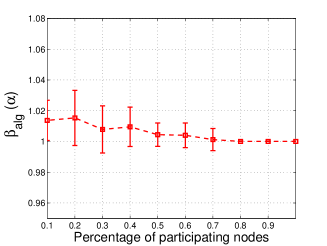
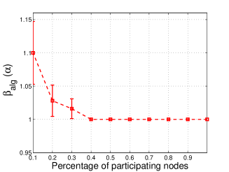
Figure 4: cDSMA accuracy for 10x10 nodes B-A graphs(left) and grids(right) as a function of the 1-median subgraph size: uniform service demand distribution.

Figure 4 plots the average normalized excess cost $\beta_{alg}$ for B-A and grid graphs of 100 nodes. Qualitatively, the two plots are similar: the error induced by our heuristic decreases monotonically with the 1-median subgraph size. However, both starting values, $\beta_{alg}(0.1)$, and the required subgraph size for achieving optimal performance, $\alpha_{0}$, differ. The behavior of cDSMA on the B-A graph is better. The aggregate service access cost increase is within $2\%$ of the optimal, even when we include $10\%$ of network nodes in the 1-median problem solution. On the contrary, reaching similar accuracy for the grid would require, on average, no less that $40\%$ of the network nodes.

Both grids and B-A graphs have structured connectivity. Nevertheless, the existence of high-degree nodes, called hubs, in B-A graphs, appears to ease more the algorithm operation. Placing the service on, or nearby, hub nodes suffices for getting a very good, even when suboptimal, solution, already for small 1-median subgraphs. On the contrary, grids exhibit more regular structure; all nodes have the same degree and there is smaller variance in the connectivity properties of neighboring nodes. Analyzing our simulation runs, we found that the content migration jumps within the grid are clearly shorter than in B-A graphs; in many cases the service migrates to neighboring nodes. Even worse, cDSMA gets more often trapped and terminates prematurely in suboptimal locations. Said in different way, the attraction force of the optimal location, i.e.,the grid center node for odd $M$ and $N$, a neighborhood around the center otherwise, is not impelling enough to pull the migrating service all the way to it except for large enough 1-median subgraphs.

TABLE I: Average normalized excess cost and hopcount for B-A and Grid networks: uniform service demand

	B-A graph				Grid network
Network size N	$\beta_{alg}(0.1)$	$h_{m}(0.1)$	$\beta_{alg}(0.4)$	$h_{m}(0.4)$	$\beta_{alg}(0.1)$	$h_{m}(0.1)$	$\beta_{alg}(0.4)$	$h_{m}(0.4)$
50 (25x2)	1.0453$\pm$0.0524	2.25$\pm$0.31	1.0125$\pm$0.0186	1.95$\pm$0.28	1.0074$\pm$0.0071	1.40$\pm$0.35	1.0086$\pm$0.0058	1.10$\pm$0.22
100 (25x4)	1.0134$\pm$0.0169	2.00$\pm$0.32	1.0070$\pm$0.0164	2.00$\pm$0.00	1.0569$\pm$0.0333	1.30$\pm$0.33	1.0006$\pm$0.0012	1.20$\pm$0.29
200 (40x5)	1.0216$\pm$0.0327	2.00$\pm$0.00	1.0028$\pm$0.0061	1.95$\pm$0.16	1.0636$\pm$0.0487	1.60$\pm$0.71	1.0013$\pm$0.0043	2.05$\pm$0.59
300	1.0125$\pm$0.0147	2.00$\pm$0.00	1.0032$\pm$0.0070	2.00$\pm$0.00

This differentiation in the behavior of cDSMA, hence its performance, over the two graphs is amplified when we let the network size and diameter grow. Table I lists the accuracy and migration hop count, $h_{m}$, as a function of the network and 1-median subgraph size, $N$ and $\alpha$, respectively.

When compared with the $10$x$10$ grid, cDSMA’s trend to abort early the migration process only deteriorates with the increase of network size and diameter–note that rectangular grids feature larger diameter and, generally, longer (shortest) paths than equal-size square grids. This is reflected in both the higher $b_{alg}$ and the slightly increasing yet overly low $h_{m}$ values in Table I. Moreover, there is significantly higher variance in the convergence speed of the algorithm that implies dependence on the service generation host, i.e.,the starting point of the service migration path. On the contrary, two remarks can be made as to how the cDSMA performance scales in B-A graphs: a) its accuracy remains practically the same as the network size grows; and b) the network size does not affect the convergence speed of the algorithm, which needs on average two migration hops to reach a host with very-close-to-optimal access cost. In other words, even under the unfavorable hypothesis of uniform service demand, the algorithm exhibits attractive scalability properties when running over B-A graphs.

VI-B Synthetic topologies: experiments under non-uniform demand

We repeat our experiments with B-A and grid graphs, only now we introduce asymmetry in the service demand distribution within the network. We consider and study separately the two options described in V as to how this asymmetry emerges spatially across the network.

VI-B1 Spatially random demand distribution

The service demand is distributed randomly in the network. Interest in the service may vary but is spread across the network nodes without any phenomena of spatial concentration. The service demand asymmetry is modelled by Zipf distributions of variable skewness parameter values $s$.

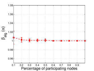
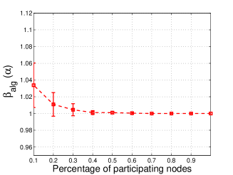
Figure 5: cDSMA accuracy for 10x10 nodes B-A graphs(left) and grids(right) as a function of the 1-median subgraph size: non-uniform service demand distribution ($s=1$).

TABLE II: Average normalized excess cost and hopcount for B-A and Grid networks: non uniform service demand (s=1)

	B-A graph				Grid network
Network size N	$\beta_{alg}(0.1)$	$h_{m}(0.1)$	$\beta_{alg}(0.4)$	$h_{m}(0.4)$	$\beta_{alg}(0.1)$	$h_{m}(0.1)$	$\beta_{alg}(0.4)$	$h_{m}(0.4)$
50(25x2)	1.0156$\pm$0.0205	1.60$\pm$0.48	1.0014$\pm$0.0038	1.85$\pm$0.35	1.0083$\pm$0.0068	1.50$\pm$0.37	1.0062$\pm$0.0047	1.10$\pm$0.22
100(25x4)	1.0070$\pm$0.0143	2.15$\pm$0.35	1.0015$\pm$0.0034	1.90$\pm$0.22	1.0553$\pm$0.0319	1.35$\pm$0.35	1.0025$\pm$0.0020	1.15$\pm$0.26
200 (40x5)	1.0016$\pm$0.0031	1.90$\pm$0.22	1.0003$\pm$0.0007	2.05$\pm$0.16	1.0510$\pm$0.0346	1.47$\pm$0.73	1.0031$\pm$0.0047	1.90$\pm$0.65
300 (60x5)	1.0029$\pm$0.0068	2.05$\pm$0.16	1.0000$\pm$0.0000	2.00$\pm$0.00

Figure 5 plots the average normalized excess cost for $s=1$. Again, the impact on the two types of synthetic graphs is different. For B-A graphs, the already high accuracy of cDSMA improves further. It lies within $1\%$ of the optimal already for $a=10\%$ and $N=100$ nodes and improves over the respective values under uniform service demand for all network sizes. Overall, the demand asymmetry magnifies the existing attraction forces towards the globally optimal service location, helping the algorithm to move away from locally optimal, yet globally suboptimal, hosts. The convergence speed of cDSMA is practically the same for networks in the range of 100 to 300 nodes.

On the other hand, the algorithm performance over grids is almost invariable with many entries in Tables I and II remaining practically the same. In fact, grid-like topologies set a negative benchmark for the performance of cDSMA requiring far more nodes within the 1-median subgraph to yield comparable accuracy with B-A graphs for the same network size and service demand distributions. Or, equivalently, for the same 1-median subgraph size, it needs a significantly higher asymmetry in the service demand distribution, as shown more clearly below.

VI-B2 Spatially correlated demand distribution

The service demand now exhibits spatial correlation. Interest in the service is concentrated in a particular graph neighborhood, as the case may be when the service has strongly local scope.

We model these scenarios by inserting a cluster of nodes with high service demand in a random area within a grid. The $K$ cluster nodes collectively represent some percentage $z\%$ of the total demand for the service, whereas the other $N-K$ nodes share the remaining $(100-z)\%$ of the demand. We call the ratio $z/(100-z)$ the demand spatial contrast $C_{sp}$. In 2D grids, clusters are formed by a cluster head node together with its four $1$-hop ($R=1$) or twelve $1$- and $2$-hop ($R=2$) neighbors. The contrast can then be written as:

$$C_{sp}(R,s)=\frac{\sum_{n=1}^{K}w(n;s,N)}{\sum_{n=K+1}^{N}w(n;s,N)}=\frac{\sum_{n=1}^{K}1/n^{s}}{\sum_{n=K+1}^{N}1/n^{s}}$$ (12)

and the average normalized excess cost becomes a function of both $\alpha$ and the contrast value.

The values of $\beta_{alg}(\alpha,C_{sp})$ under spatially random and correlated ($R=1$) distribution of demands are reported in Table III for a $10$x$10$ grid topology. Having the top demand values stemming from a certain network neighborhood we actually “produce” a single pole of strong attraction for the migrating service. Our algorithm now follows the demand gradient more effectively than before. As the percentage of the total demand held by the cluster nodes grows larger, resulting in higher spatial contrast, the pole gets even stronger driving the service firmly to the optimal location.

TABLE III: Average normalized excess cost under spatially correlated service demand

skewness $s$	$C_{sp}(1,s)$	$\beta_{alg}(0.1)$	$\beta_{alg}(0.1,C_{sp})$
1	0.786	1.035$\pm$0.027	1.016$\pm$0.023
2	8.540	1.003$\pm$0.006	1.0$\pm$0.0

It follows that $R=2$ and higher service demand distribution asymmetry $s$ only sharpen the spatial demand contrast, concentrating more the demand in space; namely, 61% of the service demand is spread across $13$ nodes for ($s=1,R=2$) and 89% across five nodes for ($s=2,R=1$). The attractive forces applied on the migrating service grow so that the algorithm finds easier its way towards the optimal location.

VI-C Experiments on real-world network topologies

Real-world networks do not typically have the predictable structure and properties of B-A graphs and grids and may differ substantially the one from another. Nevertheless, we show below that insightful analogies can be drawn between these networks and the B-A and grid topologies regarding the behavior of our service placement mechanism.

The ISP topology dataset includes 264 Tier-1, 244 Transit, and 342 stub ISP network topology files. They represent snapshots of 14 different ISP network topologies, as measured at different time epochs within the interval 2004-2008. We have focused on the larger Transit- and Tier-1 ISP datafiles, with topology sizes ranging from $100$ to $1000$ nodes, approximately. We chose to identify and primarily work with datasets, where the size of the maximal connected component, to be denoted by $mCC$, approaches the full vertex set of the measured graph . The connected components for each topology are retrieved via the well-known linear-time algorithm of Karp and Tarjan  [23]. Herein we present and discuss results from a representative subset of the datasets we experimented with, as shown in IV. They correspond to snapshots of four Tier-1 and three Transit ISP networks and were chosen so that there is adequate variance in size, diameter, and connectivity degree statistics.

TABLE IV: Selected ASes

Type	Dataset id	AS Number	Name	Extracted on
Tier-1	36	3549	Global Crossing	2006-05-03
	35	-//-	-//-	2006-07-13
	33	2914	NTTC-Gin	2008-12-03
	23	1239	Sprint	2008-09-30
	21	1239	-//-	2008-08-27
	27	3356	Level-3	2004-09-24
	13	-//-	-//-	2005-03-17
Transit	46	3292	TDC	2008-05-01
	41	680	DFN-IPX-Win	2006-05-03
	40	786	JanetUK	2008-07-01

Table V summarizes the performance of cDSMA over the real-world topologies. The listed results include the minimum number of nodes $|G^{i}|$ required to achieve a solution that lies within $2.5\%$ of the optimal and the average migration hop count $h_{m}$ for different levels of asymmetry in the service demand distribution.

The main observation is that both $\alpha_{0.025}$ and $|G^{i}|$ show a remarkable insensitivity to both topological structure and service demand dynamics. Although the considered ISP topologies differ significantly in size and diameter, the number of nodes we need to include in the $1$-median problem solution does not change. On the contrary, around half a dozen nodes suffices to get good accuracy even under uniform demand distribution, the least favorable scenario for our algorithm as discussed in Sections VI-A and VI-B. Likewise, $\alpha_{0.025}$ and $|G^{i}|$ remain practically invariable with the demand distribution skewness. Although for larger values of $s$, few nodes exhibit asymmetrically large demand values and become stronger attractors for the algorithm, the added value for the algorithm accuracy is negligible.

This two-way insensitivity of our algorithm bears two significant implications for its more practical implementation aspects. Firstly, the computational complexity when solving instances of the 1-median problem can be negligible and scales well with the size and diameter of the network. Secondly, the algorithm performance is robust to possibly inaccurate estimates of the service demand each node poses.

A last remark is appropriate with respect to the topological structure of these real-world topologies. The equally well algorithm behavior under uniform demand distribution ($s=0$) suggests that there is already adequate structure in the network topology. As the probability distribution of the connectivity degree in these networks suggests (see Fig. 6), there are high-degree nodes and considerable variance in the connectedness properties of nodes across the network. In fact, the high-degree nodes serve in a way similar to the high-degree nodes in B-A graphs; they are easily “identifiable” by our algorithm as low-cost hosts for the migrating service and, even for small 1-median subgraph sizes, their attraction forces are strong enough to pave a cost-effective service migration path.

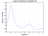
(a) dataset 36

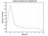
(b) dataset 35

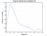
(c) dataset 33

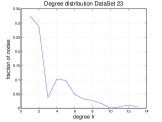
(d) dataset 23

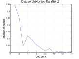
(e) dataset 21

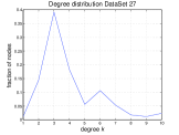
(f) dataset 27

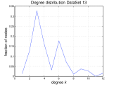
(g) dataset 13

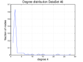
(h) dataset 46

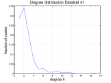
(i) dataset 41

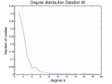
(j) dataset 40

Figure 6: Degree distributions of the ISP topology snapshots

TABLE V: Mean value of $\alpha_{\epsilon}$ for various datasets under different demand distributions

					s=0		s=1		s=2
Type	Dataset id	mCC nodes	Diameter	<Degree>	$\alpha_{0.025}$	$\lceil|G^{i}|\rceil$	$\alpha_{0.025}$	$\lceil|G^{i}|\rceil$	$\alpha_{0.025}$	$\lceil|G^{i}|\rceil$
Tier-1	36	76	10	3.71	0.047$\pm$0.001	4	0.047$\pm$0.002	4	0.046$\pm$0.001	4
	35	100	9	3.78	0.045$\pm$0.002	5	0.045$\pm$0.001	5	0.043$\pm$0.001	5
	33	180	11	3.53	0.024$\pm$0.002	5	0.022$\pm$0.002	4	0.019$\pm$0.002	4
	23	184	13	3.06	0.019$\pm$0.002	4	0.018$\pm$0.002	4	0.017$\pm$0.002	4
	21	216	12	3.07	0.016$\pm$0.002	4	0.016$\pm$0.002	4	0.014$\pm$0.003	4
	27	339	24	3.98	0.018$\pm$0.002	7	0.017$\pm$0.002	6	0.014$\pm$0.003	5
	13	378	25	4.49	0.012$\pm$0.002	5	0.012$\pm$0.002	5	0.011$\pm$0.002	5
Transit	46	71	9	3.30	0.033$\pm$0.003	3	0.027$\pm$0.004	2	0.026$\pm$0.003	2
	41	253	14	2.62	0.019$\pm$0.003	5	0.015$\pm$0.003	4	0.015$\pm$0.003	4
	40	336	14	2.69	0.012$\pm$0.003	5	0.012$\pm$0.002	5	0.013$\pm$0.002	5

VI-D cDSMA vs. locality-oriented service migration

The way cDSMA determines the service migration path clearly differentiates from typical “local-search” approaches. Local-search solutions such as the R-ball heuristic in [8], for example, restrict a-priori their search for a better service host to the neighborhood of the current service location. On the contrary, cDSMA focuses its search for the next service host in certain directions. Nodes lying across a (shortest) path, which serves many requests for a service, exhibit relatively high $wCBC$ values. The resulting 1-median subgraph is spatially stretched across that path and therefore oversteps the local neighborhood “barriers”.

To compare the above two approaches, we have implemented a Locality-Oriented Migration heuristic, hereafter abbreviated to LOM. In LOM we solve the 1-median problem within the direct neighborhood of $R$ hops around the current host and apply the same demand mapping mechanism (IV-C) to capture the demand load from nodes lying further than $R$ hops away from the current service host. The comparison of the two approaches for each ISP topology snapshot in Table VI proceeds as follows. We first generate asymmetric service demand (Zipf distribution with $s=1$) across the network. We compute the globally optimal service host node and we select a fixed set of service generation nodes, at $D_{gen}$ hops away from the optimal service location. We then calculate the values of $h_{m}$ and $\beta_{alg}$ metrics  for the two approaches, cDSMA and LOM. For cDSMA, we have set the parameter $\alpha=3\%$, meaning that the 1-median subgraph size ranges from 6 to 12 nodes for the networks listed in Table VI.

TABLE VI: convergence speed and accuracy comparison between LOM and cDSMA on realistic topologies

	Dataset 23				Dataset 33				Dataset 27				Dataset 13
$D_{gen}$	LOM		cDSMA		LOM		cDSMA		LOM		cDSMA		LOM		cDSMA
	$h_{m}$	$\beta_{alg}$	$h_{m}$	$\beta_{alg}(3\%)$	$h_{m}$	$\beta_{alg}$	$h_{m}$	$\beta_{alg}(3\%)$	$h_{m}$	$\beta_{alg}$	$h_{m}$	$\beta_{alg}(3\%)$	$h_{m}$	$\beta_{alg}$	$h_{m}$	$\beta_{alg}(3\%)$
3	1	1.1050	2	1	1	1.0308	2	1	1	1.1109	1	1.0057	1	1.1054	1	1
4	1	1.1275	3	1	1	1.3206	2	1	1	1.2523	1	1.0057	1	1.2312	1	1
5	1	1.1632	2	1	1	1.2800	1	1.2800	2	1.1109	1	1	1	1.0434	2	1
7	1	1.6060	2	1	3	1.0308	1	1.0308	3	1.1763	1	1	1	1.4202	1	1
10	–	–	–	–	–	–	–	–	1	1.7094	2	1	1	1.4604	2	1
13	–	–	–	–	–	–	–	–	2	1.8579	1	1.0057	3	1.6887	1	1.1054

Our expectation before the experiments was that the LOM heuristic would be characterized by overly higher number of migration hops since the latter is lower bounded by $D_{gen}/R$ when the service reaches the globally optimal location. Nevertheless, and interestingly enough, the LOM approach combines high excess costs with generally small number of migration hops, irrespective of the service generation location and for all topologies. Selecting “blindly” the $R$-hop neighbors of the current service host as future candidate hosts, LOM effectively introduces noise to the mechanism’s effort to detect the cost-effective service migration direction. With LOM the nodes in the 1-median subgraph are spread more unidirectionally around the service host and the demand mapping process projects more uniformly the demand contributions of the remaining nodes on them. Consequently, the migrating service gets easily trapped in some local minimum, which forces the migration process to stop too early to achieve an efficient solution. This resembles the behavior of the cDSMA in grids under uniform demand. There it was the topology of the network that induced a more local 1-median subgraph and attenuated the attraction force towards the optimal. With LOM, this locality is inherently imposed a-priori by the method, with similarly negative results.

On the other hand, the cDSMA heuristic seeks to choose the most “appropriate” candidate hosts, capable of leading the service fast to preferable/cost-minimizing locations, no matter what the shape/radius of the emerging $G^{i}$ neighborhood would be. Whereas, in a couple of cases that both approaches are trapped to a suboptimal place, e.g., Dataset 33 and $D_{gen}$=7, LOM needs three hops to get there, whereas cDSMA aborts after one hop.

This capability of cDSMA to make longer migration hops and accelerate its convergence to the (sub)optimal service location has another positive effect: the migration hop-count remains largely independent of the service generation host. This means that the mechanism does not favor nodes according to their proximity to the service demand and/or network topology hot spots, inducing a less dramatic yet welcome notion of fairness in the performance different network users get.

VII Related work

The problem of service placement has been predominantly treated as an instance of the broader family of (metric) facility location (FL) problems, which have found many different applications in areas as diverse as transportation networks and distributed computing. (Un)Capacitated FL problems is probably the most popular problem variant, where the objective is to minimize the combined cost of opening a facility and serving its clients and the number of facilities is not a priori bounded. The problem we address instead is an instance of k-median, $k=1$ in our case, problems, where no opening cost exists and the operational facilities cannot exceed $k$. Both problems are NP-hard for general topologies [5, 9]; thus, various approximations commonly requiring exact knowledge about their inputs, have been proposed to address them [11, 24].

The proposed approaches are typically categorized to centralized and distributed. The applicability of centralized solutions to large-scale data networks is severely undermined by the need for centralized decision-making and collection of global information about service demand and topology. In particular when this information varies dynamically, as with mobile networks, distributed solutions become mandatory and have recently received renewed attention [25].

One recently initiated research thread relates to the approximability of distributed approaches to the facility location problem. Moscibroda and Wattenhofer in [26] draw on a primal-dual approach earlier devised by Jain and Vazirani in [6], to derive a distributed algorithm that trades-off the approximation ratio with the communication overhead under the assumption of $O(logn)$ bits message size, where $n$ the number of clients. More recently, Pandit and Pemmaraju have derived an alterative distributed algorithm that compares favorably with the one in [26] in resolving the same trade-off [27].

Although the approximability studies can provide provable bounds for the run time and the obtainable quality of the solutions, they are typically outperformed by less mathematically rigorous yet practical heuristic solutions. Common to most of them is the service migration from the generator host towards its optimal location through a number of locally-determined hops that delineate a cost-decreasing path. What changes is the way decisions are made. Oikonomou et al.in  [7] exploit the shortest-path tree structures that are induced on the network graph by the routing protocol operation to estimate upper bounds for the aggregate cost in case service migrates at the 1-hop neighbors. Migration hops are therefore one physical hop long and this decelerates the migration process, especially in larger networks. Our algorithm resolves more efficiently the trade-off between convergence speed and accuracy; in fact, cDSMA maintains consistently high convergence speed over the real-world topologies while achieving very-close-to-optimal placements.

Even closer to our work is the upcoming paper of Smaragdakis et al. [8]. They reduce the original k-median problem in multiple smaller-scale 1-median problems solved within an area of r-hops from the current location of each service facility. Compared to cDSMA, the area over which they search for candidate next service hosts and upon which they map demand from the “outer” nodes is the r-hop neighbourhood of the current service location. In VI-D we have discussed in detail how cDSMA compares with a similar, local-search oriented approach.

Finally, cDSMA is an instance of a mechanism, where insights from Complex Network Theory help improve the performance of a network operation (here: service migration and optimal placement) significantly. Two more such examples have been reported in the area of Delay Tolerant Networks, where CNA has inspired the derivation of new routing protocols that, when correctly tuned, can improve performance significantly over more naive approaches [28, 29].

VIII Discussion-conclusions

Networked communication becomes more and more user-oriented. After the success of user-generated content, user-oriented service creation emerges as a new paradigm that will let individual users generate and make available services at minimum programming effort. Scalable distributed service migration mechanisms will be key to the successful proliferation of the paradigm.

We have mimicked earlier research work in treating the service placement problem in the general context of facility location problems. We have departed from it in exploiting complex network analysis for coming up with a scalable distributed service migration mechanism. We introduced a metric, weighted Conditional Betweeness Centrality ($wCBC$) that captures the topological centrality and demand aggregation capacity of individual nodes. The metric is used to select a small subset of significant nodes for solving the 1-median problem as well as easily map the demand of the remaining nodes on this subset. The service facilities migrate in the network towards the (sub)optimal location along a cost-decreasing path determined iteratively at the few intermediate service host nodes.

Both the network topology and spatial dynamics of service demand affect the accuracy and the convergence speed of the algorithm, giving rise to stronger/lighter attraction forces that drag the migrating service facilities towards the optimal location. In general, the higher the asymmetry in either of the two, the better the performance of the algorithm. The exhaustive evaluation of our algorithm on real-world topologies suggests that very good accuracy can be obtained when solving the 1-median problem with a very small number, in the order of ten, of nodes with the highest $wCBC$ scores. The result is insensitive to the network size and diameter and the asymmetry of demand distribution, hinting that real-world topologies have enough asymmetry to yield good performance of the algorithm. Moreover, the algorithm outperforms locality-oriented service migration and its accuracy and convergence speed are not dependent on the position of the service generation.

The proposed mechanism is highly decentralized; all nodes-candidates to host a service share the decision-making process for optimally placing the service in the network. It is also scalable in that it copes with the computational burden related to the solution of the $1$-median problem; this may become a difficult task for large-scale networks, especially when changes in the service demand characteristics call for its repeated execution. Nevertheless, topological and demand information still needs to propagate in the network. For small-size networks, topological information may become available through the operation of a link-state routing protocol that distributes and uses global topology information. For larger-scale networks, one way to acquire topology information would be through the deployment of some source-routing or path-switching protocol that carries information about the path it traverses on its headers. Information about the interest in services, on the other hand, may need more effort. Users increasingly subscribe to social networking sites and, sometimes consciously, give information about their interests and preferences. Profile-building mechanisms are components of peer-to-peer protocols as well; our mechanism will also be ultimately part of such a protocol.

Our problem formulation and the $wCBC$ metric we introduced for harnessing the computational burden of the $1$-median problem solution assume that the network exercises minimum hop count routing. Although minimum hop count routing is both simple and popular, network traffic engineering requires more elaborate routing solutions such as load-balancing/load adaptive routing [30]. We could generalize our treatment of the service migration problem to address these cases. First of all, the (conditional) betweenness centrality factor in the $wCBC$ metric definition is inherently flexible in that it considers shortest paths. Different routing metrics can be accommodated through changing the context of (shortest) path. For example, we could consider weighted graphs, where link weights may represent link capacities or propagation delays. A more substantial change in the metric would be to replace the shortest-path betweenness centrality with alternative $BC$ definitions: the random-walk betweeness centrality [31], which would resemble more a probabilistic, traffic demand oblivious routing implementation, or the k-betweenness centrality [32], which is closer to some short of multipath routing, even if it does not enforce independent, link/node disjoint paths. On the other hand, to accommodate other-than-min-hop-count routing in the content access leg, we would need a fundamental adaptation of the $1$-median problem formulation.

References

- [1] T. Plagemann, V. Goebel, A. Mauthe, L. Mathy, T. Turletti, and G. Urvoy-Keller, “From content distribution networks to content networks - issues and challenges,” Comput. Commun., vol. 29, no. 5, pp. 551–562, 2006.
- [2] V. Jacobson, D. Smetters, J. Thornton, M. Plass, N. Briggs, and R. Braynard, “Networking named content,” in 5th ACM CoNEXT 2009, Rome, Italy, December 2009, pp. 1–12.
- [3] A. Galis et al., “Management architecture and systems for future internet networks,” in FIA Book : "Towards the Future Internet - A European Research Perspective", Prague, May 2009, pp. 112–122.
- [4] E. Silva, L. F. Pires, and M. van Sinderen, “Supporting dynamic service composition at runtime based on end-user requirements,” in Proc. 1st International Workshop on User-generated Services (colocated with ICSOC2009), Stockholm, Sweden, November 2009.
- [5] P. Mirchandani and R.Francis, Discrete location theory, John Wiley and Sons, 1990.
- [6] K. Jain and V. V. Vazirani, “Approximation algorithms for metric facility location and k-median problems using the primal-dual schema and lagrangian relaxation,” Journal of ACM, vol. 48, no. 2, pp. 274–296, 2001.
- [7] K. Oikonomou and I. Stavrakakis, “Scalable service migration in autonomic network environments,” IEEE J.Sel. A. Commun., vol. 28, no. 1, pp. 84–94, 2010.
- [8] G. Smaragdakis, N. Laoutaris, K. Oikonomou, I. Stavrakakis, and A. Bestavros, “Distributed Server Migration for Scalable Internet Service Deployment,” IEEE/ACM Transactions on Networking, (To Appear) 2010.
- [9] O. Kariv and S. L. Hakimi, “An algorithmic approach to network location problems. ii: The p-medians,” SIAM Journal on Applied Mathematics, vol. 37, no. 3, pp. 539–560, 1979.
- [10] A. J. Goldman, “Optimal Center Location in Simple Networks,” Transportation Science, vol. 5, no. 2, pp. 212–221, 1971.
- [11] R. Solis-Oba, “Approximation algorithms for the k-median problem,” ser. Lecture Notes in Computer Science, vol. 3484. Springer, 2006, pp. 292–320.
- [12] L. C. Freeman, “A set of measures of centrality based on betweenness,” Sociometry, vol. 40, no. 1, pp. 35–41, 1977.
- [13] P. Pantazopoulos, I. Stavrakakis, A. Passarella, and M. Conti, “Efficient social-aware content placement for opportunistic networks,” in IFIP/IEEE WONS, Kranjska Gora, Slovenia, February, 3-5 2010.
- [14] T. H. Cormen, C. E. Leiserson, R. L. Rivest, and C. Stein, Introduction to Algorithms. The MIT Press, September 2001.
- [15] U. Brandes, “A faster algorithm for betweenness centrality,” Journal of Mathematical Sociology, vol. 25, pp. 163–177, 2001.
- [16] A. L. Barabasi and R. Albert, “Emergence of scaling in random networks,” Science, vol. 286, no. 5439, pp. 509–512, Oct 1999.
- [17] G. Siganos, M. Faloutsos, P. Faloutsos, and C. Faloutsos, “Power laws and the as-level internet topology,” IEEE/ACM Trans. Netw., vol. 11, no. 4, pp. 514–524, 2003.
- [18] J.-J. Pansiot, “mrinfo dataset.” [Online]. Available: http://svnet.u-strasbg.fr/mrinfo/
- [19] P. Mérindol, V. V. D. Schrieck, B. Donnet, O. Bonaventure, and J.-J. Pansiot, “Quantifying ASes multiconnectivity using multicast information,” in Proc. ACM USENIX Internet Measurement Conference (IMC), Chicago IL., February 2009.
- [20] J.-J. Pansiot, P. Mérindol, B. Donnet, and O. Bonaventure, “Extracting intra-domain topology from mrinfo probing,” in Proc. Passive and Active Measurement Conference (PAM), April 2010.
- [21] S. E. Deering, “Host extensions for ip multicasting,” RFC 1112 United States, 1989.
- [22] L. C. Freeman, “Centrality in social networks: Conceptual clarification,” Social Networks, vol. 1, pp. 215–239, 1979.
- [23] R. M. Karp and R. E. Tarjan, “Linear expected-time algorithms for connectivity problems (extended abstract),” in ACM STOC ’80, Los Angeles, California, 1980, pp. 368–377.
- [24] D. B. Shmoys, E. Tardos, and K. Aardal, “Approximation algorithms for facility location problems,” in 29th ACM STOC, 1997, pp. 265–274.
- [25] G. Wittenburg and J. Schiller, “A survey of current directions in service placement in mobile ad-hoc networks,” in IEEE PERCOM ’08, Hong Kong, March 17-21 2008, pp. 548–553.
- [26] T. Moscibroda and R. Wattenhofer, “Facility location: distributed approximation,” in PODC ’05, 2005, pp. 108–117.
- [27] S. Pandit and S. Pemmaraju, “Return of the primal-dual: distributed metric facilitylocation,” in ACM PODC ’09, 2009, pp. 180–189.
- [28] E. M. Daly and M. Haahr, “Social network analysis for routing in disconnected delay-tolerant manets,” in ACM MobiHoc ’07, Montreal, Quebec, Canada, 2007, pp. 32–40.
- [29] P. Hui, J. Crowcroft, and E. Yoneki, “Bubble rap: social-based forwarding in delay tolerant networks,” in ACM MobiHoc ’08, Hong Kong, Hong Kong, China, 2008, pp. 241–250.
- [30] B. Fortz, J. Rexford, and M. Thorup, “Traffic engineering with traditional ip routing protocols,” IEEE Communications Magazine, vol. 40, pp. 118–124, 2002.
- [31] M. J. Newman, “A measure of betweenness centrality based on random walks,” Social Networks, vol. 27, no. 1, pp. 39 – 54, 2005.
- [32] D. E. K. Jiang and D. Bader, “Generalizing k-betweenness centrality using short paths and a parallel multithreaded implementation,” in ICPP’09, Vienna, Austria, September 2009, pp. 542–549.