Direct Production of Lightest Regge Resonances

Abstract

We discuss direct production of Regge excitations in the collisions of massless four–dimensional superstring states, focusing on the first excited level of open strings ending on D–branes extending into higher dimensions. We construct covariant vertex operators and identify “universal” Regge states with the internal parts either trivial or determined by the world–sheet SCFT describing superstrings propagating on an arbitrary Calabi–Yau manifold. We evaluate the amplitudes involving one such massive state and up to three massless ones and express them in the helicity basis. The most important phenomenological applications of our results are in the context of low–mass string (and large extra dimensions) scenarios in which excited string states are expected to be produced at the LHC as soon as the string mass threshold is reached in the center–of–mass energies of the colliding partons. In order to facilitate the use of partonic cross sections, we evaluate them and tabulate for all production processes: gluon fusion, quark absorbing a gluon, quark–antiquark annihilation and quark-quark scattering.

I Introduction

The most direct way to exhibit the existence of fundamental strings is by discovering the effects of their vibrations. The particles that appear as the quanta of oscillating string modes are called Regge excitations and have squared masses quantized in the units of $M^{2}=1/\alpha^{\prime}$, where $\alpha^{\prime}$ is the Regge slope. Direct detection of such vibrating string modes is possible at the LHC, provided that $M$ is in the range of few TeVs. For a survey of low-mass superstring phenomenology and early references, see Refs. Antoniadis et al. (1998, 1998); Cullen et al. (2000); Burikham et al. (2005). At first, one would see Regge excitations indirectly, in the excess of photons Anchordoqui et al. (2008, 2008), jets Anchordoqui et al. (2008, 2009), heavy quarks Dong et al. (2010) and leptons due to the resonant enhancement of their production rates. As emphasized in Refs. Anchordoqui et al. (2008, 2008); Lüst et al. (2009, 2010), some of the most interesting signals of low-mass superstring theory are completely model-independent, i.e. they do not depend on the compactification space or on the SUSY breaking mechanism, hence by studying such processes we can avoid the landscape problem.

Once the mass threshold $M$ is crossed in the center–of–mass energies of the colliding partons, one would also see free Regge states produced directly, in association with jets, photons and other particles. In this paper, we discuss direct production of lightest Regge particles, i.e. the quanta of fundamental string harmonics with masses equal $M$.

The basic property of Regge states is that they populate linear trajectories, with the slope $\alpha^{\prime}$, correlating their masses and spins. At the $n$–th mass level,

$$M_{n}^{2}\ =\ n\ M^{2}\ \ \ ,\ \ \ n\in{\bf N}\ ,$$ (I.1)

the spins range from 0 to $n{+}1$. However, the spectrum of Regge excitations are highly model-dependent. For example, in the toroidal compactifications of a single ten-dimensional $D9$-brane one encounters 128 bosons and 128 fermions at the $n{=}1$ level. Most of these particles are tied to ${\cal N}{=}4$ supersymmetry of toroidal compactifications, however some of them are universal to all Calabi-Yau manifolds. No other Regge states than the universal ones can be observed as resonances in gluon-gluon scattering or in the processes involving only gluons and one pair of external fermions originating from D–brane intersections. In Ref. Anchordoqui et al. (2008), the spin content and multiplicities of the universal part of the first level have been disentangled by factorizing the four-point amplitudes. In this paper, we construct the covariant vertex operators creating universal particles. We include not only trivial internal parts but also the operators appearing in the world-sheet superconformal field theory (SCFT) of a superstring propagating on an arbitrary Calabi-Yau manifold (CYM). They create particles present in all compactifications preserving at least ${\cal N}{=}1$ SUSY and can decay into (or be created by the annihilation of) two gluons and/or gluinos. Furthermore, we construct the vertex operators for the lightest excited quarks, assuming that massless quarks originate from superstrings stretching between D-branes intersecting in the internal space.

With the vertex operators at hand, it is not too difficult to compute the scattering amplitudes involving one massive particle and two or three massless ones. The amplitudes relevant to the direct production of string resonances at the LHC are $p_{1}p_{2}\to p_{3}R$, where $p~{}(=g,q,\bar{q})$ are partons and $R$ is a massive string state.

The paper is organized as follows. In Section II we discuss some general factorization properties of string amplitudes. In Section III, we discuss the first massive level of open superstrings originating from a stack of $N$ D-branes extending into higher dimensions. Among the universal excitations of gauge bosons, we find one spin 2 particle, one vector and two complex scalars, with only spin 2 and a single scalar coupled to massless gauge bosons directly at the disk level. On the other hand, quarks exist in the excited spin 3/2 and 1/2 states. We construct the corresponding vertex operators. In Section IV, the wave functions describing massive particles with spins up to $J{=}2$ are written in the van der Waerden (helicity) representation. In Section V, we compute all amplitudes involving one of the universal Regge excitations and up to three massless partons. These amplitudes acquire a very simple form in the helicity basis, which also reveals certain selection rules similar (and related) to the vanishing of “all-plus” amplitudes at the zero mass level Stieberger and Taylor (2008). In Section VI, we square the appropriately crossed amplitudes for $p_{1}p_{2}\to p_{3}R$, average over initial helicities and colors and sum over the colors and spin directions of the outgoing particles. In order to facilitate phenomenological applications of the partonic cross sections, we tabulate squared amplitudes according to the production processes: gluon fusion, gluon-quark absorption, quark-antiquark annihilation and quark-quark scattering.

II Parton amplitudes and factorization on massive poles

The most direct way to see string effects is to measure the open string oscillator excitations, the so–called Regge modes. There are infinitely many open string Regge (SR) modes and their mass–squares are multiples of the string scale (I.1). To each level $n$ a set of states $|J,n\rangle$ belongs. The latter are classified by their spin $J$ with the highest possible spin $n+1$ limited by the oscillator number $n$. Each Standard Model (SM) particle is accompanied by an infinite number of these massive string excitations, i.e.  the latter carry SM quantum numbers and thus may be produced by $pp$–collisions.

SR excitations may appear in resonance channels of SM processes or may be directly produced as external states. While the first effect has been extensively studied in Cullen et al. (2000); Lüst et al. (2009, 2010) the latter effect will be discussed in this work. A first look at the couplings of massless SM particles to massive SR states is made by considering the factorization of higher–point amplitudes involving massless external states. In what follows we shall discuss this factorization on general grounds. We consider scattering amplitudes involving massless SM model open string fields $\Phi_{i}$ as external particles. These amplitudes are described by the exchange of the light (massless) SM fields and the tower of infinite many higher SR excitations.

Due to the extended nature of strings the string amplitudes are generically non–trivial functions of $\alpha^{\prime}$ in addition to the usual dependence on the kinematic invariants and degrees of freedom of the external states. In the effective field theory description this $\alpha^{\prime}$–dependence gives rise to a series of infinite many resonance channels due to Regge excitations and new contact interactions involving massless SM fields and massive SR states. As a consequence of unitarity an $N$–point tree–level string amplitude ${\cal M}(\Phi_{1},\ldots,\Phi_{N})$ can be written as an infinite sum over exchanges of (massive) intermediate string states $|J,n\rangle$ coupling to $N_{1}$ and $N_{2}$ external massless string states, with $N_{1}+N_{2}=N$. For each level this pole expansion gives rise to (new) $N_{1}+1$– and $N_{2}+1$–point couplings between the massive string states $|J,n\rangle$ and the $N_{1}$ and $N_{2}$ external massless string states, respectively.

In the following we illustrate this at the four–gluon amplitude, i.e. $\Phi_{i}=g_{i}$ and $N_{1}=N_{2}=2$. The latter gives rise to an infinite series of three–point couplings involving two massless gluons and massive string states $|J,n\rangle$. The general expression for the four–gluon amplitude in $D$ space–time dimensions is

$$\begin{array}[]{lcl}\displaystyle{{\cal M}(g_{1},g_{2},g_{3},g_{4})}&=&\displaystyle{2\ g_{YM}^{2}\ K_{4}(\varepsilon_{1},k_{1};\varepsilon_{2},k_{2};\varepsilon_{3},k_{3};\varepsilon_{4},k_{4})}\\[14.22636pt] &\times&\displaystyle{\left\{\ T^{a_{1}a_{2}a_{3}a_{4}}\ {\frac{B({\hat{s}},\hat{u})}{\hat{t}}}+T^{a_{2}a_{3}a_{1}a_{4}}\ {\frac{B(\hat{t},\hat{u})}{{\hat{s}}}}+T^{a_{3}a_{1}a_{2}a_{4}}\ {\frac{B({\hat{s}},\hat{t})}{\hat{u}}}\ \right\}\ ,}\end{array}$$ (II.3)

with the Euler Beta function

$$B(x,y)={\frac{\Gamma(x)\ \Gamma(y)}{\Gamma(x+y)}}\ ,$$ (II.4)

the kinematic factor Green and Schwarz (1982); Schwarz (1982)

$$\begin{array}[]{lcl}&&K_{4}(\varepsilon_{1},k_{1};\varepsilon_{2},k_{2};\varepsilon_{3},k_{3};\varepsilon_{4},k_{4})=\hat{t}\hat{u}\ (\varepsilon_{1}\varepsilon_{2})\ (\varepsilon_{3}\varepsilon_{4})+{\hat{s}}\hat{t}\ (\varepsilon_{1}\varepsilon_{4})\ (\varepsilon_{2}\varepsilon_{3})+{\hat{s}}\hat{u}\ (\varepsilon_{1}\varepsilon_{3})\ (\varepsilon_{2}\varepsilon_{4})\\ &&\hskip 12.80365pt+{\hat{s}}\ \left[\ (\varepsilon_{1}\varepsilon_{3})(\varepsilon_{2}k_{3})(\varepsilon_{4}k_{1})+(\varepsilon_{1}\varepsilon_{4})(\varepsilon_{2}k_{4})(\varepsilon_{3}k_{1})+(\varepsilon_{2}\varepsilon_{3})(\varepsilon_{1}k_{3})(\varepsilon_{4}k_{2})+(\varepsilon_{2}\varepsilon_{4})(\varepsilon_{1}k_{4})(\varepsilon_{3}k_{2})\ \right]\\ &&\hskip 12.80365pt+\hat{t}\ \left[\ (\varepsilon_{1}\varepsilon_{2})(\varepsilon_{3}k_{2})(\varepsilon_{4}k_{1})+(\varepsilon_{1}\varepsilon_{4})(\varepsilon_{2}k_{1})(\varepsilon_{3}k_{4})+(\varepsilon_{2}\varepsilon_{3})(\varepsilon_{1}k_{2})(\varepsilon_{4}k_{3})+(\varepsilon_{3}\varepsilon_{4})(\varepsilon_{1}k_{4})(\varepsilon_{2}k_{3})\ \right]\\ &&\hskip 12.80365pt+\hat{u}\ \left[\ (\varepsilon_{1}\varepsilon_{2})(\varepsilon_{3}k_{1})(\varepsilon_{4}k_{2})+(\varepsilon_{1}\varepsilon_{3})(\varepsilon_{2}k_{1})(\varepsilon_{4}k_{3})+(\varepsilon_{2}\varepsilon_{4})(\varepsilon_{1}k_{2})(\varepsilon_{3}k_{4})+(\varepsilon_{3}\varepsilon_{4})(\varepsilon_{1}k_{3})(\varepsilon_{2}k_{4})\ \right],\end{array}$$ (II.5)

and the color factor:

$$T^{a_{1}a_{2}a_{3}a_{4}}={\rm Tr}(T^{a_{1}}T^{a_{2}}T^{a_{3}}T^{a_{4}})+{\rm Tr}(T^{a_{4}}T^{a_{3}}T^{a_{2}}T^{a_{1}})\ .$$ (II.6)

Above, $\varepsilon_{i}$ are the polarization vectors and $k_{i}$ the external momenta of the four gluons. Furthermore, we have the kinematic invariants $\hat{s}=2\alpha^{\prime}k_{1}k_{2},\ \hat{t}=2\alpha^{\prime}k_{1}k_{3}$ and $\hat{u}=2\alpha^{\prime}k_{1}k_{4}$.

In what follows we shall concentrate on the partial amplitude ${\cal M}_{(1234)}$. According to the definition (II.2) we have: ${\cal M}_{(1234)}={\rm Tr}(T^{a_{1}}T^{a_{2}}T^{a_{3}}T^{a_{4}})\ A(1,2,3,4)$. With (c.f. Ref. Lüst et al. (2009))

$${\frac{B(\hat{s},\hat{u})}{\hat{t}}}={\frac{1}{\hat{t}\hat{u}}}\ {\frac{\Gamma(\hat{s})\ \Gamma(1+\hat{u})}{\Gamma(\hat{s}+\hat{u})}}=\sum_{n=0}^{\infty}\ \ {\frac{\gamma(n)}{\hat{s}+n}}\ ,$$ (II.7)

and

$$\gamma(n)={1\over n!}\ {\frac{\Gamma(\hat{u}+n)}{\Gamma(\hat{u}+1)}}={\frac{1}{n!}}\ {\frac{1}{\hat{u}}}\ \prod\limits_{j=1}^{n}(\hat{u}-1+j)$$ (II.8)

the amplitude (II.3) can be written as an infinite sum over $s$–channel poles at the masses (I.1) of the SR excitations:

$${\cal M}_{(1234)}(g_{1},g_{2},g_{3},g_{4})=2\ g_{YM}^{2}\ {\rm Tr}(T^{a_{1}}T^{a_{2}}T^{a_{3}}T^{a_{4}})\ K_{4}(\varepsilon_{1},k_{1};\varepsilon_{2},k_{2};\varepsilon_{3},k_{3};\varepsilon_{4},k_{4})\ \sum_{n=0}^{\infty}\ {\frac{\gamma(n)}{{\hat{s}}+n}}\ .$$ (II.9)

In (II.9) to each residue at ${\hat{s}}=-n$ a class of three–point couplings of two massless and one massive SR state $|J,n\rangle$ of a specific spin $J$ is associated, c.f. Fig. 1.

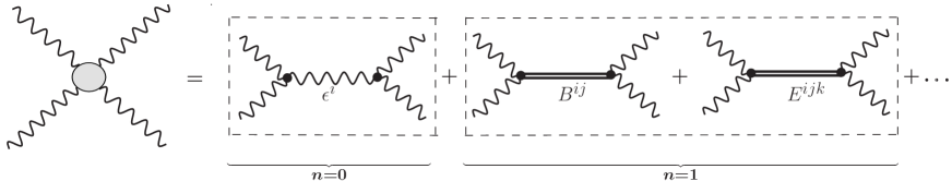
Figure 1: Factorization of four–gluon amplitude into pairs of two three–point couplings.

From (II.9) these three–point couplings are determined by the product $2\ g_{YM}^{2}\ \gamma(n)\ K_{4}$. To cast the residua of (II.9) into suitable form non–trivial factorization properties of the kinematic factor (LABEL:t8) have to hold.

We shall now evaluate for the amplitude (II.9) the contribution to the residue of the pole in ${\hat{s}}$ at ${\hat{s}}=-n$, with $n=0,1,\ldots$. At the level $n=0$ only a massless gluon with polarization $\varepsilon^{i}$ and spin $J=1$ is exchanged. Hence, we obtain the following residue at ${\hat{s}}=0$

$$\begin{array}[]{lcl}\displaystyle{{\rm Res}_{{\hat{s}}=0\atop\hat{u}=-\hat{t}}\ {\cal M}_{(1234)}(g_{1},g_{2},g_{3},g_{4})}&=&\displaystyle{2\ g_{YM}^{2}\ {\rm Tr}(T^{a_{1}}T^{a_{2}}T^{a_{3}}T^{a_{4}})}\\ &\times&\displaystyle{\gamma(0)\left.K_{4}(\varepsilon_{1},k_{1};\varepsilon_{2},k_{2};\varepsilon_{3},k_{3};\varepsilon_{4},k_{4})\right|_{{\hat{s}}=0\atop\hat{u}=-\hat{t}}}\\ &=&\displaystyle{\sum_{\varepsilon(k)}K_{3,0}(\varepsilon_{1},k_{1};\varepsilon_{2},k_{2};\varepsilon,k)\ K_{3,0}(\varepsilon_{3},k_{3};\varepsilon_{4},k_{4};\varepsilon,-k)\ ,}\end{array}$$ (II.10)

with the YM three–vertex:

$$\begin{array}[]{lcl}\displaystyle{K_{3,0}(\varepsilon_{1},k_{1};\varepsilon_{2},k_{2};\varepsilon_{3},k_{3})}&=&\displaystyle{g_{YM}\ {\rm Tr}(T^{a_{1}}[T^{a_{2}},T^{a_{3}}])}\\ &\times&\displaystyle{\left\{\ (\varepsilon_{1}\varepsilon_{2})\ (\varepsilon_{3}k_{1})+(\varepsilon_{1}\varepsilon_{3})\ (\varepsilon_{2}k_{3})+(\varepsilon_{2}\varepsilon_{3})\ (\varepsilon_{1}k_{2})\ \right\}\ .}\end{array}$$ (II.11)

Furthermore we have applied the completeness relations

$$\sum_{a}{\rm Tr}(T^{a_{1}}T^{a_{2}}T^{a})\ {\rm Tr}(T^{a}T^{a_{3}}T^{a_{4}})={\frac{1}{2}}\ {\rm Tr}(T^{a_{1}}T^{a_{2}}T^{a_{3}}T^{a_{4}})\ ,$$ (II.12)

with the sum over the Chan–Paton wavefunction of the intermediate state.

At the $n=1$ level exchanges of a spin $J=2$ state $B^{ij}$ and a $J=0$ state $E^{ijk}$ occur (c.f. Anchordoqui et al. (2008) for $D=4$). For the amplitude (II.9) we obtain the following residue at ${\hat{s}}=-1$

$$\begin{array}[]{lcl}\displaystyle{{\rm Res}_{{\hat{s}}=-1\atop\hat{u}=1-\hat{t}}\ {\cal M}_{(1234)}(g_{1},g_{2},g_{3},g_{4})}&=&\displaystyle{2\ g_{YM}^{2}\ {\rm Tr}(T^{a_{1}}T^{a_{2}}T^{a_{3}}T^{a_{4}})}\\ &\times&\displaystyle{\left.\gamma(1)\ K_{4}(\varepsilon_{1},k_{1};\varepsilon_{2},k_{2};\varepsilon_{3},k_{3};\varepsilon_{4},k_{4})\right|_{{\hat{s}}=-1\atop\hat{u}=1-\hat{t}}}\\ &=&\displaystyle{\sum_{E(k)}K_{3,1}(\varepsilon_{1},k_{1};\varepsilon_{2},k_{2};E,k)\ K_{3,1}(\varepsilon_{3},k_{3};\varepsilon_{4},k_{4};E,-k)}\\ &+&\displaystyle{\sum_{B(k)}K_{3,2}(\varepsilon_{1},k_{1};\varepsilon_{2},k_{2};B,k)\ K_{3,2}(\varepsilon_{3},k_{3};\varepsilon_{4},k_{4};B,-k)\ ,}\end{array}$$ (II.13)

with the two three–point vertices (in $D$ space–time dimensions)

$$\displaystyle{K_{3,1}(\varepsilon_{1},k_{1};\varepsilon_{2},k_{2};E,k)} = \displaystyle{6\ g_{YM}\ \left\{{\rm Tr}(T^{a_{1}}T^{a_{2}}T^{a_{3}})+{\rm Tr}(T^{a_{2}}T^{a_{1}}T^{a_{3}})\right\}\ E^{ijk}\ \varepsilon_{1i}\ \varepsilon_{2j}\ k_{1k}\ ,}$$ (II.14)

$$\displaystyle{K_{3,2}(\varepsilon_{1},k_{1};\varepsilon_{2},k_{2};B,k)} = \displaystyle{g_{YM}\ \left\{{\rm Tr}(T^{a_{1}}T^{a_{2}}T^{a_{3}})+{\rm Tr}(T^{a_{2}}T^{a_{1}}T^{a_{3}})\right\}}$$

$$\times \displaystyle{B^{ij}\ \left\{\ (k_{1}k_{2})\ \varepsilon_{1i}\varepsilon_{2j}-k_{1i}\varepsilon_{2j}\ (\varepsilon_{1}k_{2})-k_{2i}\varepsilon_{1j}\ (\varepsilon_{2}k_{1})+k_{1i}k_{2j}\ (\varepsilon_{1}\varepsilon_{2})\ \right\}\ ,}$$

involving two massless gluons and one massive string state $E^{ijk}$ and $B^{ij}$, respectively. In (II.13) the second equality follows by applying results from Yasuda (1988); Xiao and Zhu (2005, 2005).

III The first massive level

The first massive level of $D=10$ superstring, at the mass equal to the fundamental string scale $M$, consists of the quanta of fundamental harmonics. It is well known that it contains 128 bosonic degrees of freedom from the Neveu-Schwarz (NS) sector and 128 fermionic degrees of freedom from the Ramond (R) sector. These particles have the same Chan–Paton gauge charges as gauge bosons and gauginos because they all originate from open strings ending on D9-branes in $D=10$ spacetime. Hence it is appropriate to call them massive (or excited) “gluons” and “gluinos”. In addition, in specific models, there are similar particles associated to stacks of lower dimensional D-branes, with a reduced number of degrees of freedom. Furthermore, quarks, leptons and other MSSM fields arising from D-brane intersections, also appear in excited states at this level.

In Refs. Lüst et al. (2009, 2010) we stressed the universality (model–independence) of certain scattering amplitudes with an arbitrary number of external gluons and at most two fermions, at the leading disk order of string perturbations theory. This property allows testing the low string mass scenario at the LHC, in dijet mass distributions Anchordoqui et al. (2008) and other physical quantities Anchordoqui et al. (2009), in a completely model–independent manner, thus nullifying the notorious landscape problem. Our present goal is to identify the string excitations that can be produced on-shell, in parton collisions at center-of-mass energies above the string threshold mass $M$. Since the universal disk amplitudes do not depend on the extent of four-dimensional supersymmetry, it is clear that not all first level particles can be produced in such collisions. To some extent, this goal has been accomplished in Ref. Anchordoqui et al. (2008), where the relevant amplitudes have been factorized at the $s=M^{2}$ poles, exhibiting spin 2 and spin 0 resonances propagating in two-gluon channels etc. In this Section we go one step farther and identify the vertex operators of universal resonances. We will use them in the following Section to compute the amplitudes involving one massive and three massless states, which can be useful at the LHC for describing direct production of massive string states with large transverse momentum. Since we want to avoid discussing supersymmetry breaking already at this stage, we begin by truncating the first string level down to the universal ${\cal N}=1$ supermultiplets in $D=4$.

For maximally supersymmetric, toroidal compactifications of $D=10$ superstring, its excitations form supermultiplets of ${\cal N}=4$ supersymmetry. Before discussing the first excited level, we recall the vertices of massless particles, which arise from the zero modes and include, in the NS sector, the gluon $A$ and six real scalars $\phi^{j},~{}j=1,\dots,6.$ In the R sector, we have four gauginos $\lambda^{I},~{}I=1,\dots,4$. All in all, these zero mode form one ${\cal N}=4$ gauge supermultiplet. The NS sector vertices, in the $(-1)$-ghost picture, read:

$$V_{A^{a}}^{(-1)}(z,\epsilon,k) = g_{A}\ T^{a}\ e^{-\phi}\ \epsilon^{\mu}\,\psi_{\mu}\ e^{ikX}\ ,$$ (III.16)

$$V_{\phi^{a,j}}^{(-1)}(z,k) = g_{A}\ T^{a}\ e^{-\phi}\ \Psi^{j}\ e^{ikX}.$$ (III.17)

Here, $X,\psi,Z,\Psi$ are the fields of ${\cal N}=1$ worldsheet SCFT, with the Greek indices associated to $D=4$ spacetime fields $X^{\mu},\psi^{\nu}$ and the Latin lower case labeling internal $D=6$ (e.g. $Z^{i},\Psi^{j}$). $\phi$ is the scalar bosonizing the superghost system. For completeness, we write below the same vertices in the 0-ghost picture:

$$V_{A^{a}}^{(0)}(z,\epsilon,k) = \frac{g_{A}}{\sqrt{2\alpha^{\prime}}}\ T^{a}\ \epsilon^{\mu}\ [\ i\partial X_{\mu}+2\alpha^{\prime}\ k^{\nu}\psi_{\nu}\ \psi_{\mu}\ ]\ e^{ikX}\ ,$$ (III.18)

$$V_{\phi^{a,j}}^{(0)}(z,k) = \frac{g_{A}}{\sqrt{2\alpha^{\prime}}}\ T^{a}\ [\ i\partial Z^{j}+2\alpha^{\prime}\,k^{\nu}\psi_{\nu}\ \Psi^{j}\ ]\ e^{ikX}\ .$$ (III.19)

The R sector vertices, in the $(-1/2)$-ghost picture, read:

$$V_{\lambda^{a,I}}^{(-1/2)}(z,u,k) = g_{\lambda}\ T^{a}\ e^{-\phi/2}\ u^{\sigma}S_{\sigma}\ \Sigma^{I}\ e^{ikX}\ ,$$ (III.20)

$$V_{\bar{\lambda}^{a,I}}^{(-1/2)}(z,\bar{u},k) = g_{\lambda}\ T^{a}\ e^{-\phi/2}\ \bar{u}_{\dot{\sigma}}\bar{S}^{\dot{\sigma}}\ \overline{\Sigma}^{I}\ e^{ikX}.$$ (III.21)

Here, $S$ and $\bar{S}$ are the left and right-handed $SU(2)$ spin fields, respectively, while $\Sigma^{I}$ and $\overline{\Sigma}^{I}$ are the internal Ramond spin fields discussed in the following Subsection. The couplings are

$$g_{A}=(2\alpha^{\prime})^{1/2}\ g\quad,\quad g_{\lambda}=(2{\alpha^{\prime}})^{1/2}{\alpha^{\prime}}^{1/4}\ g\ ,$$ (III.22)

where $g$ is the gauge coupling. In the above definitions, $T^{a}$ are the Chan-Paton factors accounting for the gauge degrees of freedom of the two open string ends.

We will be also considering quarks and their first-level excitations. Assuming that the $SU(3)$ color group is associated to stack $a$, the vertices of quarks originating from strings attached at the other end to an intersecting stack $b$ are given by

$$V_{q^{\alpha}_{\beta}}^{(-1/2)}(z,u,k) = \sqrt{2}\ \alpha^{\prime 3/4}\,e^{\phi_{10}/2}\ \bigl{(}T^{\alpha}_{\beta}\bigr{)}^{\beta_{1}}_{\alpha_{1}}\ u^{\sigma}S_{\sigma}\ e^{-\phi/2}\ {\Xi}^{a\cap b}\ e^{ikX}\ ,$$

$$V_{\bar{q}^{\beta}_{\alpha}}^{(-1/2)}(z,\bar{u},k) = \sqrt{2}\ \alpha^{\prime 3/4}\ e^{\phi_{10}/2}\ \bigl{(}T^{\beta}_{\alpha}\bigr{)}^{\alpha_{1}}_{\beta_{1}}\ \bar{u}_{\dot{\sigma}}\bar{S}^{\dot{\sigma}}\ e^{-\phi/2}\ \bar{\Xi}^{a\cap b}\ e^{ikX}\ ,$$ (III.23)

where the Chan-Paton factors read

$$(T^{\alpha_{1}}_{\,\beta_{1}})_{\alpha_{2}}^{\beta_{2}}=\delta^{\alpha_{1}}_{\alpha_{2}}\delta^{\beta_{2}}_{\beta_{1}}$$ (III.24)

and $\Xi^{a\cap b}$ are the fermionic boundary changing operators. The latter carry the internal degrees of freedom of the Ramond sector associated to the internal part of the SCFT. Their two–point correlator is given by Lüst et al. (2009):

$$\langle\Xi^{a\cap b}(z_{1})\,\bar{\Xi}^{a\cap b}(z_{2})\rangle={\frac{1}{(z_{1}-z_{2})^{3/4}}}\ .$$ (III.25)

In general, such particles are in the bi-fundamental representations of the gauge groups associated to the two stacks. Note that the above vertices can be obtained from the gluino vertices (III.20) by simply adjusting the Chan-Paton factors and replacing the internal spin operators by the boundary changing operator. Thus up to such minor modifications, the vertices of excited quarks can be be “borrowed” from the R sector.

III.1 Bosons (NS sector)

For maximally supersymmetric, toroidal compactifications of $D=10$ superstring, NS and R sectors form one spin 2 ($J=2$) massive supermultiplet of ${\cal N}=4$ supersymmetry. The bosons form one symmetric tensor field $B_{mn}$ and one completely antisymmetric tensor field $E_{mnp}$. Here, the indices $(m,n,p)$ label $D=10$. All these particles are in the adjoint representation of the gauge group. The corresponding vertices, in the $(-1)$-ghost picture, read Koh et al. (1987):

$$V_{N\!S,a}^{(-1)}(z,k)=\frac{g_{A}}{\sqrt{2\alpha^{\prime}}}\ T^{a}\ e^{-\phi}(\,E_{mnp}\,\psi^{m}\psi^{n}\psi^{p}\,+\,B_{mn}\,i\partial X^{m}\psi^{n}\,+\,H_{m}\partial\psi^{m}\,)\,e^{ikX}\ ,$$ (III.26)

where $H_{m}$ is an auxiliary vector field. Note that at this level, the on-shell condition is $k^{2}=-\frac{1}{\alpha^{\prime}}$. The constraints due to the requirement of BRS invariance are:

$$~{}~{}~{}~{}k^{m}E_{mnp} = 0\ ,$$

$$2\alpha^{\prime}k^{m}B_{mn}+H_{n} = 0\ ,$$ (III.27)

$$B^{m}_{m}+k^{m}H_{m} = 0\ .$$

In $D=10$ all 128 bosonic degrees of freedom can be accounted for by setting $H=0$, i.e. with a traceless, transverse $B$ and transverse $E$. However, this auxiliary vector will be useful for discussing the spectrum of compactified theory.

In order to find out which of these particles can be produced in purely gluonic processes, we consider the disk amplitude involving one massive boson and an arbitrary number of gluons. Note that one of the gluon vertices must be in the $(-1)$-picture, see (III.16) while the rest in the 0-picture, see (III.18). Thus in (III.26), all world-sheet fermions must be associated to $D=4$ coordinates: $\psi^{m}=\psi^{\mu}$ etc. Furthermore, at the disk level, internal $\partial Z^{i}$ have no zero modes. We conclude that only $E_{\mu\nu\rho}$ and $B_{\mu\nu}$ interact with gluons at the disk level.

In $D=4$, a massive particle described by a transverse three-form is equivalent to a pseudoscalar with the wave function proportional to:

$$E_{\mu\nu\rho}\sim\epsilon_{\mu\nu\rho\lambda}\,k^{\lambda}.$$ (III.28)

A symmetric, transverse and traceless $B_{\mu\nu}$ gives rise to a spin 2 particle. However, this cannot be the end of the story. As pointed out in Ref. Anchordoqui et al. (2008), pseudoscalar resonances give rise to four-gluon scattering amplitudes with non-MHV helicity configurations, thus contradicting the fact that such amplitudes are zero at the disk level Stieberger and Taylor (2008). Thus we need another $J=0$ particle to cancel such pseudoscalar contributions. The relevant scalar is described by the following solution of the constraint (III.27):

$$E=0\qquad,\qquad B_{\mu\nu}=g_{\mu\nu}+2\alpha^{\prime}k_{\mu}k_{\nu}\qquad,\qquad H_{\mu}=2\alpha^{\prime}k_{\mu}\,.$$ (III.29)

As a result, we obtain one complex scalar $\Phi^{a}\equiv\Phi^{a+}$ ($\overline{\Phi}^{a}\equiv\Phi^{a-})$ and one $J=2$ particle $B^{a}$, with the vertices given by

$$V_{\Phi^{a\pm}}^{(-1)}(z,k) = \frac{g_{A}}{2\sqrt{2\alpha^{\prime}}}\,T^{a}\,e^{-\phi}\,\Bigl{[}\,(g_{\mu\nu}\,+\,2\alpha^{\prime}k_{\mu}k_{\nu})\,i\partial X^{\mu}\,\psi^{\nu}\ +\ 2\alpha^{\prime}k_{\mu}\partial\psi^{\mu}\Bigr{.}$$ (III.30)

$$\ \ \ \ \ \ \Bigl{.}\ \pm\ \frac{i}{6}\,2\alpha^{\prime}\,\epsilon_{\mu\nu\rho\lambda}\,k^{\lambda}\,\psi^{\mu}\,\psi^{\nu}\,\psi^{\rho}\,\Bigr{]}\,e^{ikX}\ ,$$

$$V_{B^{a}}^{(-1)}(z,\alpha,k) = \frac{g_{A}}{\sqrt{2\alpha^{\prime}}}\,T^{a}\,e^{-\phi}\,\alpha_{\mu\nu}\,i\partial X^{\mu}\psi^{\nu}\,e^{ikX},$$ (III.31)

The relative normalization of the scalar and pseudoscalar parts of the $J=0$ vertex will become clear later.

On the D–brane world–volume half of the space–time bulk SUSY is realized. The space–time SUSY currents contain the internal fields $\Sigma^{I},\overline{\Sigma}^{I}$ in the Ramond sector of the internal SCFT with the index $I$ specifying the SUSY. In type I or type IIB orientifolds D9–branes wrapped on a CYM yield ${\cal N}=1$ world–sheet SUSY. This SUSY gives rise to the pair $\Sigma,\overline{\Sigma}$ of internal fields whose operator product expansions (OPEs) are given by Banks et al. (1988)

$$\begin{array}[]{lcl}\Sigma(z)\ \overline{\Sigma}(w)&=&(z-w)^{-3/4}\ I+(z-w)^{1/4}\ {\frac{1}{2}}{\cal J}(w)+\ldots\ ,\\[5.69054pt] \Sigma(z)\ \Sigma(w)&=&(z-w)^{3/4}\ {\cal O}(w)+\ldots\ ,\end{array}$$ (III.32)

with the dimension one current ${\cal J}$ and dimension $3/2$ operator ${\cal O}$. These fields can be expressed in terms of a canonically normalized free scalar field $H$ as ${\cal J}=i\sqrt{3}\ \partial H$ and ${\cal O}=e^{i\sqrt{3}H}$, respectively. For the Ramond field $\Sigma$, which has charge $3/2$ under the current ${\cal J}$, we have $\Sigma=e^{i{\frac{\sqrt{3}}{2}}H}$. On the other hand, e.g. for D7–branes wrapped on 4–cycles we have ${\cal N}=2$ space–time SUSY on their world–volume while for space–time filling D3–branes ${\cal N}=4$ SUSY. These extended SUSY algebras give rise to the Ramond fields $\Sigma^{I},\overline{\Sigma}^{I}$ whose OPEs are given by Banks and Dixon (1988); Ferrara et al. (1989)

$$\begin{array}[]{lcl}\Sigma^{I}(z)\ \overline{\Sigma}^{J}(w)&=&(z-w)^{-3/4}\ \delta^{IJ}\ I+(z-w)^{1/4}\ {\cal J}^{IJ}(w)+\ldots\ ,\\[5.69054pt] \Sigma^{I}(z)\ \Sigma^{J}(w)&=&(z-w)^{-1/4}\ \psi^{IJ}(w)+(z-w)^{3/4}\ {\cal O}^{IJ}(w)+\ldots\ ,\end{array}$$ (III.33)

with the dimension one currents ${\cal J}^{IJ}$, the dimension $1/2$ operators $\psi^{IJ}$ and the dimension $3/2$ operators ${\cal O}^{IJ}$.

From the fact that $\Phi(J=0)$ and $B(J=2)$ resonances propagate in the universal amplitudes we can conclude that they must remain in the spectra of all self–consistent compactifications. In the context of SUSY, we can also ask whether these particles appear in two–gluino annihilations channels and in general, if there are other massive NS bosons that can be produced as a result of gluino scattering processes. These bosons are necessary to complete SUSY multiplets. In the ${\cal N}=1$ case, only one gluino species, say $\lambda^{1}\equiv\lambda$, remains in the spectrum, with a single internal Ramond field $\Sigma^{1}\equiv\Sigma$ in the vertex operator (III.20). If two gluinos are in the same helicity state, the internal charge conservation requires in the third (NS) vertex operator an internal field of charge $3$ under the current ${\cal J}$, therefore they cannot couple to $\Phi$ or $B$. In this case, they can couple to one complex scalar field $\Omega$ only, with the vertex operator

$$V_{\Omega^{a}}^{(-1)}(z,k)=g_{A}\ T^{a}\ e^{-\phi}\ {\cal O}\ e^{ikX}\ ,$$ (III.34)

with the charge $3$ field ${\cal O}$ appearing in the OPE (III.32). The field $\Omega$ is universal to all CY compactifications. Similarly, for extended space–time SUSY the fields ${\cal O}^{IJ}$ of the OPE (III.33) appear in the vertex operator (III.34). In the ${\cal N}=4$ case these fields ${\cal O}^{IJ}$ are essentially represented by products of three internal fermions $\Psi^{i}\Psi^{j}\Psi^{k}$.

On the other hand, if two gauginos carry opposite helicity, then the vertex operator of the third particle must contain an odd number (one or three) of worldsheet space–time fermions $\psi^{\mu}$ in order to get a non–vanishing correlator, c.f. Härtl et al. (2010). By using explicit forms of the underlying worldsheet correlators, it is easy to show that the coupling to scalar $\Phi$ vanishes on–shell, but there is a non–vanishing coupling to $B$. In addition, there is a non-vanishing coupling to a vector particle $W(J=1)$, universal to all ${\cal N}=1$ compactifications, with the vertex

$$V_{W^{a}}^{(-1)}(z,\xi,k)=g\ \sqrt{\frac{\alpha^{\prime}}{6}}\ T^{a}\ e^{-\phi}\ \xi_{\mu}\ \psi^{\mu}\ {\cal J}\ e^{ikX}\ ,$$ (III.35)

with $\cal J$ the dimension one worldsheet current appearing in the OPE (III.32). Similarly, for extended space–time SUSY the currents ${\cal J}^{IJ}$ of the OPE (III.33) appear in the vertex operator (III.35). Thus the universal part of the first massive level of the NS sector in ${\cal N}=1$ superstring compactifications consists of $B(J=2)$, $W(J=1)$, $\Phi(J=0)$ and $\Omega(J=0)$. Together with one massive spin 3/2 (Rarita-Schwinger) fermion from the R sector, $B(J=2)$ and $W(J=1)$ form one massive spin two supermultiplet Berkovits and Leite (1997). In addition, two complex scalars $\Phi(J=0)$ and $\Omega(J=0)$ combine with a spin 1/2 Dirac fermion to form one massive scalar supermultiplet.

III.2 Fermions (R sector)

Also for the fermions, we begin with the first massive level in $D=10$. In the R sector, the fermion vertex operator [in its canonical $(-1/2)$-ghost picture] is parametrized by two vectors, Majorana-Weyl spinors $v_{m}^{A}$ and $\bar{\rho}^{n}_{\dot{B}}$ of opposite chirality Koh et al. (1987):

$$V_{R,a}^{(-1/2)}(z,v,\bar{\rho},k)\ \ =\ \ C_{\Lambda}\ T^{a}\ \bigl{[}\,v_{m}^{A}\ i\partial X^{m}\ +\ 2\alpha^{\prime}\,\bar{\rho}^{m}_{\dot{B}}\ \psi_{m}\,\psi^{n}\,\Gamma_{n}^{\dot{B}A}\,\bigr{]}\,\Theta_{A}\ e^{-\phi/2}\ e^{ikX}\ .$$ (III.36)

Here, $A$ denotes a left-handed spinor index while $\dot{B}$ is its right handed counterpart. $\Gamma_{n}$ are $16\times 16$ Weyl blocks of the $D=10$ gamma matrices and $\Theta_{A}$ are the conformal weight $h=\frac{5}{8}$ chiral spin fields.

Requiring BRST invariance imposes two on-shell constraints on $v_{m}^{A}$ and $\bar{\rho}^{m}_{\dot{B}}$ which determine $\bar{\rho}$ in terms of $v$ and leave 144 independent components in the latter. Furthermore, a set of 16 spurious states exists which allows to take $\bar{\rho}$ and $v$ as transverse and $\Gamma$-traceless:

$$k^{m}\,v_{m}^{A}\ \ =\ \ v_{m}^{A}\,\Gamma^{m}_{A\dot{B}}\ \ =\ \ k_{m}\,\bar{\rho}^{m}_{\dot{B}}\ \ =\ \ \bar{\rho}^{m}_{\dot{B}}\,\Gamma_{m}^{\dot{B}A}\ \ =\ \ 0\ .$$ (III.37)

These $128=144-16$ physical degrees of freedom match the counting for bosons.

In $D=4$ compactifications, the spin field $\Theta$ breaks into the products of $SO(1,3)$ covariant spin fields $S_{\alpha},\bar{S}^{\dot{\beta}}$ times the internal spin fields of weight $h=\frac{3}{8}$. Our goal is to construct the vertex for the color triplets $Q$, the first excited level of quarks originating from brane intersections [created by vertex operators written in Eq. (III)]. To that end, we start from the $D=4$ decomposition of the vertex (III.36) and combine $h=\frac{5}{4}$ conformal fields of the spacetime SCFT (namely $\partial X^{\mu}S_{\alpha}$ and $\psi^{\mu}\psi^{\nu}S_{\alpha}$) with the $h=\frac{3}{8}$ fermionic boundary changing operator $\Xi^{a\cap b}$ which plays the role of internal spin field. Finally, we multiply by the $h=\frac{3}{8}$ superghost and the $h=-1$ exponential $e^{ikX}$ factors to obtain the desired $h=1$. In this way, we obtain:

$$\begin{array}[]{lcl}V_{Q^{\alpha}_{\beta}}^{(-1/2)}(z,v,\bar{\rho},k)&=&{\alpha^{\prime}}^{1/4}e^{\phi_{10}/2}\ \bigl{(}T^{\alpha}_{\beta}\bigr{)}^{\beta_{1}}_{\alpha_{1}}\ \bigl{[}\,iv_{\mu}^{\beta}\,\partial X^{\mu}-\sqrt{\alpha^{\prime}}\,\bar{\rho}^{\mu}_{\dot{\alpha}}\,\psi_{\mu}\,\psi^{\nu}\,\bar{\sigma}_{\nu}^{\dot{\alpha}\beta}\,\bigr{]}\,S_{\beta}\ e^{-\phi/2}\ \Xi^{a\cap b}\ e^{ikX}\ ,\\[2.84526pt] V_{\bar{Q}^{\beta}_{\alpha}}^{(-1/2)}(z,\bar{v},\rho,k)&=&{\alpha^{\prime}}^{1/4}e^{\phi_{10}/2}\ \bigl{(}T^{\beta}_{\alpha}\bigr{)}^{\alpha_{1}}_{\beta_{1}}\ \bigl{[}\,i\bar{v}^{\mu}_{\dot{\beta}}\,\partial X_{\mu}-\sqrt{\alpha^{\prime}}\,\rho_{\mu}^{\alpha}\,\psi^{\mu}\,\psi_{\nu}\,\sigma^{\nu}_{\alpha\dot{\beta}}\,\bigr{]}\,S^{\dot{\beta}}\ e^{-\phi/2}\ \bar{\Xi}^{a\cap b}\ e^{ikX}\ .\end{array}$$ (III.38)

The on-shell BRST constraints can be derived by following the analysis of Ref. Koh et al. (1987), although some numerical coefficients need adjustment from $D=10$ to $D=4$, due to gamma matrix contractions such as $\Gamma^{\mu\nu}\Gamma_{\nu}=-(D-1)\Gamma^{\mu}$. They are:

$$k_{\mu}\,\bar{v}^{\mu}_{\dot{\alpha}}\ \ =\ \ -\frac{3}{4\sqrt{\alpha^{\prime}}}\;\rho_{\mu}^{\beta}\,\sigma^{\mu}_{\beta\dot{\alpha}}\ ,\ \ \ \ \ \ \rho^{\alpha}_{\mu}\ \ =\ \sqrt{\alpha^{\prime}}\;\bar{v}_{\mu\dot{\beta}}\,\bar{\sigma}_{\nu}^{\dot{\beta}\alpha}\,k^{\nu}\ +\ \frac{1}{2}\;\rho_{\nu}^{\beta}\,(\sigma^{\nu}\,\bar{\sigma}_{\mu})_{\beta}\,\!^{\alpha}\ .$$ (III.39)

The above constraints allow expressing $\rho$ in terms of $\bar{v}$

$$\rho^{\mu\alpha}\ =\sqrt{\alpha^{\prime}}\;\bar{v}^{\mu}_{\dot{\beta}}\,\bar{\sigma}_{\nu}^{\dot{\beta}\alpha}\,k^{\nu}\ -\ \frac{2}{3}\sqrt{\alpha^{\prime}}\,k_{\nu}\,\bar{v}^{\nu}_{\dot{\beta}}\,\bar{\sigma}^{\mu\dot{\beta}\alpha},$$ (III.40)

with $\bar{v}$ subject to:

$$\bar{v}_{\dot{\alpha}}^{\mu}\,\bar{\sigma}_{\mu}^{\dot{\alpha}\beta}=2\alpha^{\prime}\,k_{\mu}\,\bar{v}^{\mu}_{\dot{\alpha}}\,\bar{\sigma}^{\dot{\alpha}\beta}_{\nu}\,k^{\nu}\ .$$ (III.41)

The latter impose 2 constraints on 8 (complex) parameters, leaving 6 wave functions describing spin 3/2 and spin 1/2 resonances $Q^{\star}(J=3/2)$ and $Q(J=1/2)$, respectively.

Next, we disentangle the different spin components of the solutions of Eq. (III.41). A general vector spinor of $SO(1,3)$ can be decomposed into irreducible representations of spin $3/2$ and $1/2$ according to $\bigl{(}\bf\frac{1}{2},\bf\frac{1}{2}\bigl{)}\otimes\bigl{(}\bf 0,\bf\frac{1}{2}\bigl{)}=\bigl{(}\bf\frac{1}{2},\bf 1\bigl{)}\oplus\bigl{(}\bf\frac{1}{2},\bf 0\bigl{)}$. The spin $3/2$ states $\bar{\chi}\in\bigl{(}\bf 1,\bf\frac{1}{2}\bigl{)}$ can be extracted by imposing the irreducibility conditions

$$\textrm{spin}\ \tfrac{3}{2}:\ \ \ \bar{v}^{\mu}_{\dot{\alpha}}(J=3/2)\ =\ \bar{\chi}^{\mu}_{\dot{\alpha}}\ \ \ \textrm{such that}\ \ \ \bar{\chi}^{\mu}_{\dot{\alpha}}\,\bar{\sigma}_{\mu}^{\dot{\alpha}\beta}\ \ =\ \ k_{\mu}\,\bar{\chi}^{\mu}_{\dot{\alpha}}\ \ =\ \ 0\ ,$$ (III.42)

which do indeed assemble 4 solutions of Eq. (III.41). In this case, the general formula (III.40) for $\rho$ simplifies since irreducibility kills the second term on the right hand side:

$$\textrm{spin}\ \tfrac{3}{2}:\ \ \ \rho^{\mu\alpha}(J=3/2)\ =\eta^{\mu\alpha}\ \ =\ \ \sqrt{\alpha^{\prime}}\;\bar{\chi}^{\mu}_{\dot{\beta}}\,\bar{\sigma}_{\nu}^{\dot{\beta}\alpha}\,k^{\nu}\ .$$ (III.43)

The latter can be recast as a massive Dirac equation for the four-spinor built from $\eta\oplus\bar{\chi}$:

$$\left(\begin{array}[]{cc}0&\not\!k_{\alpha\dot{\beta}}\\ \not\!k^{\dot{\alpha}\beta}&0\end{array}\right)\,\left(\begin{array}[]{c}\eta_{\mu\beta}\\ \,\bar{\chi}_{\mu}^{\dot{\beta}}\end{array}\right)\ \ =\ \ -\,m\left(\begin{array}[]{c}\eta_{\mu\alpha}\\ \,\bar{\chi}_{\mu}^{\dot{\alpha}}\end{array}\right)\ ,\ \ \ \ \ \ m\ \ =\ \ \frac{1}{\sqrt{\alpha^{\prime}}}\ .$$ (III.44)

The remaining 2 solutions of Eq. (III.41) describe a spin 1/2 particle and can be parametrized in terms of a left-handed Weyl spinor $\eta\in\bigl{(}\bf\frac{1}{2},\bf 0\bigl{)}$:

$$\bar{v}^{\mu}_{\dot{\beta}}=\eta^{\alpha}\sigma^{\nu}_{\alpha\dot{\beta}}\bigl{[}\delta^{\mu}_{\nu}+2\alpha^{\prime}k^{\mu}k_{\nu}\bigr{]}\ .$$ (III.45)

Incidentally, in $D=10$, similar solutions of the BRST conditions turned out to be spurious, but in any lower dimensions, they belong to the physical spectrum. This ties in with the observations made for real part of the massive scalar (III.31). Actually, the spin $1/2$ wave functions can be succinctly parametrized in terms of the right handed counterpart $\bar{\chi}_{\dot{\beta}}$ associated to $\eta$ via massive Dirac equation, $\bar{\chi}_{\dot{\beta}}=\sqrt{\alpha^{\prime}}\,\eta^{\alpha}\!\not\!k_{\alpha\dot{\beta}}$:

$$\textrm{spin}\ \tfrac{1}{2}:\ \ \ \bar{v}^{\mu}_{\dot{\alpha}}(J=1/2)\ \ =\ \ -\,\frac{\sqrt{\alpha^{\prime}}}{2\sqrt{2}}\;\bar{\chi}_{\dot{\beta}}\,(\bar{\sigma}^{\mu}\!\not\!k)^{\dot{\beta}}\,\!_{\dot{\alpha}}\ ,\ \ \ \ \ \ \rho_{\mu}^{\alpha}(J=1/2)\ \ =\ \ -\frac{1}{6\sqrt{2}}\;\bar{\chi}_{\dot{\beta}}\,\bar{\sigma}_{\mu}^{\dot{\beta}\alpha}.$$ (III.46)

Finally, we should mention that the vertex operators of excited gauginos can be obtained from the massive quarks (III.38) by adjusting normalization, Chan-Paton factors and the internal spin field:

$$\textrm{quarks:}\ \bigl{(}C_{Q},T^{\alpha}_{\beta},\Xi^{a\cap b}\bigr{)}\ \to\ \textrm{gluinos:}\ \bigl{(}C_{\Lambda},T^{a},\Sigma^{I}\bigr{)}\ .$$ (III.47)

These massive quarks (and gluinos) couple to their massless progenitors and gluons. In particular, $Q^{\star}(J=3/2)$ and $Q(J=1/2)$ propagate in the gluon-quark fusion channels of universal four-point amplitudes. Both spins present in the composite vertex for massive fermions belong to the spectrum regardless of the compactification geometry.

IV Weyl–van–der–Waerden formalism for wave functions of massless and massive particles

The vertex operators described in the previous Section depend on the wave functions of created string states. For our purposes, it is very convenient to use a unified “helicity notation”, i.e. the Weyl–van–der–Waerden formalism for both massless and massive particles. To that end, we use the notation of Wess and Bagger Wess and Bagger , with the metric signature $(-,+,+,+)$, however our conventions are slightly different than in the Refs. Lüst et al. (2009, 2010), therefore we phase them in gradually, in the context of wave functions describing massless particles.

IV.1 Massless spin 1/2 and 1 Wave Functions

Massless spin 1/2 fermions are usually described by two-component Weyl spinors, however anticipating the massive case, it is convenient to recall the four-component $\bigl{(}\bf\frac{1}{2},\bf\frac{1}{2}\bigl{)}$ representation of the wave functions $u_{\pm}(k)$ describing their $\pm\frac{1}{2}$ helicity eigenstates, respectively:

$$u_{+}(k) = |k\rangle=\binom{0}{k^{*\dot{a}}}\ ,$$

$$u_{-}(k) = |k]\,=\,\binom{k_{a}}{\,0\,}\,.$$ (IV.48)

The momentum $k$ is on-shell, $k^{2}=0$, and can be factorized as:

$$k_{\mu}\sigma_{a\dot{a}}^{\mu}=k_{a\dot{a}}=-k_{a}k_{\dot{a}}^{*}\ .$$ (IV.49)

Note that we are using $a$ and $\dot{a}$, as well as other letters from the beginning of the Latin alphabet, as $SU(2)\times SU(2)$ spinor indices that can be raised or lowered in the standard way by the $\epsilon$-symbol. The conjugate spinors are:

$$\bar{u}_{+}(k) = [k|=\,\left(k^{a},\,0\right)\ ,$$

$$\bar{u}_{-}(k) = \langle k|=\,\left(k_{\dot{a}}^{*},0\right)\ .$$ (IV.50)

Our conventions for the spinor products follow Ref. Dixon (1996):

$$\langle pq\rangle = \langle p|q\rangle=\bar{u}_{-}(p)u_{+}(q)~{}=~{}p_{\dot{a}}^{*}q^{*\dot{a}}\ ,$$

$${}[pq] = [p|q]\,=\bar{u}_{+}(p)u_{-}(q)~{}=~{}p^{a}q_{a}\ ,$$ (IV.51)

so that:

$$\langle pq\ \rangle[qp]=-2pq\ .$$ (IV.52)

The polarization vectors for a massless spin 1 particle with momentum $k$ utilize an arbitrary gauge-fixing “reference”momentum $r$ for each gauge boson Dixon (1996), which can be chosen to be any light-like momentum except $k$. They can be written as:

$$\epsilon_{\mu}^{+}(k,r) = ~{}\frac{\langle r|\gamma_{\mu}|k]}{\sqrt{2}\langle rk\rangle}~{}=~{}\frac{r_{\dot{a}}^{*}\bar{\sigma}_{\mu}^{\dot{a}a}k_{a}}{\sqrt{2}\langle rk\rangle}\ ,$$

$$\epsilon_{\mu}^{-}(k,r) = -\frac{[r|\gamma_{\mu}|k\rangle}{\sqrt{2}[rk]}=-\frac{r^{a}\sigma_{\mu a\dot{a}}k^{*\dot{a}}}{\sqrt{2}[rk]}\ .$$ (IV.53)

Of course, the physical amplitudes must not depend on the choice of reference momenta.

IV.2 Massive spin 1 and spin 2 bosons

A spin $J$ particle contains $2J+1$ spin degrees of freedom associated to the eigenstates of $J_{z}$. The choice of the quantization axis $z$ can be handled in an elegant way by decomposing the momentum $k$ into two arbitrary light-like reference momenta $p$ and $q$:

$$k^{\mu}=p^{\mu}+q^{\mu}\ ,\qquad k^{2}=-m^{2}=2pq\ ,\qquad p^{2}=q^{2}=0\ .$$ (IV.54)

Then the spin quantization axis is chosen as the direction of $p$ in the rest frame. The $2J+1$ spin wave functions depend of $p$ and $q$ Novaes and Spehler (1992); Spehler and Novaes (1991), however this dependence drops out in the amplitudes summed over all spin directions and in “unpolarized” cross sections.

The massive spin 1 wave functions $\xi^{\mu}$ are given by the following (transverse, i.e. $k_{\mu}\xi^{\mu}=0$) polarization vectors:

$$\xi^{\mu}(k,+1) = \frac{\sqrt{2}}{m}p_{\dot{a}}^{*}\bar{\sigma}^{\mu\dot{a}a}q_{a}\ ,$$

$$\xi^{\mu}(k,~{}0\,)~{} = \frac{1}{m}\bar{\sigma}^{\mu\dot{a}a}(p_{\dot{a}}^{*}p_{a}-q_{\dot{a}}^{*}q_{a})\ ,$$ (IV.55)

$$\xi^{\mu}(k,-1) = \frac{\sqrt{2}}{m}q_{\dot{a}}^{*}\bar{\sigma}^{\mu\dot{a}a}p_{a}\ .$$

The massive spin 2 wave functions are the traceless, symmetric tensors $\alpha^{\mu\nu}$ ($\alpha^{\mu\nu}=\alpha^{\nu\mu},~{}g_{\mu\nu}\alpha^{\mu\nu}=0$), subject to the transversality constraint $k_{\mu}\alpha^{\mu\nu}=0$. They can be written as Spehler and Novaes (1991):

$${\alpha}^{\mu\nu}(k,+2) = \frac{1}{2m^{2}}\bar{\sigma}^{\mu\dot{a}a}\bar{\sigma}^{\nu\dot{b}b}p_{\dot{a}}^{*}q_{a}p_{\dot{b}}^{*}q_{b}\ ,$$

$$\alpha^{\mu\nu}(k,+1) = \frac{1}{4m^{2}}\bar{\sigma}^{\mu\dot{a}a}\bar{\sigma}^{\nu\dot{b}b}\left[(p_{\dot{a}}^{*}p_{a}-q_{\dot{a}}^{*}q_{a})p_{\dot{b}}^{*}q_{b}+p_{\dot{a}}^{*}q_{a}(p_{\dot{b}}^{*}p_{b}-q_{\dot{b}}^{*}q_{b})\right]\ ,$$

$$\alpha^{\mu\nu}(k,~{}0~{}) = \frac{1}{2m^{2}\sqrt{6}}\bar{\sigma}^{\mu\dot{a}a}\bar{\sigma}^{\nu\dot{b}b}\left[(p_{\dot{a}}^{*}p_{a}-q_{\dot{a}}^{*}q_{a})(p_{\dot{b}}^{*}p_{b}-q_{\dot{b}}^{*}q_{b})-p_{\dot{a}}^{*}q_{a}q_{\dot{b}}^{*}p_{b}-q_{\dot{a}}^{*}p_{a}p_{\dot{b}}^{*}q_{b})\right]\ ,$$

$$\alpha^{\mu\nu}(k,-1) = \frac{1}{4m^{2}}\bar{\sigma}^{\mu\dot{a}a}\bar{\sigma}^{\nu\dot{b}b}\left[(q_{\dot{a}}^{*}q_{a}-p_{\dot{a}}^{*}p_{a})q_{\dot{b}}^{*}p_{b}+q_{\dot{a}}^{*}p_{a}(q_{\dot{a}}^{*}q_{a}-p_{\dot{b}}^{*}p_{b})\right]\ ,$$ (IV.56)

$$\alpha^{\mu\nu}(k,-2) = \frac{1}{2m^{2}}\bar{\sigma}^{\mu\dot{a}a}\bar{\sigma}^{\nu\dot{b}b}q_{\dot{a}}^{*}p_{a}q_{\dot{b}}^{*}p_{b}\ .$$

IV.3 Massive spin 1/2 and 3/2 fermions

Massive spin 1/2 wave functions are represented by four-component spinors

$$U(k)=\binom{\eta_{a}}{\bar{\chi}^{\dot{a}}}\ ,$$ (IV.57)

with the upper and lower components related by the Dirac equation

$$k_{\mu}\bar{\sigma}^{\mu\dot{a}a}\eta_{a}=-m\bar{\chi}^{\dot{a}}\qquad({\it i.e}.\\ k_{\mu}\sigma_{a\dot{a}}^{\mu}\bar{\chi}^{\dot{a}}=-m\eta_{a})\ .$$ (IV.58)

Their explicit form is:

$$U(k,+\frac{1}{2}) = \binom{\frac{\langle qp\rangle}{m}q_{a}}{p^{*\dot{a}}}\ ,$$

$$U(k,-\frac{1}{2}) = \binom{p_{a}}{\frac{[qp]}{m}q^{*\dot{a}}}\ .$$ (IV.59)

These wave functions should be substituted to Eqs. (III.46) and (III.38) in order to obtain the vertex for the $Q(J{=}1/2)$ resonance. Actually, Eq. (III.46) utilizes only the lower component $\bar{\chi}^{\dot{a}}$.

The wave functions of massive spin 3/2 particles are the vector spinors

$$R^{\mu}(k)=\binom{\eta_{a}^{\mu}}{\bar{\chi}^{\mu\dot{a}}}\ ,$$ (IV.60)

with the vectors constrained by

$$k_{\mu}\chi^{\mu\dot{a}}=k_{\mu}\eta^{\mu}_{a}=\sigma_{a\dot{a}}^{\mu}\bar{\chi}^{\mu\dot{a}}=\bar{\sigma}^{\mu\dot{a}a}\eta_{a}^{\mu}=0$$ (IV.61)

and satisfying the Dirac equation (IV.58). The wave functions describing individual spin configurations are Novaes and Spehler (1992):

$$R^{\mu}(k,+\frac{3}{2}) = \frac{1}{\sqrt{2}m}\binom{\frac{\langle qp\rangle}{m}q_{a}}{p^{*\dot{a}}}(p_{\dot{b}}^{*}\bar{\sigma}^{\mu\dot{b}b}q_{b})\ ,$$

$$R^{\mu}(k,+\frac{1}{2}) = \frac{\bar{\sigma}^{\mu\dot{b}b}}{\sqrt{6}m}\left[\binom{\frac{\langle qp\rangle}{m}q_{a}}{p^{*\dot{a}}}(p_{\dot{b}}^{*}p_{b}-q_{\dot{b}}^{*}q_{b})+\binom{\frac{\langle qp\rangle}{m}p_{a}}{-q^{*\dot{a}}}(p_{\dot{b}}^{*}q_{b})\right]\ ,$$

$$R^{\mu}(k,-\frac{1}{2}) = \frac{\bar{\sigma}^{\mu\dot{b}b}}{\sqrt{6}m}\left[\binom{p_{a}}{\frac{[qp]}{m}q^{*\dot{a}}}(p_{\dot{b}}^{*}p_{b}-q_{\dot{b}}^{*}q_{b})+\binom{-q_{a}}{\frac{[qp]}{m}p^{*\dot{a}}}(q_{\dot{b}}^{*}p_{b})\right]\ ,$$ (IV.62)

$$R^{\mu}(k,-\frac{3}{2}) = \frac{1}{\sqrt{2}m}\binom{p_{a}}{\frac{[qp]}{m}q^{*\dot{a}}}(q_{\dot{b}}^{*}\bar{\sigma}^{\mu\dot{b}b}p_{b})\ .$$

These wave functions should be substituted to Eqs. (III.42), (III.43) and (III.38) in order to obtain the vertex for the $Q^{\star}(J=3/2)$ resonance. Here again, only the lower component $\bar{\chi}^{\mu\dot{a}}$ enters into the vertex explicitly.

V Two– and three–particle decay amplitudes

With the vertices and wave functions at hand, we are ready to compute the amplitudes describing two– and three–particle decays of the bosons, $B(J=2)$, $W(J=1)$, $\Phi(J=0)$, $\Omega(J=0)$ and fermions $Q(J=1/2)$, $Q^{\star}(J=3/2)$. Although we are mainly interested in color octet bosons and fermion triplets, we will be considering bosons in the adjoint representation of a general $U(N)$ gauge group and fermions in its fundamental $N$ representation. Technical aspects of such computations have been discussed at length in Refs. Lüst et al. (2009) and Lüst et al. (2010), therefore we simply state the results, and go into more details only if the computations are complicated or they involve some new elements. Some amplitudes involving massive string states have been discussed before in Ref. Liu (1988).

Two-particle decays described by the amplitudes involving one massive state and two massless particles are particularly simple because the underlying SCFT correlators of three vertex operators inserted at the disk boundary do not depend on the vertex positions, therefore integrals over these positions are trivial. They are important, however, for the determination of proper normalization of vertex operators, which is done by factorizing a four-point scattering amplitude of massless particles at the resonance pole and comparing with appropriate products of three-point amplitudes. The vertex operators written in Section III have been already normalized in this way, so the amplitudes written below can serve as a check, as illustrated below in some more interesting cases.

We will be using the following shorthand notation for the amplitudes

$$R[J_{z};\lambda_{1},\lambda_{2},\dots]$$

denotes the amplitude for the decay of Regge state $R(=B,W,\dots)$ with the spin $z$-component $J_{z}$ into massless particles (quarks or gluons) labeled by $i=1,2,\dots$, with the momenta $k_{i}$, helicities $\lambda_{i}$ (they can be also specified by spinors or polarization vectors), etc. The massive particle will be labeled by the last index, i.e. $i=3$ in three-point functions and $i=4$ in four-point functions. The Mandelstam variables are defined as

$$s=-(k_{1}+k_{2})^{2}\ ,\qquad t=-(k_{1}+k_{3})^{2}\ ,\qquad u=-(k_{1}+k_{4})^{2}$$ (V.63)

with all momenta incoming and on-shell:

$$\sum_{i=1}^{4}k_{i}=0\ ,\qquad k_{1}^{2}=k_{2}^{2}=k_{3}^{2}=0\ ,\qquad k^{2}_{4}=-m^{2}=-\textstyle\frac{1}{\alpha^{\prime}}\ ,$$ (V.64)

which implies the following relation for the dimensionless variables:

$$\alpha^{\prime}s+\alpha^{\prime}t+\alpha^{\prime}u=1\ .$$ (V.65)

The spinor products will be abbreviated as

$$\langle k_{i}|k_{j}\rangle=\langle ij\rangle\ ,\qquad[k_{i}|k_{j}]=[ij]\ .$$ (V.66)

Finally, we recall the string formfactor

$$V_{t}=V(s,t,u)=\frac{\Gamma(1-\alpha^{\prime}s)\Gamma(1-\alpha^{\prime}u)}{\Gamma(1-\alpha^{\prime}s-\alpha^{\prime}u)}\ ,\qquad V_{s}=V_{t}(t\leftrightarrow s)\ ,\quad V_{u}=V_{t}(t\leftrightarrow u)\ .$$ (V.67)

Note that once the kinematic constraint (V.65) is implemented,

$$V_{t}=\frac{\Gamma(1-\alpha^{\prime}s)\Gamma(1-\alpha^{\prime}u)}{\Gamma(\alpha^{\prime}t)}\ ,$$ (V.68)

with the denominator $\Gamma(\alpha^{\prime}t)$ different from $\Gamma(1+\alpha^{\prime}t)$ that appears in the corresponding function describing the universal disk amplitudes with four massless particles Anchordoqui et al. (2008). CFT correlators involving various NS fermions and R spin fields are determined using the results of Härtl et al. (2010).

V.1 Massive spin 2 boson $B(J=2)$

We begin with the $B$-decays into gluons. The two-gluon channel is described by the amplitude

$$B[\alpha;\epsilon_{1},\epsilon_{2}]=(2\,d^{a_{1}a_{2}a_{3}})\ (4g\sqrt{2\alpha^{\prime}})\ \alpha_{\mu\nu}\left[\,(\epsilon_{2}k_{1})k_{2}^{\mu}\epsilon_{1}^{\nu}+(\epsilon_{1}k_{2})k_{1}^{\mu}\epsilon_{2}^{\nu}-(k_{1}k_{2})\epsilon_{2}^{\mu}\epsilon_{1}^{\nu}-(\epsilon_{1}\epsilon_{2})k_{1}^{\mu}k_{2}^{\nu}\,\right]\ .$$ (V.69)

In the prefactor, we singled out the color factor,

$$2\,d^{a_{1}a_{2}a_{3}}={\rm Tr}(T^{a_{1}}T^{a_{2}}T^{a_{3}})+{\rm Tr}(T^{a_{2}}T^{a_{1}}T^{a_{3}})\ ,$$ (V.70)

which appears after adding the contributions of the two orderings of the vertex operators inserted at the disk boundary. Note, that the form of the vertex (V.69) is reminiscent to the generic vertex (II). It is convenient to rewrite the amplitude (V.69) as

$$B[\alpha;\epsilon_{1},\epsilon_{2}]=4g\ (2\,d^{a_{1}a_{2}a_{3}})\ (2\alpha^{\prime})^{3/2}\ \mathscr{B}\left[\alpha;\epsilon_{1},\epsilon_{2}\right]$$ (V.71)

In order to rewrite the above amplitude in the helicity basis, for gluon helicity eigenstates, we substitute the wave functions (IV.53) and (IV.56). We find

$$\mathscr{B}[\alpha;\pm,\pm]=0\ ,$$ (V.72)

thus non-vanishing amplitudes must necessarily involve two gluons with opposite polarizations. They read:

$$\mathscr{B}\left[-2;+,-\right] = -\frac{1}{4}\langle p2\rangle^{2}[q1]^{2}\ ,$$

$$\mathscr{B}\left[-1;+,-\right] = -\frac{1}{2}\langle p2\rangle^{2}[q1][p1]\ ,$$

$$\mathscr{B}\left[~{}0~{};+,-\right] = -\frac{\sqrt{6}}{4}\langle p2\rangle^{2}[p1]^{2}\ ,$$ (V.73)

$$\mathscr{B}\left[+1;+,-\right] = +\frac{1}{2}\langle p2\rangle\langle q2\rangle[p1]^{2}\ ,$$

$$\mathscr{B}\left[+2;+,-\right] = -\frac{1}{4}\langle q2\rangle^{2}[p1]^{2}\ .$$

As a first check of the above result, we can examine the probability for the decay of unpolarized $B$ into a specific $(+,-)$ helicity configuration, by computing the sum

$$\sum_{\alpha=-2}^{+2}|B(\alpha;+,-)|^{2}=\frac{8}{\alpha^{\prime}}\,g^{2}(2\,d^{a_{1}a_{2}a_{3}})^{2}\ ,$$ (V.74)

which does indeed turn out to be independent of the choice of reference vectors $p$ and $q$. Now we can check if the result is consistent with string factorization. From Ref. Anchordoqui et al. (2008) we know that only the spin 2 resonance appears in the $s$-channel of the four-gluon amplitude ${\cal M}[g_{1}^{+},g_{2}^{-},g_{3}^{-},g_{4}^{+}]$, where it yields the following residue at $s=M^{2}=1/\alpha^{\prime}$

$${\rm Res}_{s=1/\alpha^{\prime}}\ {\cal M}[g_{1}^{+},g_{2}^{-},g_{3}^{-},g_{4}^{+}]\ \ =\ \ 4\,g^{2}{\rm Tr}(T^{a_{1}}T^{a_{2}}T^{a_{3}}T^{a_{4}})\,\alpha^{\prime}\langle 23\rangle^{2}[14]^{2}+\dots\ ,$$ (V.75)

where we picked up just one partial amplitude contribution. In order to compare our $B$-decay amplitude with the residue, we compute

$$\sum_{\alpha=-2}^{+2}B(\alpha;+,-)\ [B(\alpha;+,-)|_{(1\to 3,2\to 4)}]^{*}\ ,$$ (V.76)

with the color factor associated to the first ordering in Eq. (V.70), c.f. Eq. (II.12). The simplest way to perform the sum (V.76) is to set $p=k_{1}$ and $q=k_{2}$ because then only $J_{z}=-2$ contributes. Indeed, after combining the spin and color sums we recover Eq. (V.75), thus confirming the correct normalization of the vertex operator (III.31). Eqs. (V.71) and (V.73) can be also checked by comparing directly with Eq. (25) of Ref. Anchordoqui et al. (2008).

Three-gluon $B$–decays are described by the following amplitude

$$B [\alpha;\epsilon_{1},\epsilon_{2},\epsilon_{3}]~{}=~{}4\,g^{2}\sqrt{2\alpha^{\prime}}\ \big{(}\,V_{t}\,t^{a_{1}a_{2}a_{3}a_{4}}\ +\ V_{s}\,t^{a_{2}a_{3}a_{1}a_{4}}\ +\ V_{u}\,t^{a_{3}a_{1}a_{2}a_{4}}\,\big{)}$$

$$\times\,\biggl{\{}\,\frac{1}{s}\;\Bigl{[}\,(\epsilon_{2}\,\epsilon_{3})\,(\epsilon_{1}\,k_{2})\,(k_{3}^{\mu}\,\alpha_{\mu\nu}\,k_{3}^{\nu})\ -\ (\epsilon_{1}\,\epsilon_{3})\,(\epsilon_{2}\,k_{1})\,(k_{3}^{\mu}\,\alpha_{\mu\nu}\,k_{3}^{\nu})\ +\ (\epsilon_{1}\,\epsilon_{2})\,(\epsilon_{3}\,k_{2})\,(k_{1}^{\mu}\,\alpha_{\mu\nu}\,k_{3}^{\nu})\Bigr{.}\biggr{.}$$

$$\ \ \ \ \ \ \ \Bigl{.}-\ (\epsilon_{1}\,\epsilon_{2})\,(\epsilon_{3}\,k_{1})\,(k_{2}^{\mu}\,\alpha_{\mu\nu}\,k_{3}^{\nu})\ +\ (\epsilon_{1}\,k_{3})\,(\epsilon_{2}\,k_{1})\,(k_{3}^{\mu}\,\alpha_{\mu\nu}\,\epsilon_{3}^{\nu})\ -\ (\epsilon_{2}\,k_{3})\,(\epsilon_{1}\,k_{2})\,(k_{3}^{\mu}\,\alpha_{\mu\nu}\,\epsilon_{3}^{\nu})\Bigr{.}$$

$$\ \ \ \ \ \ \ \Bigl{.}+\ (\epsilon_{2}\,k_{1})\,(\epsilon_{3}\,k_{4})\,(k_{3}^{\mu}\,\alpha_{\mu\nu}\,\epsilon^{\nu}_{1})\ -\ (\epsilon_{1}\,k_{2})\,(\epsilon_{3}\,k_{4})\,(k_{3}^{\mu}\,\alpha_{\mu\nu}\,\epsilon^{\nu}_{2})\Bigr{.}$$

$$\ \ \ \ \ \ \ \Bigl{.}+\ \frac{1}{2\alpha^{\prime}}\;(\epsilon_{1}\,k_{2})\,(\epsilon^{\mu}_{2}\,\alpha_{\mu\nu}\,\epsilon^{\nu}_{3})\ -\ \frac{1}{2\alpha^{\prime}}\;(\epsilon_{2}\,k_{1})\,(\epsilon^{\mu}_{1}\,\alpha_{\mu\nu}\,\epsilon^{\nu}_{3})\Bigr{.}$$

$$\ \ \ \ \ \ \ \Bigl{.}-\ \frac{t}{2}\;(\epsilon_{1}\,\epsilon_{2})\,(k_{2}^{\mu}\,\alpha_{\mu\nu}\,\epsilon_{3}^{\nu})\ +\ \frac{u}{2}\;(\epsilon_{1}\,\epsilon_{2})\,(k_{1}^{\mu}\,\alpha_{\mu\nu}\,\epsilon_{3}^{\nu})\,\Bigr{]}$$

$$\ \ \ +\ \frac{1}{u}\;\Bigl{[}\,(\epsilon_{1}\,\epsilon_{3})\,(\epsilon_{2}\,k_{3})\,(k_{1}^{\mu}\,\alpha_{\mu\nu}\,k_{1}^{\nu})\ -\ (\epsilon_{1}\,\epsilon_{2})\,(\epsilon_{3}\,k_{2})\,(k_{1}^{\mu}\,\alpha_{\mu\nu}\,k_{1}^{\nu})\ +\ (\epsilon_{2}\,\epsilon_{3})\,(\epsilon_{1}\,k_{3})\,(k_{1}^{\mu}\,\alpha_{\mu\nu}\,k_{2}^{\nu})\Bigr{.}\biggr{.}$$

$$\ \ \ \ \ \ \ \Bigl{.}-\ (\epsilon_{2}\,\epsilon_{3})\,(\epsilon_{1}\,k_{2})\,(k_{1}^{\mu}\,\alpha_{\mu\nu}\,k_{3}^{\nu})\ +\ (\epsilon_{2}\,k_{1})\,(\epsilon_{3}\,k_{2})\,(k_{1}^{\mu}\,\alpha_{\mu\nu}\,\epsilon_{1}^{\nu})\ -\ (\epsilon_{3}\,k_{1})\,(\epsilon_{2}\,k_{3})\,(k_{1}^{\mu}\,\alpha_{\mu\nu}\,\epsilon_{1}^{\nu})\Bigr{.}$$

$$\ \ \ \ \ \ \ \Bigl{.}+\ (\epsilon_{3}\,k_{2})\,(\epsilon_{1}\,k_{4})\,(k_{1}^{\mu}\,\alpha_{\mu\nu}\,\epsilon^{\nu}_{2})\ -\ (\epsilon_{2}\,k_{3})\,(\epsilon_{1}\,k_{4})\,(k_{1}^{\mu}\,\alpha_{\mu\nu}\,\epsilon^{\nu}_{3})\Bigr{.}$$

$$\ \ \ \ \ \ \ \Bigl{.}+\ \frac{1}{2\alpha^{\prime}}\;(\epsilon_{2}\,k_{3})\,(\epsilon^{\mu}_{1}\,\alpha_{\mu\nu}\,\epsilon^{\nu}_{3})\ -\ \frac{1}{2\alpha^{\prime}}\;(\epsilon_{3}\,k_{2})\,(\epsilon^{\mu}_{1}\,\alpha_{\mu\nu}\,\epsilon^{\nu}_{2})\Bigr{.}$$

$$\ \ \ \ \ \ \ \Bigl{.}-\ \frac{s}{2}\;(\epsilon_{2}\,\epsilon_{3})\,(k_{3}^{\mu}\,\alpha_{\mu\nu}\,\epsilon_{1}^{\nu})\ +\ \frac{t}{2}\;(\epsilon_{2}\,\epsilon_{3})\,(k_{2}^{\mu}\,\alpha_{\mu\nu}\,\epsilon_{1}^{\nu})\,\Bigr{]}$$

$$\ \ \ +\ \frac{1}{t}\;\Bigl{[}\,(\epsilon_{1}\,\epsilon_{2})\,(\epsilon_{3}\,k_{1})\,(k_{2}^{\mu}\,\alpha_{\mu\nu}\,k_{2}^{\nu})\ -\ (\epsilon_{2}\,\epsilon_{3})\,(\epsilon_{1}\,k_{3})\,(k_{2}^{\mu}\,\alpha_{\mu\nu}\,k_{2}^{\nu})\ +\ (\epsilon_{1}\,\epsilon_{3})\,(\epsilon_{2}\,k_{1})\,(k_{2}^{\mu}\,\alpha_{\mu\nu}\,k_{3}^{\nu})\Bigr{.}\biggr{.}$$

$$\ \ \ \ \ \ \ \Bigl{.}-\ (\epsilon_{1}\,\epsilon_{3})\,(\epsilon_{2}\,k_{3})\,(k_{1}^{\mu}\,\alpha_{\mu\nu}\,k_{2}^{\nu})\ +\ (\epsilon_{3}\,k_{2})\,(\epsilon_{1}\,k_{3})\,(k_{2}^{\mu}\,\alpha_{\mu\nu}\,\epsilon_{2}^{\nu})\ -\ (\epsilon_{1}\,k_{2})\,(\epsilon_{3}\,k_{1})\,(k_{2}^{\mu}\,\alpha_{\mu\nu}\,\epsilon_{2}^{\nu})\Bigr{.}$$

$$\ \ \ \ \ \ \ \Bigl{.}+\ (\epsilon_{1}\,k_{3})\,(\epsilon_{2}\,k_{4})\,(k_{2}^{\mu}\,\alpha_{\mu\nu}\,\epsilon^{\nu}_{3})\ -\ (\epsilon_{3}\,k_{1})\,(\epsilon_{2}\,k_{4})\,(k_{2}^{\mu}\,\alpha_{\mu\nu}\,\epsilon^{\nu}_{1})\Bigr{.}$$

$$\ \ \ \ \ \ \ \Bigl{.}+\ \frac{1}{2\alpha^{\prime}}\;(\epsilon_{3}\,k_{1})\,(\epsilon^{\mu}_{1}\,\alpha_{\mu\nu}\,\epsilon^{\nu}_{2})\ -\ \frac{1}{2\alpha^{\prime}}\;(\epsilon_{1}\,k_{3})\,(\epsilon^{\mu}_{2}\,\alpha_{\mu\nu}\,\epsilon^{\nu}_{3})\Bigr{.}$$

$$\ \ \ \ \ \ \ \Bigl{.}-\ \frac{u}{2}\;(\epsilon_{1}\,\epsilon_{3})\,(k_{1}^{\mu}\,\alpha_{\mu\nu}\,\epsilon_{2}^{\nu})\ +\ \frac{s}{2}\;(\epsilon_{1}\,\epsilon_{3})\,(k_{3}^{\mu}\,\alpha_{\mu\nu}\,\epsilon_{2}^{\nu})\,\Bigr{]}$$

$$\ \ \ \biggl{.}\ -\ \frac{1}{2}\;\Bigl{[}\,(\epsilon_{1}\,\epsilon_{2})\,\epsilon_{3}^{\mu}\,\alpha_{\mu\nu}\,(k_{2}^{\nu}-k_{1}^{\nu})\ +\ (\epsilon_{2}\,\epsilon_{3})\,\epsilon_{1}^{\mu}\,\alpha_{\mu\nu}\,(k_{3}^{\nu}-k_{2}^{\nu})\ +\ (\epsilon_{1}\,\epsilon_{3})\,\epsilon_{2}^{\mu}\,\alpha_{\mu\nu}\,(k_{1}^{\nu}-k_{3}^{\nu})\,\Bigr{]}\biggr{\}}\ ,$$ (V.77)

with the color factor

$$t^{a_{1}a_{2}a_{3}a_{4}} = {\rm Tr}(T^{a_{1}}T^{a_{2}}T^{a_{3}}T^{a_{4}})-{\rm Tr}(T^{a_{4}}T^{a_{3}}T^{a_{2}}T^{a_{1}})$$ (V.78)

$$= i\,(d^{a_{1}a_{4}n}f^{a_{2}a_{3}n}-d^{a_{2}a_{3}n}f^{a_{1}a_{4}n})\ ,$$

i.e. $t^{a_{1}a_{2}a_{3}a_{4}}={\rm Tr}(T^{a_{1}}T^{a_{2}}T^{a_{3}}T^{a_{4}})-{\rm Tr}(T^{a_{1}}T^{a_{4}}T^{a_{3}}T^{a_{2}})$, $t^{a_{2}a_{3}a_{1}a_{4}}={\rm Tr}(T^{a_{1}}T^{a_{4}}T^{a_{2}}T^{a_{3}})-{\rm Tr}(T^{a_{1}}T^{a_{3}}T^{a_{2}}T^{a_{4}})$ and $t^{a_{3}a_{1}a_{2}a_{4}}={\rm Tr}(T^{a_{1}}T^{a_{2}}T^{a_{4}}T^{a_{3}})-{\rm Tr}(T^{a_{1}}T^{a_{3}}T^{a_{4}}T^{a_{2}})$. Note that the massless (II.3) and massive (V.77) amplitudes have different group structures, c.f. Eq.(V.78) and (II.6), respectively. This is explained in the following.

Generally, under world–sheet parity an $N$–point open superstring amplitude $A(1,\ldots,N)$ behaves as

$$A(1,\ldots,N)=\left(\prod_{i=1}^{N}(-1)^{\alpha^{\prime}m_{i}^{2}+\varepsilon}\right)\ A(N,\ldots,1)\ ,$$ (V.79)

with $m_{i}^{2}$ the masses of the external open string states. Furthermore, for $SO(N)$ representations we have $\varepsilon=1$ and $\varepsilon=0$ for $USp(N)$ representations Green et al. ; Angelantonj and Sagnotti (2002). Further relations between subamplitudes are obtained by analyzing their monodromy behavior w.r.t. to contour integrals in the complex plane Stieberger (2009). As a consequence for amplitudes involving only massless external string states ($m_{i}^{2}=0$) the full set of relations allows to reduce the number of independent subamplitudes to $(N-3)!$ Stieberger (2009); Bjerrum-Bohr et al. (2009). However, the set of relations for the massless case does not hold in the case if $m_{i}^{2}\neq 0$ and new monodromy relations have to be derived.

For the case at hand, i.e. $m_{i}=0,\ i=1,2,3$ and $m_{4}^{2}=\alpha^{\prime-1}$, the partial amplitudes are odd under the parity transformation. Hence from (V.79) we deduce:

$$\begin{array}[]{lcl}A(1,2,3,4)&=&-A(1,4,3,2)\ ,\\ A(1,2,4,3)&=&-A(1,3,4,2)\ ,\\ A(1,3,2,4)&=&-A(1,4,2,3)\ .\end{array}$$ (V.80)

This fact is manifest in the full amplitude (V.77) due to the color factor (V.78). After applying the contour arguments of Stieberger (2009) the following monodromy relation can be established for the case at hand:

$$A(1,2,3,4)-e^{i\pi\alpha^{\prime}s}\ A(1,2,4,3)-e^{-i\pi\alpha^{\prime}u}\ A(1,4,2,3)=0\ .$$ (V.81)

Together with (V.80) this relation allows to express all six partial amplitudes in terms of one, say $A(1,2,3,4)$:

$$\begin{array}[]{lcl}\displaystyle{A(1,4,3,2)}&=&\displaystyle{-A(1,2,3,4)\ ,}\\[14.22636pt] \displaystyle{A(1,2,4,3)}&=&\displaystyle{-A(1,3,4,2)={\frac{\sin(\pi\alpha^{\prime}u)}{\sin(\pi\alpha^{\prime}t)}}\ A(1,2,3,4)\ ,}\\[14.22636pt] \displaystyle{A(1,3,2,4)}&=&\displaystyle{-A(1,4,2,3)=-{\frac{\sin(\pi\alpha^{\prime}s)}{\sin(\pi\alpha^{\prime}t)}}\ A(1,2,3,4)\ .}\end{array}$$ (V.82)

Note, that (V.81) differs from the monodromy relation for the massless case, c.f. Eq. (4.8) of Stieberger (2009). As a consequence also the solution (V.82) is different than in the massless case, c.f. Eq. (4.10) of Stieberger (2009). It is easy to see that the relations (V.82) are indeed satisfied by the result (V.77).

In order to represent the amplitude (V.77) in the helicity basis, we rewrite it as:

$$B[\alpha;\epsilon_{1},\epsilon_{2},\epsilon_{3}]~{}=~{}8\,g^{2}\big{(}\,V_{t}\,t^{a_{1}a_{2}a_{3}a_{4}}+V_{s}\,t^{a_{2}a_{3}a_{1}a_{4}}+V_{u}\,t^{a_{3}a_{1}a_{2}a_{4}}\,\big{)}\ \sqrt{2\alpha^{\prime}}\ \mathscr{B}[\alpha;\epsilon_{1},\epsilon_{2},\epsilon_{3}]\ .$$ (V.83)

We find

$$\mathscr{B}[\alpha;\pm,\pm,\pm]=0\ ,$$ (V.84)

therefore non-vanishing amplitudes always involve one gluon of a given helicity and two of the opposite one. They have a very simple form:

$$\mathscr{B}\left[-2;+,+,-\right] ~{}=~{}\frac{1}{2\sqrt{2}}\ \!\frac{\langle p3\rangle^{4}}{\langle 12\rangle\langle 23\rangle\langle 31\rangle}\ ,$$

$$\mathscr{B}\left[-1;+,+,-\right] ~{}=~{}\frac{1}{\sqrt{2}}\ \,\frac{\langle p3\rangle^{3}\langle 3q\rangle}{\langle 12\rangle\langle 23\rangle\langle 31\rangle}\ ,$$

$$\mathscr{B}\left[~{}0~{};+,+,-\right] ~{}=~{}\frac{\sqrt{3}}{2}\ \,\frac{\langle p3\rangle^{2}\langle 3q\rangle^{2}}{\langle 12\rangle\langle 23\rangle\langle 31\rangle}\ ,$$ (V.85)

$$\mathscr{B}\left[+1;+,+,-\right] ~{}=~{}\frac{1}{\sqrt{2}}\ \,\frac{\langle q3\rangle^{3}\langle 3p\rangle}{\langle 12\rangle\langle 23\rangle\langle 31\rangle}\ ,$$

$$\mathscr{B}\left[+2;+,+,-\right] ~{}=~{}\frac{1}{2\sqrt{2}}\ \!\frac{\langle q3\rangle^{4}}{\langle 12\rangle\langle 23\rangle\langle 31\rangle}\ .$$

Similarly to the two-gluon case, we can consider the case of unpolarized $B$ decaying into a specific helicity configuration of the three gluons. By using Eqs. (V.83) and (V.85), we obtain

$$\sum_{\alpha=-2}^{+2}|B(\alpha;+,+,-)|^{2}=16\,g^{4}\,\frac{(1-\alpha^{\prime}s)^{4}}{\alpha^{\prime 3}\,s\,t\,u}\,|V_{t}\,t^{a_{1}a_{2}a_{3}a_{4}}+V_{s}\,t^{a_{2}a_{3}a_{1}a_{4}}+V_{u}\,t^{a_{3}a_{1}a_{2}a_{4}}|^{2}\ .$$ (V.86)

Next, we turn to $B$-decays into fermions. The quark-antiquark channel is described by the amplitude

$$B[\alpha;u_{1},\bar{u}_{2}]=(T^{a})^{\alpha_{1}}_{\alpha_{2}}(g\sqrt{2\alpha^{\prime}})\,k_{1}^{\mu}\alpha_{\mu\nu}\,u_{1}^{\lambda}\sigma^{\nu}_{\lambda\dot{\rho}}\bar{u}^{\dot{\rho}}_{2}\ ,$$ (V.87)

which we rewrite as:

$$B[\alpha;u_{1},\bar{u}_{2}]=g\,(T^{a})^{\alpha_{1}}_{\alpha_{2}}\ (2\alpha^{\prime})^{3/2}\mathscr{B}\left[\alpha;u_{1},\bar{u}_{2}\right]\ .$$ (V.88)

For the specific $({+}{\textstyle\frac{1}{2}},{-}{\textstyle\frac{1}{2}})$ helicity configuration of the antiquark-quark pair, we obtain:

$$\mathscr{B}\left[-2;{+}{\textstyle\frac{1}{2}},{-}{\textstyle\frac{1}{2}}\right] = \frac{1}{2}\ \langle p1\rangle\langle p2\rangle[q1]^{2}\ ,$$

$$\mathscr{B}\left[-1;{+}{\textstyle\frac{1}{2}},{-}{\textstyle\frac{1}{2}}\right] = \frac{1}{4}\ \langle p2\rangle[q1]\,\big{(}\langle q1\rangle[1q]-3\langle p1\rangle[1p]\big{)}\ ,$$

$$\mathscr{B}\left[~{}0~{};{+}{\textstyle\frac{1}{2}},{-}{\textstyle\frac{1}{2}}\right] = \frac{\sqrt{6}}{4}\,\langle 2p\rangle[p1]\,\big{(}\langle p1\rangle[1p]-\langle q1\rangle[1q]\big{)}\ ,$$ (V.89)

$$\mathscr{B}\left[+1;{+}{\textstyle\frac{1}{2}},{-}{\textstyle\frac{1}{2}}\right] = \frac{1}{4}\ \langle q2\rangle[p1]\,\big{(}\langle p1\rangle[1p]-3\langle q1\rangle[1q]\big{)}\ ,$$

$$\mathscr{B}\left[+2;{+}{\textstyle\frac{1}{2}},{-}{\textstyle\frac{1}{2}}\right] = \frac{1}{2}\ \langle q1\rangle\langle q2\rangle[p1]^{2}\ .$$

Adding up the moduli squares of the amplitudes, we obtain

$$\sum_{\alpha=-2}^{+2}|B(\alpha;{+}{\textstyle\frac{1}{2}},{-}{\textstyle\frac{1}{2}})|^{2}=\frac{1}{2\alpha^{\prime}}\,g^{2}\,[(T^{a})^{\alpha_{1}}_{\alpha_{2}}]^{2}\ ,$$ (V.90)

which does not depend on the choice of the reference vectors. As a further check, we can compare our result with the residue of the two-gluon – quark-antiquark amplitude

$${\rm Res}_{s=1/\alpha^{\prime}}\ {\cal M}[q_{1}^{-},\bar{q}_{2}^{+},g_{3}^{-},g_{4}^{+}]\ \ =\ \ 2\,g^{2}\{T^{a_{3}}T^{a_{4}}\}^{\alpha_{1}}_{\alpha_{2}}\ \alpha^{\prime}tu\,\frac{\langle 13\rangle^{2}}{\langle 14\rangle\langle 24\rangle}\ ,$$ (V.91)

which is known to receive contributions from the spin 2 resonance only Anchordoqui et al. (2008). Indeed, the residue is correctly reproduced by

$$\sum_{\alpha=-2}^{+2}B(\alpha;{+}{\textstyle\frac{1}{2}},{-}{\textstyle\frac{1}{2}})^{*}\,B(\alpha;-,+)|_{(1\to 3,2\to 4)}\ .$$ (V.92)

The amplitude with one gluon in addition to the quark-antiquark pair in the final state can be written as:

$$B[\alpha;u_{1},\bar{u}_{2},\epsilon_{3}]=2\,g^{2}\ \big{[}V_{t}(T^{a_{3}}T^{a_{4}})^{\alpha_{1}}_{\alpha_{2}}+V_{u}(T^{a_{4}}T^{a_{3}})^{\alpha_{1}}_{\alpha_{2}}\big{]}\ \sqrt{2\alpha^{\prime}}\ \mathscr{B}\left[\alpha;u_{1},\bar{u}_{2},\epsilon_{3}\right]\ ,$$ (V.93)

with:

$$\mathscr{B}\left[-2;{+}{\textstyle\frac{1}{2}},{-}{\textstyle\frac{1}{2}},+\right] = \frac{1}{\sqrt{2}}\ \frac{\langle p1\rangle\langle p2\rangle^{3}}{\langle 12\rangle\langle 23\rangle\langle 31\rangle}\ ,$$

$$\mathscr{B}\left[-1;{+}{\textstyle\frac{1}{2}},{-}{\textstyle\frac{1}{2}},+\right] = \frac{1}{2\sqrt{2}}\,\frac{\langle p2\rangle^{2}}{\langle 12\rangle\langle 23\rangle\langle 31\rangle}\big{(}\langle q1\rangle\langle p2\rangle+3\langle p1\rangle\langle q2\rangle\big{)}\ ,$$

$$\mathscr{B}\left[~{}0~{};{+}{\textstyle\frac{1}{2}},{-}{\textstyle\frac{1}{2}},+\right] = \frac{\sqrt{3}}{2}\ \frac{\langle p2\rangle\langle q2\rangle}{\langle 12\rangle\langle 23\rangle\langle 31\rangle}\ \big{(}\langle q1\rangle\langle p2\rangle+\langle p1\rangle\langle q2\rangle\big{)}\ ,$$ (V.94)

$$\mathscr{B}\left[+1;{+}{\textstyle\frac{1}{2}},{-}{\textstyle\frac{1}{2}},+\right] = \frac{1}{2\sqrt{2}}\,\frac{\langle q2\rangle^{2}}{\langle 12\rangle\langle 23\rangle\langle 31\rangle}\big{(}3\langle q1\rangle\langle p2\rangle+\langle p1\rangle\langle q2\rangle\big{)}\ ,$$

$$\mathscr{B}\left[+2;{+}{\textstyle\frac{1}{2}},{-}{\textstyle\frac{1}{2}},+\right] = \frac{1}{\sqrt{2}}\ \frac{\langle q1\rangle\langle q2\rangle^{3}}{\langle 12\rangle\langle 23\rangle\langle 31\rangle}\ .$$

For the gluon with opposite helicity we have:

$$\mathscr{B}\left[\alpha;{+}{\textstyle\frac{1}{2}},{-}{\textstyle\frac{1}{2}},-\right]=\mathscr{B}^{*}\!\left[\alpha;{+}{\textstyle\frac{1}{2}},{-}{\textstyle\frac{1}{2}},+\right]\Big{|}_{(p\leftrightarrow q),(1\leftrightarrow 2)}\ .$$ (V.95)

The sum of the squared moduli of the corresponding amplitudes reads

$$\sum_{\alpha=-2}^{+2}|B(\alpha;{+}{\textstyle\frac{1}{2}},{-}{\textstyle\frac{1}{2}},+)|^{2} = g^{4}\big{|}V_{t}(T^{a_{3}}T^{a_{4}})^{\alpha_{1}}_{\alpha_{2}}+V_{u}(T^{a_{4}}T^{a_{3}})^{\alpha_{1}}_{\alpha_{2}}\big{|}^{2}$$ (V.96)

$$\times\frac{(1-\alpha^{\prime}t)^{2}}{{\alpha^{\prime}}^{2}s\,t\,u}\ (s+4{\alpha^{\prime}}tu)\ ,$$

and a similar expression with $(k_{1}\leftrightarrow k_{2},a_{3}\leftrightarrow a_{4})$ for the gluon with opposite helicity.

V.2 Massive spin 1 boson $W(J=1)$

The spin one vector resonance has a different character than spin two, because it is tied to space–time SUSY. The internal part of the corresponding vertex operator (III.35) contains the current $\cal J$, which plays an important role in the world–sheet SCFT describing superstrings propagating on CYMs. As we have described in Section III the most natural way of thinking about this particle is as a two–gluino bound state. Indeed, with $\Sigma$ the internal Ramond field associated to the gluino, c.f. Eq. (III.20), the current ${\cal J}$ appears as a sub-leading term in the OPE (III.32). It is clear that the current ${\cal J}$ and the existence of the resonance $W(J=1)$ is a universal property of all ${\cal N}=1$ SUSY compactifications. At the disk level, this particle does not couple to purely gluonic processes. Its main decay channel is into two gluinos and its mass will be affected by the SUSY breaking mechanism. The reason why we include it in our discussion is that it also couples to the quark sector, therefore it can be a priori directly produced at the LHC.

In the intersecting D–brane models, the internal part of the quark vertex operators (III.23) contains the boundary-changing operators Lüst et al. (2009)

$$\Xi^{a\cap b}(z)\ \ =\ \ \prod_{j=1}^{3}e^{i\,(\frac{1}{2}-\theta^{j})\,H_{j}(z)}\,\sigma_{\theta^{j}}(z)\ ,\ \ \ \ \ \ \bar{\Xi}^{a\cap b}(z)\ \ =\ \ \prod_{j=1}^{3}e^{-i\,(\frac{1}{2}-\theta^{j})\,H_{j}(z)}\,\sigma_{-\theta^{j}}(z)\ ,$$ (V.97)

where $\sigma_{\theta}$ is the bosonic twist operator associated to the intersection angle $\theta$. The angles $\theta^{i}$ are associated to the three complex planes subject to the ${\cal N}=1$ SUSY constraint:

$$\sum_{k=1}^{3}\theta^{k}=0\ .$$ (V.98)

Note, that in the limit $\theta\rightarrow 0$ bosonic twist fields $\sigma_{\theta}$ become the identity operator and we have:

$$\lim_{\theta^{j}\rightarrow 0}\Xi^{a\cap b}\ \ =\ \ \prod_{j=1}^{3}e^{\frac{i}{2}\,H_{j}}\ \ =\ \ \Sigma\ ,\ \ \ \ \ \ \lim_{\theta^{j}\rightarrow 0}\bar{\Xi}^{a\cap b}\ \ =\ \ \prod_{j=1}^{3}e^{-\frac{i}{2}\,H_{j}}\ \ =\ \ \bar{\Sigma}\ .$$ (V.99)

Therefore, up to Chan-Paton and normalization factors in this limit the quark vertex operators (III.23) turn into the gaugino vertex operators (III.20). With the explicit free field representation of the $U(1)$ current ${\cal J}$

$${\cal J}=i\sqrt{3}\ \partial H=i\ \sum_{j=1}^{3}\partial H_{j}\ ,$$ (V.100)

the three-point function relevant to the $W$ coupling to a quark-antiquark pair reads:

$$\langle{\cal J}(z_{1})\,\Xi^{a\cap b}(z_{2})\,\bar{\Xi}^{a\cap b}(z_{3})\rangle = \sum_{j=1}^{3}\bigl{(}\tfrac{1}{2}\,-\,\theta^{j}\bigr{)}\;\frac{z_{23}^{1/4}}{z_{12}\,z_{13}}\ \ =\ \ \frac{3\,z_{23}^{1/4}}{2\,z_{12}\,z_{13}}$$ (V.101)

$$= \langle{\cal J}(z_{1})\Sigma(z_{2})\ \bar{\Sigma}(z_{3})\rangle\ .$$

The corresponding amplitude is:

$$W[\xi,u_{1},\bar{u}_{2}]~{}=~{}\frac{\sqrt{3}}{4}\ g(T^{a})^{\alpha_{1}}_{\alpha_{2}}\ \xi_{\mu}u_{1}^{\lambda}\sigma^{\mu}_{\lambda\dot{\rho}}\bar{u}^{\dot{\rho}}_{2}~{}\equiv~{}\sqrt{\frac{3\alpha^{\prime}}{2}}\ g(T^{a})^{\alpha_{1}}_{\alpha_{2}}\ \mathscr{W}[\xi,u_{1},\bar{u}_{2}]\ .$$ (V.102)

For the specific $({+}{\textstyle\frac{1}{2}},{-}{\textstyle\frac{1}{2}})$ helicity configuration of the antiquark-quark pair, we obtain

$$\mathscr{W}\left[-1;{+}{\textstyle\frac{1}{2}},{-}{\textstyle\frac{1}{2}}\right] = \ \langle p2\rangle[q1]\ ,$$

$$\mathscr{W}\left[~{}0~{};{+}{\textstyle\frac{1}{2}},{-}{\textstyle\frac{1}{2}}\right] = \sqrt{2}\langle p2\rangle[p1]\ ,$$ (V.103)

$$\mathscr{W}\left[+1;{+}{\textstyle\frac{1}{2}},{-}{\textstyle\frac{1}{2}}\right] = \ \langle q2\rangle[p1]\ .$$

From Eq. (V.101) it follows that the $W$-coupling to two gauginos can be obtained from Eq. (V.102) by the replacement $(T^{a})^{\alpha_{1}}_{\alpha_{2}}\to 4d^{a_{1}a_{2}a}$. The normalization of the above couplings can be checked by comparing with Eq. (39) of Ref. Anchordoqui et al. (2008).

The amplitude with one gluon in addition to the quark-antiquark pair in the final state can be written as:

$$W[\xi;u_{1},\bar{u}_{2},\epsilon_{3}]=\sqrt{3}\,g^{2}\ \big{[}V_{t}(T^{a_{3}}T^{a_{4}})^{\alpha_{1}}_{\alpha_{2}}+V_{u}(T^{a_{4}}T^{a_{3}})^{\alpha_{1}}_{\alpha_{2}}\big{]}\ \mathscr{W}\left[\xi;u_{1},\bar{u}_{2},\epsilon_{3}\right]\ .$$ (V.104)

with

$$\mathscr{W}\left[-1;{+}{\textstyle\frac{1}{2}},{-}{\textstyle\frac{1}{2}},+\right] = ~{}\frac{\langle p2\rangle^{2}}{\langle 13\rangle\langle 23\rangle}\ ,$$

$$\mathscr{W}\left[~{}0~{};{+}{\textstyle\frac{1}{2}},{-}{\textstyle\frac{1}{2}},+\right] = \sqrt{2}\,\frac{\langle p2\rangle\langle q2\rangle}{\langle 13\rangle\langle 23\rangle}\ ,$$ (V.105)

$$\mathscr{W}\left[+1;{+}{\textstyle\frac{1}{2}},{-}{\textstyle\frac{1}{2}},+\right] = -\frac{\langle q2\rangle^{2}}{\langle 13\rangle\langle 23\rangle}\ .$$

For the gluon with opposite helicity we have:

$$\mathscr{W}\left[\xi;{+}{\textstyle\frac{1}{2}},{-}{\textstyle\frac{1}{2}},-\right]=\mathscr{W}^{*}\!\left[\xi;{+}{\textstyle\frac{1}{2}},{-}{\textstyle\frac{1}{2}},+\right]\Big{|}_{(p\leftrightarrow q),(1\leftrightarrow 2)}\ .$$ (V.106)

The sum of the squared moduli of the corresponding amplitudes reads

$$\sum_{\xi=-1}^{+1}|W(\xi;{+}{\textstyle\frac{1}{2}},{-}{\textstyle\frac{1}{2}},+)|^{2}=3\,g^{4}\big{|}V_{t}(T^{a_{3}}T^{a_{4}})^{\alpha_{1}}_{\alpha_{2}}+V_{u}(T^{a_{4}}T^{a_{3}})^{\alpha_{1}}_{\alpha_{2}}\big{|}^{2}\ \frac{(1-\alpha^{\prime}t)^{2}}{{\alpha^{\prime}}^{2}\,t\,u}$$ (V.107)

and a similar expression with $(k_{1}\leftrightarrow k_{2},a_{3}\leftrightarrow a_{4})$ for the gluon with opposite helicity.

V.3 The universal scalar $\Phi(J=0)$

It has been originally pointed out in Ref. Anchordoqui et al. (2008) that the lowest scalar resonance propagating in two-particle channels of multi-gluon amplitudes must couple to the product of “self-dual” gauge field strengths, with the coupling to two gluons that is non-vanishing only if they carry the same helicities, say $(+,+)$. Such couplings arise naturally from ${\cal N}=1$ supersymmetric $F$-terms $\int d^{2}\theta\,\Phi W^{\alpha}W_{\alpha}$ where $W^{\alpha}$ is the gauge field strength superfield. The scalar and pseudoscalar components of complex $\Phi\equiv\Phi_{+}$ $(\Phi_{-}=\bar{\Phi})$ are combined with the relative weight that enforces this selection rule.

The two-gluon decay of $\Phi$ with momentum $k$ is described by the amplitude

$$\Phi_{\pm}[\epsilon_{1},\epsilon_{2}] = 2g\ (2d^{a_{1}a_{2}a})\ \sqrt{2\alpha^{\prime}}\ \Big{\{}\ (g_{\mu\nu}+2\alpha^{\prime}k_{\mu}k_{\nu})\big{[}(\epsilon_{2}k_{1})k_{2}^{\mu}\epsilon_{1}^{\nu}+(\epsilon_{1}k_{2})k_{1}^{\mu}\epsilon_{2}^{\nu}$$ (V.108)

$$-(k_{1}k_{2})\epsilon_{2}^{\mu}\epsilon_{1}^{\nu}-(\epsilon_{1}\epsilon_{2})k_{1}^{\mu}k_{2}^{\nu}\big{]}\pm i\epsilon_{\mu\nu\rho\lambda}k^{\lambda}\epsilon_{1}^{\mu}\epsilon_{2}^{\nu}k_{2}^{\rho}\ \Big{\}}\ .$$

Note, that the last piece of the vertex (V.108) is reminiscent to the generic vertex (II.14). In the helicity basis,

$$\Phi_{+}[-,-]=\Phi_{+}[-,+]=\Phi_{+}[+,-]=0\ ,$$ (V.109)

and

$$\Phi_{+}[+,+]~{}=~{}2g(2d^{a_{1}a_{2}a})\sqrt{2\alpha^{\prime}}\,[12]^{2}\ .$$ (V.110)

The conjugate scalar $\Phi_{-}$ couples to $(-,-)$ configuration only, with the complex conjugate coupling. Our results correctly reproduce Eq. (25) of Ref. Anchordoqui et al. (2008).

The three-gluon decay amplitudes obey similar selection rules:

$$\Phi_{+}[-,-,-]=\Phi_{+}[-,-,+]=\Phi_{+}[-,+,-]=\Phi_{+}[+,-,-]=0\ ,$$ (V.111)

while the non-vanishing ones are the “all plus” amplitude

$$\Phi_{+}[+,+,+]~{}=~{}4\,g^{2}\big{(}\,V_{t}\,t^{a_{1}a_{2}a_{3}a_{4}}+V_{s}\,t^{a_{2}a_{3}a_{1}a_{4}}+V_{u}\,t^{a_{3}a_{1}a_{2}a_{4}}\,\big{)}\frac{(\alpha^{\prime})^{-3/2}}{\langle 12\rangle\langle 23\rangle\langle 31\rangle}$$ (V.112)

and three “mostly plus” amplitudes that can be obtained from

$$\Phi_{+}[+,+,-]~{}=~{}4\,g^{2}\big{(}\,V_{t}\,t^{a_{1}a_{2}a_{3}a_{4}}+V_{s}\,t^{a_{2}a_{3}a_{1}a_{4}}+V_{u}\,t^{a_{3}a_{1}a_{2}a_{4}}\,\big{)}\sqrt{\alpha^{\prime}}\frac{[12]^{4}}{[12][23][31]}\ ,$$ (V.113)

by cyclically permuting $(1,2,3)$.

The $\Phi$ resonance couples to the quark-antiquark pair and one gluon only if the gluon is in appropriate polarization state: $+$ for $\Phi^{+}$ and $-$ for $\Phi^{-}$. The amplitude reads

$$\Phi_{+}[{+}{\textstyle\frac{1}{2}},{-}{\textstyle\frac{1}{2}},+]=2g^{2}\big{[}V_{t}(T^{a_{3}}T^{a_{4}})^{\alpha_{1}}_{\alpha_{2}}+V_{u}(T^{a_{4}}T^{a_{3}})^{\alpha_{1}}_{\alpha_{2}}\big{]}\,\sqrt{\alpha^{\prime}}\,\frac{[13]^{2}}{[12]}\ .$$ (V.114)

V.4 The Calabi-Yau scalar $\Omega(J=0)$

The universal $\Omega$ scalar in (III.34) is associated to world–sheet operator ${\cal O}$ appearing in the ${\cal N}=1$ OPEs (III.32). The field ${\cal O}$ comprising the internal part of the vertex operator (III.34) has charge $3$ w.r.t. the internal current ${\cal J}$. Hence the field $\Omega(J=0)$ does not couple to purely gluonic processes at the disk level, similarly to $W(J=1)$. It can couple though to two fermions of the same helicity. The coupling to two quarks (color triplets) is not allowed because $\Omega$ is a color octet, but the coupling to two gluinos is non-vanishing and can be used to determine the normalization factor of the respective vertex operator. The LHC production rate of this particle is suppressed at least by ${\cal O}(\alpha_{s}^{2})$ compared to other resonances, therefore we do not discuss it here any further.

V.5 Massive spin 3/2 quark $Q^{\star}(J=3/2)$

Massive quarks are color triplets [in general, in the fundamental representation of $U(N)$]. Their main decay channels are into a quark and a gluon. For the spin 3/2 resonance$Q^{\star}(J=3/2)$, the respective amplitude reads

$$Q^{\star}(R;\epsilon_{1},u_{2}) = (T^{a_{1}})_{\alpha}^{\alpha_{2}}g\,\sqrt{2\alpha^{\prime}}(k_{1\mu}\epsilon_{1\nu}-k_{1\nu}\epsilon_{1\mu})\,u_{2}^{\lambda}\sigma^{\mu}_{\lambda\dot{\rho}}\bar{\chi}^{\nu\dot{\rho}}$$ (V.115)

$$\equiv (T^{a_{1}})_{\alpha}^{\alpha_{2}}\sqrt{2}g\,\alpha^{\prime}\mathscr{Q}^{\star}(R;\epsilon_{1},u_{2})\ ,$$

where $\bar{\chi}$ is the lower component of the vector spinor $R$, see Eqs. (IV.60) and (IV.62). In the helicity basis,

$$\mathscr{Q}^{\star}(R;+,{+}{\textstyle\frac{1}{2}})=0$$ (V.116)

and:

$$\mathscr{Q}^{\star}({-}{\textstyle\frac{3}{2}};-,{+}{\textstyle\frac{1}{2}}) =\langle p1\rangle^{2}[2q]\ ,$$ (V.117)

$$\mathscr{Q}^{\star}({-}{\textstyle\frac{1}{2}};-,{+}{\textstyle\frac{1}{2}}) =\sqrt{3}\langle p1\rangle\langle q1\rangle[q2]\ ,$$ (V.118)

$$\mathscr{Q}^{\star}({+}{\textstyle\frac{1}{2}};-,{+}{\textstyle\frac{1}{2}}) =\sqrt{3}\langle p1\rangle\langle q1\rangle[p2]\ ,$$ (V.119)

$$\mathscr{Q}^{\star}({+}{\textstyle\frac{3}{2}};-,{+}{\textstyle\frac{1}{2}}) =\langle q1\rangle^{2}[2p]\ .$$ (V.120)

The above result agrees with Eq. (47) of Ref. Anchordoqui et al. (2008). Adding up the moduli squares of the amplitudes, we obtain:

$$\sum_{R={-}{\textstyle\frac{3}{2}}}^{{+}{\textstyle\frac{3}{2}}}|\mathscr{Q}^{\star}(R;-,{+}{\textstyle\frac{1}{2}})|^{2}=g^{2}\,|(T^{a_{1}})_{\alpha}^{\alpha_{2}}|^{2}\frac{2}{\alpha^{\prime}}\ .$$ (V.121)

The amplitude with one quark and two gluons in the final state reads:

$$Q^{\star}(R;\epsilon_{1} ,\epsilon_{2},u_{3})~{}=~{}2\,g^{2}\sqrt{2\alpha^{\prime}}\,[\,V_{t}\,(T^{a_{1}}T^{a_{2}})^{\alpha_{3}}_{\alpha_{4}}\ -\ V_{u}\,(T^{a_{2}}T^{a_{1}})_{\alpha_{4}}^{\alpha_{3}}\,]$$

$$\!\times\bigg{\{}\,\frac{1}{s}\;\Big{[}\,(\epsilon_{2}\,k_{1})\,k_{2}^{\mu}\,(\bar{\chi}_{\mu}\!\not\!\epsilon_{1}u_{3})\ -\ (\epsilon_{1}\,k_{2})\,k_{1}^{\mu}\,(\bar{\chi}_{\mu}\!\not\!\epsilon_{2}u_{3})\ +\ (\epsilon_{2}\,k_{1})\,k_{1}^{\mu}\,(\bar{\chi}_{\mu}\!\not\!\epsilon_{1}u_{3})$$

$$\qquad-\ (\epsilon_{1}\,k_{2})\,k_{2}^{\mu}\,(\bar{\chi}_{\mu}\!\not\!\epsilon_{2}u_{3})+\ (\epsilon_{1}\,\epsilon_{2})\,k_{1}^{\mu}\,(\bar{\chi}_{\mu}\!\not\!k_{2}u_{3})\ -\ (\epsilon_{1}\,\epsilon_{2})\,k_{2}^{\mu}\,(\bar{\chi}_{\mu}\!\not\!k_{1}u_{3})$$

$$\qquad-\ (\epsilon_{1}\,k_{2})\,\epsilon_{2}^{\mu}\,(\bar{\chi}_{\mu}\!\not\!k_{4}u_{3})\ +\ (\epsilon_{2}\,k_{1})\,\epsilon_{1}^{\mu}\,(\bar{\chi}_{\mu}\!\not\!k_{4}u_{3})\,\Bigr{]}$$

$$\quad\,+\,\frac{1}{t}\;\Big{[}\,(\epsilon_{1}\,k_{3})\,k_{2}^{\mu}\,(\bar{\chi}_{\mu}\!\not\!\epsilon_{2}u_{3})\ -\ (\epsilon_{1}\,k_{3})\,\epsilon_{2}^{\mu}\,(\bar{\chi}_{\mu}\!\not\!k_{2}u_{3})$$

$$\qquad\qquad-\ \frac{1}{2}\,\epsilon_{2}^{\mu}\,(\bar{\chi}_{\mu}\!\not\!k_{2}\!\not\!\epsilon_{1}\!\not\!k_{1}u_{3})\ -\ \frac{1}{2}\,k_{2}^{\mu}\,(\bar{\chi}_{\mu}\!\not\!\epsilon_{2}\!\not\!k_{1}\!\not\!\epsilon_{1}u_{3})\,\Big{]}$$

$$\quad\,+\,\ \frac{1}{u}\;\Big{[}\,(\epsilon_{2}\,k_{3})\,\epsilon_{1}^{\mu}\,(\bar{\chi}_{\mu}\!\not\!k_{1}u_{3})\ -\ (\epsilon_{2}\,k_{3})\,k_{1}^{\mu}\,(\bar{\chi}_{\mu}\!\not\!\epsilon_{1}u_{3})$$

$$\qquad\qquad+\ \frac{1}{2}\,k_{1}^{\mu}\,(\bar{\chi}_{\mu}\!\not\!\epsilon_{1}\!\not\!k_{2}\!\not\!\epsilon_{2}u_{3})\ +\ \frac{1}{2}\,\epsilon_{1}^{\mu}\,(\bar{\chi}_{\mu}\!\not\!k_{1}\!\not\!\epsilon_{2}\!\not\!k_{2}u_{3})\,\Big{]}$$

$$\qquad-\ \frac{1}{2}\;\epsilon_{1}^{\mu}\,(\bar{\chi}_{\mu}\!\not\!\epsilon_{2}u_{3})\ +\ \frac{1}{2}\;\epsilon_{2}^{\mu}\,(\bar{\chi}_{\mu}\!\not\!\epsilon_{1}u_{3})\,\bigg{\}}\ .$$ (V.122)

It is convenient to rewrite this amplitude as:

$$Q^{\star}(R;\epsilon_{1},\epsilon_{2},u_{3})~{}=~{}2\,g^{2}\,[\,V_{t}\,(T^{a_{1}}T^{a_{2}})^{\alpha_{3}}_{\alpha_{4}}\ -\ V_{u}\,(T^{a_{2}}T^{a_{1}})_{\alpha_{4}}^{\alpha_{3}}\,]\,\mathscr{Q}^{\star}(R;\epsilon_{1},\epsilon_{2},u_{3})\ .$$ (V.123)

We find the selection rule:

$$\mathscr{Q}^{\star}(R;+,+,{+}{\textstyle\frac{1}{2}})=0\ .$$ (V.124)

For two gluons in the $(-,-)$ helicity configuration, the amplitude reads:

$$\mathscr{Q}^{\star}({-}{\textstyle\frac{3}{2}};-,-,{+}{\textstyle\frac{1}{2}}) =~{}\frac{[3q]^{3}}{[12][23][31]}\ ,$$

$$\mathscr{Q}^{\star}({-}{\textstyle\frac{1}{2}};-,-,{+}{\textstyle\frac{1}{2}}) =\sqrt{3}\frac{[3q]^{2}[p3]}{[12][23][31]}\ ,$$

$$\mathscr{Q}^{\star}({+}{\textstyle\frac{1}{2}};-,-,{+}{\textstyle\frac{1}{2}}) =\sqrt{3}\frac{[3p]^{2}[q3]}{[12][23][31]}\ ,$$ (V.125)

$$\mathscr{Q}^{\star}({+}{\textstyle\frac{3}{2}};-,-,{+}{\textstyle\frac{1}{2}}) =~{}\frac{[3p]^{3}}{[12][23][31]}\ .$$

When the gluons carry opposite helicities, then:

$$\mathscr{Q}^{\star}({-}{\textstyle\frac{3}{2}};+,-,{+}{\textstyle\frac{1}{2}}) =~{}~{}\sqrt{\alpha^{\prime}}\frac{\langle p2\rangle^{3}}{\langle 12\rangle\langle 13\rangle}\ ,$$

$$\mathscr{Q}^{\star}({-}{\textstyle\frac{1}{2}};+,-,{+}{\textstyle\frac{1}{2}}) =~{}\sqrt{3\alpha^{\prime}}\;\frac{\langle p2\rangle^{2}\langle q2\rangle}{\langle 12\rangle\langle 13\rangle}\ ,$$

$$\mathscr{Q}^{\star}({+}{\textstyle\frac{1}{2}};+,-,{+}{\textstyle\frac{1}{2}}) =-\sqrt{3\alpha^{\prime}}\frac{\langle q2\rangle^{2}\langle p2\rangle}{\langle 12\rangle\langle 13\rangle}\ ,$$ (V.126)

$$\mathscr{Q}^{\star}({+}{\textstyle\frac{3}{2}};+,-,{+}{\textstyle\frac{1}{2}}) =~{}{-}\sqrt{\alpha^{\prime}}\frac{\langle q2\rangle^{3}}{\langle 12\rangle\langle 13\rangle}\ .$$

and a similar expression with $(1\leftrightarrow 2)$ for gluons with flipped helicities.

The sums of the squared moduli of the amplitudes read:

$$\sum_{R={-}{\textstyle\frac{3}{2}}}^{{+}{\textstyle\frac{3}{2}}}|Q^{\star}(R;-,-,{+}{\textstyle\frac{1}{2}})|^{2} = 4\,g^{4}\,|\,V_{t}\,(T^{a_{1}}T^{a_{2}})^{\alpha_{3}}_{\alpha_{4}}-V_{u}\,(T^{a_{2}}T^{a_{1}})_{\alpha_{4}}^{\alpha_{3}}\,|^{2}\frac{(1-\alpha^{\prime}s)^{3}}{{\alpha^{\prime}}^{3}stu}\ ,$$

$$\sum_{R={-}{\textstyle\frac{3}{2}}}^{{+}{\textstyle\frac{3}{2}}}|Q^{\star}(R;+,-,{+}{\textstyle\frac{1}{2}})|^{2} = 4\,g^{4}\,|\,V_{t}\,(T^{a_{1}}T^{a_{2}})^{\alpha_{3}}_{\alpha_{4}}-V_{u}\,(T^{a_{2}}T^{a_{1}})_{\alpha_{4}}^{\alpha_{3}}\,|^{2}\frac{(1-\alpha^{\prime}t)^{3}}{{\alpha^{\prime}}^{2}st}\ ,$$ (V.127)

$$\sum_{R={-}{\textstyle\frac{3}{2}}}^{{+}{\textstyle\frac{3}{2}}}|Q^{\star}(R;-,+,{+}{\textstyle\frac{1}{2}})|^{2} = 4\,g^{4}\,|\,V_{t}\,(T^{a_{1}}T^{a_{2}})^{\alpha_{3}}_{\alpha_{4}}-V_{u}\,(T^{a_{2}}T^{a_{1}})_{\alpha_{4}}^{\alpha_{3}}\,|^{2}\frac{(1-\alpha^{\prime}u)^{3}}{{\alpha^{\prime}}^{2}su}\ .$$

One important comment is here in order. Since in our conventions all particles are incoming, the helicities of the final quark and gluons must be reversed in the physical amplitudes describing decays of the excited quarks. Thus if the $Q^{\star}$ fermion considered above decays into a number of gluons and only one quark, the quark must be a left-handed $SU(2)$ doublet associated to the intersection of the QCD and electro-weak branes [the $SU(2)$ index is just a spectator]. In order to produce a right-handed quark one would have to start from another $Q^{\star}$ excitation, an $SU(2)$ singlet associated to a different intersection of the QCD brane. Thus $Q^{\star}(J=3/2)$ [and $Q(J=1/2$)] are the massive excitations of chiral fermions. In superstring theory, there is no conventional “doubling” of massive quarks because chiral fermions generate their own Regge trajectories.

Massive quark excitations can also decay into more fermions. The minimal case involves one quark and a fermion-antifermion pair in the final state. The structure of the corresponding amplitudes is similar to four-fermion processes discussed in Ref. Lüst et al. (2009). Although lepton pairs can be produced in this way, we focus on the case of two quarks and one antiquark, as the most relevant to the direct production of $Q^{\star}$ and $Q$ in quark-quark scattering and quark-antiquark annihilation at the LHC. Even in this case, two qualitatively different computations need to be performed depending whether the processes involve quarks form the intersection of the QCD brane with a single brane (thus either four $SU(2)$ doublets or four $SU(2)$ singlets) or from two intersections (amplitudes with both $SU(2)$ doublets and singlets). In order to keep track of all gauge indices, it is convenient to display them explicitly in the amplitudes. The lower $\alpha$ indices will label $SU(3)$ triplets (stack $a$), the upper $\beta$ indices will label electroweak $SU(2)$ doublets (stack $b$) and upper $\gamma$ (stack $c$) indices electroweak singlets. Thus, for instance, $Q^{\star}(R^{\beta}_{\alpha};{u}^{\alpha_{1}}_{\beta_{1}},\bar{u}^{\beta_{2}}_{\alpha_{2}},u_{\beta_{3}}^{\alpha_{3}})$ will denote the amplitude with the (incoming) $Q^{\star}$ Regge excitation of a left-handed quark, $\bar{q}_{1R},q_{2L}$ and $\bar{q}_{3R}$. On the other hand, $Q^{\star}(R^{\beta}_{\alpha};\bar{u}^{\alpha_{1}}_{\gamma_{1}},u^{\gamma_{2}}_{\alpha_{2}},u_{\beta_{3}}^{\alpha_{3}})$ will denote the amplitude with the same Regge excitation, $\bar{q}_{1L},q_{2R}$ and $\bar{q}_{3R}$.

We begin with the case of two stacks, say $a$ and $b$, intersecting at angles $\theta_{j}=\theta_{bj}-\theta_{aj},~{}j=1,2,3$. By following the lines of Ref. Lüst et al. (2009), we obtain:

$$Q^{\star} (R^{\beta}_{\alpha};{u}^{\alpha_{1}}_{\beta_{1}},\bar{u}^{\beta_{2}}_{\alpha_{2}},u_{\beta_{3}}^{\alpha_{3}})=(2\alpha^{\prime})^{3/2}e^{\phi_{10}}\int^{1}_{0}dx\ I(x,\theta^{j})$$

$$\times\ \Big{\{}\delta_{\alpha}^{\alpha_{1}}\delta_{\alpha_{2}}^{\alpha_{3}}\delta_{\beta_{1}}^{\beta_{2}}\delta_{\beta_{3}}^{\beta}\,Z^{ba}_{\rm inst}(x)-\delta_{\alpha}^{\alpha_{3}}\delta_{\alpha_{2}}^{\alpha_{1}}\delta_{\beta_{3}}^{\beta_{2}}\delta_{\beta_{1}}^{\beta}\,Z^{ba}_{\rm inst}(1-x)\Big{\}}$$

$$\times\ \Big{\{}x^{-\alpha^{\prime}s}\,(1-x)^{-\alpha^{\prime}u-1}\big{[}\,(u_{1}u_{3})\,(\bar{u}_{2}\bar{\chi}^{\mu})\,k_{\mu}^{1}\,+\,\tfrac{1}{4}\,(u_{1}\!\not\!k_{4}\,\bar{\chi}^{\mu})\,(u_{3}\sigma_{\mu}\bar{u}_{2})\$$

$$\qquad\qquad+\,\tfrac{1}{4}\,(u_{3}\!\not\!k_{4}\,\bar{\chi}^{\mu})\,(u_{1}\sigma_{\mu}\bar{u}_{2})\,\big{]}$$

$$\qquad+\,x^{-\alpha^{\prime}s-1}\,(1-x)^{-\alpha^{\prime}u}\big{[}\,-\,(u_{1}u_{3})\,(\bar{u}_{2}\bar{\chi}^{\mu})\,k_{\mu}^{3}\,+\,\tfrac{1}{4}\,(u_{1}\!\not\!k_{4}\,\bar{\chi}^{\mu})\,(u_{3}\sigma_{\mu}\bar{u}_{2})$$

$$\qquad\qquad+\,\tfrac{1}{4}\,(u_{3}\!\not\!k_{4}\,\bar{\chi}^{\mu})\,(u_{1}\sigma_{\mu}\bar{u}_{2})\,\big{]}\Big{\}}\ .$$

Here, $Z^{ba}_{\rm inst}$ is the instanton partition function Lüst et al. (2009). The function $I(x,\theta^{j})$, written explicitly in Ref. Lüst et al. (2009), is the correlation function of four boundary-changing operators and it is symmetric under $x\to 1-x$. It is convenient to define:

$$Q_{su} = \alpha^{\prime}e^{\phi_{10}}\int^{1}_{0}dx\ Z^{ba}_{\rm inst}(x)\ I(x,\theta^{j})\ x^{-\alpha^{\prime}s}\,(1-x)^{-\alpha^{\prime}u-1}\ .$$

$$\widetilde{Q}_{su} = \alpha^{\prime}e^{\phi_{10}}\int^{1}_{0}dx\ Z^{ba}_{\rm inst}(x)\ I(x,\theta^{j})\ x^{-\alpha^{\prime}s-1}\,(1-x)^{-\alpha^{\prime}u}\ .$$ (V.129)

Note that the amplitude (V.5) exhibits kinematical singularities due to the propagation of massless gauge bosons in the respective channels:

$$Q_{su}\stackrel{{\scriptstyle u\to 0}}{{\longrightarrow}}~{}-\frac{g_{b}^{2}}{u}~{},\qquad\widetilde{Q}_{su}\stackrel{{\scriptstyle s\to 0}}{{\longrightarrow}}~{}-\frac{g_{a}^{2}}{s}\ .$$ (V.130)

where $g_{a}=g$ and $g_{b}$ are the QCD [more precisely $U(3)$] and electro-weak coupling constants, respectively. In order to obtain the helicity amplitudes, it is convenient to rewrite Eq. (V.5) as

$$Q^{\star}(R^{\beta}_{\alpha};{u}^{\alpha_{1}}_{\beta_{1}},\bar{u}^{\beta_{2}}_{\alpha_{2}},u_{\beta_{3}}^{\alpha_{3}})~{}=~{}\delta_{\alpha}^{\alpha_{1}}\delta_{\alpha_{2}}^{\alpha_{3}}\delta_{\beta_{1}}^{\beta_{2}}\delta_{\beta_{3}}^{\beta}\,\alpha^{\prime}\,\mathscr{Q}^{\star}(R;{{+}{\textstyle\frac{1}{2}}},{-}{\textstyle\frac{1}{2}},{+}{\textstyle\frac{1}{2}})~{}-~{}(1\leftrightarrow 3)\ ,$$ (V.131)

where:

$$\mathscr{Q}^{\star}({-}{\textstyle\frac{3}{2}};{{+}{\textstyle\frac{1}{2}}},{-}{\textstyle\frac{1}{2}},{+}{\textstyle\frac{1}{2}}) \ \ =\ \ Q_{su}\,\langle p2\rangle^{2}[q1][23]~{}+~{}\widetilde{Q}_{su}\,\langle p2\rangle^{2}[3q][12]\ ,$$

$$\mathscr{Q}^{\star}({-}{\textstyle\frac{1}{2}};{{+}{\textstyle\frac{1}{2}}},{-}{\textstyle\frac{1}{2}},{+}{\textstyle\frac{1}{2}}) \ \ =\ \ \frac{1}{\sqrt{3}}Q_{su}\,\langle p2\rangle[23]\Big{\{}2\langle q2\rangle[q1]-\langle p2\rangle[p1]\Big{\}}$$

$$\qquad\qquad+~{}\frac{1}{\sqrt{3}}\widetilde{Q}_{su}\,\langle p2\rangle[21]\Big{\{}2\langle q2\rangle[q3]-\langle p2\rangle[p3]\Big{\}}\ ,$$

$$\mathscr{Q}^{\star}({+}{\textstyle\frac{1}{2}};{{+}{\textstyle\frac{1}{2}}},{-}{\textstyle\frac{1}{2}},{+}{\textstyle\frac{1}{2}}) \ \ =\ \ \frac{1}{\sqrt{3}}Q_{su}\,\langle q2\rangle[23]\Big{\{}2\langle p2\rangle[p1]-\langle q2\rangle[q1]\Big{\}}$$ (V.132)

$$\qquad\qquad+~{}\frac{1}{\sqrt{3}}\widetilde{Q}_{su}\,\langle q2\rangle[21]\Big{\{}2\langle p2\rangle[p3]-\langle q2\rangle[q3]\Big{\}}\ ,$$

$$\mathscr{Q}^{\star}({+}{\textstyle\frac{3}{2}};{{+}{\textstyle\frac{1}{2}}},{-}{\textstyle\frac{1}{2}},{+}{\textstyle\frac{1}{2}}) \ \ =\ \ Q_{su}\,\langle q2\rangle^{2}[p1][23]~{}+~{}\widetilde{Q}_{su}\,\langle q2\rangle^{2}[3p][12]\ .$$

Finally, we consider the case of three stacks, say $a$, $b$ and $c$, intersecting at angles $\theta_{j}=\theta_{bj}-\theta_{aj},~{}\nu_{j}=\theta_{cj}-\theta_{aj},~{}j=1,2,3$. Then the four-point correlation function of boundary-changing operators depends on the additional set of angles: $I=I(x,\theta^{j},\nu^{j})$ Lüst et al. (2009), however the rest of the computation is very similar to the two-stack case. Let us define $R_{su}$ and $\widetilde{R}_{su}$ as the integrals (V.129) with $I(x,\theta^{j})$ replaced by $I(x,\theta^{j},\nu^{j})$ in the integrand, i.e. $Q_{su}\to R_{su},~{}\widetilde{Q}_{su}\to\widetilde{R}_{su}$ upon $I(x,\theta^{j})\to I(x,\theta^{j},\nu^{j})$. Then the relevant amplitude can be written as

$$Q^{\star}(R^{\beta}_{\alpha};\bar{u}^{\alpha_{1}}_{\gamma_{1}},u^{\gamma_{2}}_{\alpha_{2}},u_{\beta_{3}}^{\alpha_{3}})~{}=~{}\delta_{\alpha}^{\alpha_{1}}\delta_{\alpha_{2}}^{\alpha_{3}}\delta_{\gamma_{1}}^{\gamma_{2}}\delta_{\beta_{3}}^{\beta}\,\alpha^{\prime}\,\mathscr{R}^{\star}(R;{{-}{\textstyle\frac{1}{2}}},{+}{\textstyle\frac{1}{2}},{+}{\textstyle\frac{1}{2}})\ ,$$ (V.133)

where:

$$\mathscr{R}^{\star}({-}{\textstyle\frac{3}{2}};{{-}{\textstyle\frac{1}{2}}},{+}{\textstyle\frac{1}{2}},{+}{\textstyle\frac{1}{2}}) \ \ =\ \ R_{st}\,\langle p1\rangle^{2}[q2][13]~{}+~{}\widetilde{R}_{st}\,\langle p1\rangle^{2}[3q][21]\ ,$$

$$\mathscr{R}^{\star}({-}{\textstyle\frac{1}{2}};{{-}{\textstyle\frac{1}{2}}},{+}{\textstyle\frac{1}{2}},{+}{\textstyle\frac{1}{2}}) \ \ =\ \ \frac{1}{\sqrt{3}}R_{st}\,\langle p1\rangle[13]\Big{\{}2\langle q1\rangle[q2]-\langle p1\rangle[p2]\Big{\}}$$

$$\qquad\qquad+~{}\frac{1}{\sqrt{3}}\widetilde{R}_{st}\,\langle p1\rangle[12]\Big{\{}2\langle q1\rangle[q3]-\langle p1\rangle[p3]\Big{\}}\ ,$$

$$\mathscr{R}^{\star}({+}{\textstyle\frac{1}{2}};{{-}{\textstyle\frac{1}{2}}},{+}{\textstyle\frac{1}{2}},{+}{\textstyle\frac{1}{2}}) \ \ =\ \ \frac{1}{\sqrt{3}}R_{st}\,\langle q1\rangle[13]\Big{\{}2\langle p1\rangle[p2]-\langle q1\rangle[q2]\Big{\}}$$ (V.134)

$$\qquad\qquad+~{}\frac{1}{\sqrt{3}}\widetilde{R}_{st}\,\langle q1\rangle[12]\Big{\{}2\langle p1\rangle[p3]-\langle q1\rangle[q3]\Big{\}}\ ,$$

$$\mathscr{R}^{\star}({+}{\textstyle\frac{3}{2}};{{-}{\textstyle\frac{1}{2}}},{+}{\textstyle\frac{1}{2}},{+}{\textstyle\frac{1}{2}}) \ \ =\ \ R_{st}\,\langle q1\rangle^{2}[p2][13]~{}+~{}\widetilde{R}_{st}\,\langle q1\rangle^{2}[3p][21]\ .$$

V.6 Massive spin 1/2 quark $Q(J=1/2)$

The amplitude describing the decay of $Q(J=1/2)$ into one quark and a gluon is given by

$$Q(U;\epsilon_{1},u_{2}) = (T^{a_{1}})_{\alpha}^{\alpha_{2}}\,g\,\alpha^{\prime}(k_{1\mu}\epsilon_{1\nu}-k_{1\nu}\epsilon_{1\mu})k_{3}^{\nu}\,u_{2}^{\lambda}\sigma^{\mu}_{\lambda\dot{\rho}}\bar{\chi}^{\dot{\rho}}$$ (V.135)

$$\equiv (T^{a_{1}})_{\alpha}^{\alpha_{2}}\sqrt{2}g\,{\alpha^{\prime}}\mathscr{Q}(U;\epsilon_{1},u_{2})\ ,$$

where $\bar{\chi}$ is the lower component of the spinor $U$, see Eqs. (IV.57) and (IV.59). The selection rule

$$\mathscr{Q}(U;-,{+}{\textstyle\frac{1}{2}})=0$$ (V.136)

is complementary to Eq. (V.116) of its higher spin partner $Q^{\star}(J=3/2)$. The non-vanishing amplitudes are:

$$\mathscr{Q}({-}{\textstyle\frac{1}{2}};+,{+}{\textstyle\frac{1}{2}}) =\langle p2\rangle[12]^{2}\ ,$$ (V.137)

$$\mathscr{Q}({+}{\textstyle\frac{1}{2}};+,{+}{\textstyle\frac{1}{2}}) =\langle q2\rangle[12]^{2}\ .$$ (V.138)

The amplitude with one quark and two gluons in the final state is given by a lengthy expression similar to Eq. (V.122), however, as usual, it simplifies in the helicity basis. It is convenient to write it as:

$$Q(U;\epsilon_{1},\epsilon_{2},u_{3})~{}=~{}g^{2}\,(\alpha^{\prime})^{-1}[\,V_{t}\,(T^{a_{1}}T^{a_{2}})^{\alpha_{3}}_{\alpha_{4}}\ -\ V_{u}\,(T^{a_{2}}T^{a_{1}})_{\alpha_{4}}^{\alpha_{3}}\,]\,\mathscr{Q}(U;\epsilon_{1},\epsilon_{2},u_{3})\ .$$ (V.139)

In this case, the selection rule complementary to (V.124) is

$$\mathscr{Q}(U;-,-,{+}{\textstyle\frac{1}{2}})=0\ .$$ (V.140)

For two gluons in the $(+,+)$ helicity configuration, the amplitude reads:

$$\mathscr{Q}({-}{\textstyle\frac{1}{2}};+,+,{+}{\textstyle\frac{1}{2}}) =\frac{\langle p3\rangle}{\langle 12\rangle\langle 23\rangle\langle 31\rangle}\ ,$$

$$\mathscr{Q}({+}{\textstyle\frac{1}{2}};+,+,{+}{\textstyle\frac{1}{2}}) =\frac{\langle q3\rangle}{\langle 12\rangle\langle 23\rangle\langle 31\rangle}\ .$$ (V.141)

When the gluons carry opposite helicities, then

$$\mathscr{Q}({-}{\textstyle\frac{1}{2}};+,-,{+}{\textstyle\frac{1}{2}}) =~{}{\alpha^{\prime}}^{3/2}\;\frac{[q1][13]^{2}}{[12][23]}\ ,$$

$$\mathscr{Q}({+}{\textstyle\frac{1}{2}};+,-,{+}{\textstyle\frac{1}{2}}) =-{\alpha^{\prime}}^{3/2}\frac{[p1][13]^{2}}{[12][23]}\ ,$$ (V.142)

and a similar expression with $(1\leftrightarrow 2)$ for gluons with flipped helicities.

The sums of the squared moduli of the amplitudes read:

$$\sum_{U={-}{\textstyle\frac{1}{2}}}^{{+}{\textstyle\frac{1}{2}}}|Q(U;+,+,{+}{\textstyle\frac{1}{2}})|^{2} = g^{4}\,|\,V_{t}\,(T^{a_{1}}T^{a_{2}})^{\alpha_{3}}_{\alpha_{4}}-V_{u}\,(T^{a_{2}}T^{a_{1}})_{\alpha_{4}}^{\alpha_{3}}\,|^{2}\frac{1-\alpha^{\prime}s}{{\alpha^{\prime}}^{3}stu}\ ,$$

$$\sum_{U={-}{\textstyle\frac{1}{2}}}^{{+}{\textstyle\frac{1}{2}}}|Q(U;+,-,{+}{\textstyle\frac{1}{2}})|^{2} = g^{4}\,|\,V_{t}\,(T^{a_{1}}T^{a_{2}})^{\alpha_{3}}_{\alpha_{4}}-V_{u}\,(T^{a_{2}}T^{a_{1}})_{\alpha_{4}}^{\alpha_{3}}\,|^{2}\frac{t^{2}(1-\alpha^{\prime}u)}{su}\ ,$$ (V.143)

$$\sum_{U={-}{\textstyle\frac{1}{2}}}^{{+}{\textstyle\frac{1}{2}}}|Q(U;-,+,{+}{\textstyle\frac{1}{2}})|^{2} = g^{4}\,|\,V_{t}\,(T^{a_{1}}T^{a_{2}})^{\alpha_{3}}_{\alpha_{4}}-V_{u}\,(T^{a_{2}}T^{a_{1}})_{\alpha_{4}}^{\alpha_{3}}\,|^{2}\frac{u^{2}(1-\alpha^{\prime}t)}{st}\ .$$

The amplitudes describing $Q$-decays into two quarks and one antiquark are described by formulas similar to (V.131), (V.132) in the two-stack case and (V.133), (V.134) in the three-stack case. All what one has to do in order to obtain the corresponding amplitudes is to replace Eqs. (V.132) and (V.134) by

$$\mathscr{Q}({-}{\textstyle\frac{1}{2}};{{+}{\textstyle\frac{1}{2}}},{-}{\textstyle\frac{1}{2}},{+}{\textstyle\frac{1}{2}}) \ \ =\ \ Q_{su}\,\langle p1\rangle\langle 23\rangle[13]^{2}~{}+~{}\widetilde{Q}_{su}\,\langle p3\rangle\langle 21\rangle[13]^{2}\ ,$$

$$\mathscr{Q}({+}{\textstyle\frac{1}{2}};{{+}{\textstyle\frac{1}{2}}},{-}{\textstyle\frac{1}{2}},{+}{\textstyle\frac{1}{2}}) \ \ =\ \ Q_{su}\,\langle q1\rangle\langle 23\rangle[13]^{2}~{}+~{}\widetilde{Q}_{su}\,\langle q3\rangle\langle 21\rangle[13]^{2}\ ,$$ (V.144)

and

$$\mathscr{R}({-}{\textstyle\frac{1}{2}};{{-}{\textstyle\frac{1}{2}}},{+}{\textstyle\frac{1}{2}},{+}{\textstyle\frac{1}{2}}) \ \ =\ \ R_{st}\,\langle p2\rangle\langle 13\rangle[23]^{2}~{}+~{}\widetilde{R}_{su}\,\langle p3\rangle\langle 12\rangle[23]^{2}\ ,$$

$$\mathscr{R}({+}{\textstyle\frac{1}{2}};{{-}{\textstyle\frac{1}{2}}},{+}{\textstyle\frac{1}{2}},{+}{\textstyle\frac{1}{2}}) \ \ =\ \ R_{st}\,\langle q2\rangle\langle 13\rangle[23]^{2}~{}+~{}\widetilde{R}_{su}\,\langle q3\rangle\langle 12\rangle[23]^{2}\ ,$$ (V.145)

respectively.

VI Cross sections for the direct production

After discussing the amplitudes (and their squared moduli) involving one lowest Regge excitation ($R$, mass $M=1/\alpha^{\prime}$) and three massless partons $(p=g,q,\bar{q})$, we collect the results for the subprocesses $p_{1}(k_{1})p_{2}(k_{2})\to p_{3}(k_{3})R(k_{4})$ relevant to the production of Regge resonances at the LHC. For the applications to jet-associated Regge production, we square the moduli of the amplitudes, average over helicities and colors of the incident partons and sum over spin directions (helicity of $p_{3}$ and $J_{z}$ of $R$) and colors of the outgoing particles. In all these processes, quark flavor is a spectator.

The kinematic Mandelstam variables $s,t$ and $u$ have been defined in Eq. (V.63) in such a way that after reverting to the conventional $(+--\,-)$ metric signature, and crossing to the physical (outgoing) momenta, $k_{3}\to-k_{3},~{}k_{4}\to-k_{4}$, they become

$$s=(k_{1}+k_{2})^{2}\ ,\qquad t=(k_{1}-k_{3})^{2}\ ,\qquad u=(k_{1}-k_{4})^{2}\ ,$$ (VI.146)

satisfying the constraint

$$s+t+u=M^{2}$$ (VI.147)

due to the momentum conservation $k_{1}+k_{2}=k_{3}+k_{4}$ and on-shell conditions $k_{1}^{2}=k_{2}^{2}=k_{3}^{2}=0$, $k_{4}^{2}=M^{2}$. Their physical domain is

$$s\ >M^{2}~{},\qquad t\ <\ 0~{},\qquad u\ <\ 0\ .$$ (VI.148)

There are some subtleties encountered when analyzing the flow of gauge charges in the scattering amplitudes, related to the presence of massless and massive intermediate states expected either to acquire masses due to quantum effects or to be eliminated by electro-weak symmetry breaking. For example, quark-quark elastic scattering processes involve exchanges of massless abelian (“color singlet”) gauge bosons associated to the $U(1)$ “baryon number” subgroup of $U(N)$ Lüst et al. (2009). However, it is well-known that the $U(1)$ anomaly generates their masses at the one loop level, and certainly affects whole Regge trajectory. Other processes, like multi-gluon scattering can be also affected by mass shifts on such a deformed Regge trajectory. In the processes involving external Regge excitations, this problem becomes even more pronounced because massless color singlets contribute to all processes with one or more external quark-antiquark pairs. As an example, consider the $B(J=2)$ decay into one gluon and one quark-antiquark pair, described by Eqs. (V.93) and (V.94). Let us focus on the prefactor

$$V_{t}(T^{a_{3}}T^{a_{4}})^{\alpha_{1}}_{\alpha_{2}}+V_{u}(T^{a_{4}}T^{a_{3}})^{\alpha_{1}}_{\alpha_{2}}=\big{[}2d^{a_{3}a_{4}a_{n}}(V_{t}+V_{u})+\frac{i}{2}f^{a_{3}a_{4}a_{n}}(V_{t}-V_{u})\big{]}(T^{a_{n}})^{\alpha_{1}}_{\alpha_{2}}$$ (VI.149)

which multiplies the function $\mathscr{B}\sim\langle 12\rangle^{-1}\langle 23\rangle^{-1}\langle 31\rangle^{-1}$. Now consider the limit $\langle 12\rangle\to 0~{}(s\to 0$, allowed in the decay channel). Since $V_{t}=V_{u}=1$ in this limit, the amplitude exhibits a massless pole $\langle 12\rangle^{-1}$, with the residue $\sim d^{a_{3}a_{4}a_{n}}(T^{a_{n}})^{\alpha_{1}}_{\alpha_{2}}$. The pole is due to intermediate gauge bosons, produced in the $B$ decay together with one free gluon [see Eq. (V.71)], and subsequently decaying into the quark-antiquark pair. Note that the $U(1)$ generator $(T^{a_{n}}=Q_{A}I\!\!I_{N},~{}Q_{A}=1/\sqrt{2N})$ is among these gauge bosons and there is no obvious way to remove it from the disk amplitude. A formal $N\to\infty$ limit would help in that respect by suppressing such singlet contributions. When collecting the squared amplitudes describing direct production of Regge resonances, we set the number of colors to $N=3$, but we display the abelian coupling $Q_{A}=1/\sqrt{6}$ explicitly. We always assume that the external partons are either color octet gluons or color triplet quarks (or antitriplet antiquarks), however we allow the possibility of color singlet Regge excitations $B_{0}$ and $\Phi_{0}$ labeled by an additional subscript $0$.

The following formulas, valid for general $N$, are useful for summing over the non-abelian color indices:

$$\sum_{a_{1},a_{2},a_{3}}d^{a_{1}a_{2}a_{3}}d^{a_{1}a_{2}a_{3}} ={(N^{2}-1)(N^{2}-4)\over 16N}~{},\qquad\big{(}d^{a_{1}a_{2}0}=\frac{Q_{A}}{2}\delta^{a_{1}a_{2}}\big{)}$$ (VI.150)

$$\sum_{a_{1},a_{2}}f^{i_{1}a_{1}a_{2}}f^{i_{2}a_{1}a_{2}} =N\ \delta^{i_{1}i_{2}}~{},\qquad\qquad\qquad\quad\big{(}f^{a_{1}a_{2}0}=0\big{)}$$ (VI.151)

$$\sum_{a_{1},a_{2},a_{3},a_{4}}t^{a_{1}a_{2}a_{3}a_{4}}t^{a_{1}a_{2}a_{3}a_{4}} =-{(N^{2}-1)(N^{2}-4)\over 8}$$ (VI.152)

$$\sum_{a_{1},a_{2},a_{3},a_{4}}t^{a_{1}a_{2}a_{3}a_{4}}t^{a_{2}a_{3}a_{1}a_{4}} =0$$ (VI.153)

In the Tables below, we collect the squared amplitudes for all disk-level production mechanisms of Regge resonances, listed in order of the initial two-particle channels: $gg$ followed by $gq$ and $q\bar{q}$. The quark-quark channel can be obtained from $q\bar{q}$ by trivial crossing. Except for the case of four-fermion processes, we factored out the QCD coupling factor $g^{4}$.

Table 1: Gluon fusion

$${\rm subprocess}$$

Table 2: Quark-gluon absorption

$${\rm subprocess}$$

Table 3: Quark-antiquark annihilation

$${\rm subprocess} \hskip 128.0374pt|{\cal M}|^{2}/g^{4} \bar{q}q\to gX \textstyle|{\cal M}(\bar{q}q\to gX)|^{2}=-\frac{8}{3}|{\cal M}(qg\to qX)|^{2}(s\to u,~{}u\to t,~{}t\to s) X=B,\Phi,W \Big{\{}\!-\frac{t^{2}}{4}(su|Q_{su}+\widetilde{Q}_{su}|^{2}+ut|Q_{su}|^{2}+st|\widetilde{Q}_{su}|^{2}) \bar{q}q\to\bar{q}Q \quad+\,\frac{t^{2}}{12}\,\big{[}su(Q_{su}+\widetilde{Q}_{su})(Q_{us}+\widetilde{Q}_{us})^{*}+utQ_{su}\widetilde{Q}_{us}^{*}+st\widetilde{Q}_{su}{Q}_{us}^{*}\big{]} \quad-\,\frac{u^{2}}{4}(st|R_{st}+\widetilde{R}_{st}|^{2}+ut|R_{st}|^{2}+su|\widetilde{R}_{st}|^{2}\Big{\}}~{}+~{}\Big{\{}s\leftrightarrow u\Big{\}} \bar{q}q\to\bar{q}^{\prime}Q^{\prime} -\frac{t^{2}}{4}(su|Q_{su}+\widetilde{Q}_{su}|^{2}+ut|Q_{su}|^{2}+st|\widetilde{Q}_{su}|^{2})~{}+~{}\Big{(}Q\to R~{};~{}u\leftrightarrow t\Big{)} \Big{\{}\!-\frac{(M^{2}-t)^{2}}{4}(su|Q_{su}+\widetilde{Q}_{su}|^{2}+ut|Q_{su}|^{2}+st|\widetilde{Q}_{su}|^{2})+\frac{t(M^{2}-t)}{6}|uQ_{su}-s\widetilde{Q}_{su}|^{2} \quad+\,\frac{(M^{2}-t)^{2}}{12}\big{[}su(Q_{su}+\widetilde{Q}_{su})(Q_{us}+\widetilde{Q}_{us})^{*}+utQ_{su}\widetilde{Q}_{us}^{*}+st\widetilde{Q}_{su}Q_{us}^{*}\big{]} \bar{q}q\to\bar{q}Q^{\star} \quad+\,\frac{t(M^{2}-t)}{18}(uQ_{su}-s\widetilde{Q}_{su})(u\widetilde{Q}_{us}-sQ_{us})^{*} \quad-\frac{(M^{2}-u)^{2}}{4}(st|R_{st}+\widetilde{R}_{st}|^{2}+ut|R_{st}|^{2}+su|\widetilde{R}_{st}|^{2})+\frac{u(M^{2}-u)}{6}|tR_{st}-s\widetilde{R}_{st}|^{2}\Big{\}} \qquad\qquad\qquad\qquad\qquad\qquad+~{}\Big{\{}s\leftrightarrow u\Big{\}} \bar{q}q\to\bar{q}^{\prime}{Q^{\prime}}^{\star} -\frac{(M^{2}-t)^{2}}{4}(su|Q_{su}+\widetilde{Q}_{su}|^{2}+ut|Q_{su}|^{2}+st|\widetilde{Q}_{su}|^{2})+\frac{t(M^{2}-t)}{6}|uQ_{su}-s\widetilde{Q}_{su}|^{2} \qquad\qquad\qquad\qquad\quad~{}~{}+~{}\Big{(}Q\to R~{};~{}u\leftrightarrow t\Big{)}$$

References

• Antoniadis et al. (1998) I. Antoniadis, S. Dimopoulos,  and G. R. Dvali, Nucl. Phys., B516, 70 (1998a), arXiv:hep-ph/9710204 .
• Antoniadis et al. (1998) I. Antoniadis, N. Arkani-Hamed, S. Dimopoulos,  and G. R. Dvali, Phys. Lett., B436, 257 (1998b), arXiv:hep-ph/9804398 .
• Cullen et al. (2000) S. Cullen, M. Perelstein,  and M. E. Peskin, Phys. Rev., D62, 055012 (2000), arXiv:hep-ph/0001166 .
• Burikham et al. (2005) P. Burikham, T. Figy,  and T. Han, Phys. Rev., D71, 016005 (2005), arXiv:hep-ph/0411094 .
• Anchordoqui et al. (2008) L. A. Anchordoqui, H. Goldberg, S. Nawata,  and T. R. Taylor, Phys. Rev. Lett., 100, 171603 (2008a), arXiv:0712.0386 [hep-ph] .
• Anchordoqui et al. (2008) L. A. Anchordoqui, H. Goldberg, S. Nawata,  and T. R. Taylor, Phys. Rev., D78, 016005 (2008b), arXiv:0804.2013 [hep-ph] .
• Anchordoqui et al. (2008) L. A. Anchordoqui, H. Goldberg, D. Lüst, S. Nawata, S. Stieberger,  and T. R. Taylor, Phys. Rev. Lett., 101, 241803 (2008c), arXiv:0808.0497 [hep-ph] .
• Anchordoqui et al. (2009) L. A. Anchordoqui, H. Goldberg, D. Lüst, S. Nawata, S. Stieberger,  and T. R. Taylor, Nucl. Phys., B821, 181 (2009), arXiv:0904.3547 [hep-ph] .
• Dong et al. (2010) Z. Dong, T. Han, M.-x. Huang,  and G. Shiu,  (2010), arXiv:1004.5441 [hep-ph] .
• Lüst et al. (2009) D. Lüst, S. Stieberger,  and T. R. Taylor, Nucl. Phys., B808, 1 (2009), arXiv:0807.3333 [hep-th] .
• Lüst et al. (2010) D. Lüst, O. Schlotterer, S. Stieberger,  and T. R. Taylor, Nucl. Phys., B828, 139 (2010), arXiv:0908.0409 [hep-th] .
• Accomando et al. (2000) E. Accomando, I. Antoniadis,  and K. Benakli, Nucl. Phys., B579, 3 (2000), arXiv:hep-ph/9912287 .
• Chemtob (2008) M. Chemtob, Phys. Rev., D78, 125020 (2008), arXiv:0808.1242 [hep-ph] .
• Dudas and Mourad (2000) E. Dudas and J. Mourad, Nucl. Phys., B575, 3 (2000), arXiv:hep-th/9911019 .
• Chialva et al. (2005) D. Chialva, R. Iengo,  and J. G. Russo, Phys. Rev., D71, 106009 (2005), arXiv:hep-ph/0503125 .
• Blumenhagen et al. (2007) R. Blumenhagen, B. Körs, D. Lüst,  and S. Stieberger, Phys. Rept., 445, 1 (2007), arXiv:hep-th/0610327 .
• Anchordoqui et al. (2008) L. A. Anchordoqui, H. Goldberg,  and T. R. Taylor, Phys. Lett., B668, 373 (2008d), arXiv:0806.3420 [hep-ph] .
• Stieberger and Taylor (2008) S. Stieberger and T. R. Taylor, Nucl. Phys., B793, 83 (2008), arXiv:0708.0574 [hep-th] .
• Green and Schwarz (1982) M. B. Green and J. H. Schwarz, Nucl. Phys., B198, 252 (1982).
• Schwarz (1982) J. H. Schwarz, Phys. Rept., 89, 223 (1982).
• Yasuda (1988) O. Yasuda, Phys. Rev. Lett., 60, 1688 (1988).
• Xiao and Zhu (2005) Z. Xiao and C.-J. Zhu, JHEP, 08, 058 (2005a), arXiv:hep-th/0503248 .
• Xiao and Zhu (2005) Z. Xiao and C.-J. Zhu, JHEP, 06, 002 (2005b), arXiv:hep-th/0412018 .
• Koh et al. (1987) I. G. Koh, W. Troost,  and A. Van Proeyen, Nucl. Phys., B292, 201 (1987).
• Banks et al. (1988) T. Banks, L. J. Dixon, D. Friedan,  and E. J. Martinec, Nucl. Phys., B299, 613 (1988).
• Banks and Dixon (1988) T. Banks and L. J. Dixon, Nucl. Phys., B307, 93 (1988).
• Ferrara et al. (1989) S. Ferrara, D. Lüst,  and S. Theisen, Nucl. Phys., B325, 501 (1989).
• Härtl et al. (2010) D. Härtl, O. Schlotterer,  and S. Stieberger, Nucl. Phys., B834, 163 (2010), arXiv:0911.5168 [hep-th] .
• Berkovits and Leite (1997) N. Berkovits and M. M. Leite, Phys. Lett., B415, 144 (1997), arXiv:hep-th/9709148 .
• (30) J. Wess and J. Bagger, Princeton University Press (1992).
• Dixon (1996) L. J. Dixon,  (1996), arXiv:hep-ph/9601359 .
• Novaes and Spehler (1992) S. F. Novaes and D. Spehler, Nucl. Phys., B371, 618 (1992).
• Spehler and Novaes (1991) D. Spehler and S. F. Novaes, Phys. Rev., D44, 3990 (1991).
• Sagnotti and Taronna (2010) A. Sagnotti and M. Taronna,  (2010), arXiv:1006.5242 [hep-th] .
• Liu (1988) F. Liu, Phys. Rev., D38, 1334 (1988).
• (36) M. B. Green, J. H. Schwarz,  and E. Witten, Cambridge University Press (1987), Section 6.
• Angelantonj and Sagnotti (2002) C. Angelantonj and A. Sagnotti, Phys. Rept., 371, 1 (2002), arXiv:hep-th/0204089 .
• Stieberger (2009) S. Stieberger,  (2009), arXiv:0907.2211 [hep-th] .
• Bjerrum-Bohr et al. (2009) N. E. J. Bjerrum-Bohr, P. H. Damgaard,  and P. Vanhove, Phys. Rev. Lett., 103, 161602 (2009), arXiv:0907.1425 [hep-th] .