Relationship between X(5)-models and the interacting boson model

Abstract

The connections between the X(5)-models (the original X(5) using an infinite square well, X(5)-$\beta^{8}$, X(5)-$\beta^{6}$, X(5)-$\beta^{4}$, and X(5)-$\beta^{2}$), based on particular solutions of the geometrical Bohr Hamiltonian with harmonic potential in the $\gamma$ degree of freedom, and the interacting boson model (IBM) are explored. This work is the natural extension of the work presented in Garc08 for the E(5)-models. For that purpose, a quite general one- and two-body IBM Hamiltonian is used and a numerical fit to the different X(5)-models energies is performed, later on the obtained wave functions are used to calculate B(E2) transition rates. It is shown that within the IBM one can reproduce well the results for energies and B(E2) transition rates obtained with all these X(5)-models, although the agreement is not so impressive as for the E(5)-models. From the fitted IBM parameters the corresponding energy surface can be extracted and it is obtained that, surprisingly, only the X(5) case corresponds in the moderate large N limit to an energy surface very close to the one expected for a critical point, while the rest of models seat a little farther.

I Introduction

In recent years the connection between the Bohr-Mottelson (BM) collective model Bohr52 ; Bohr53 ; Bohr69 and the interacting boson model (IBM) Arim76 ; Arim78 ; Scho78 ; Iach87 has been the subject of many studies Diep80a ; Diep80b ; Gino80a ; Gino80b ; Kirs82 ; Gino82 ; Rowe05 ; Lope96 ; Aria07 ; Rowe04b ; Rowe04c ; Rowe05b ; TR09 . The BM collective model is built on the assumption that the nucleus is composed by a set of strongly interacting fermions that can be treated as a quantum liquid. The surface of such a liquid is characterized in terms of the Hill-Wheeler shape variables $(\beta,\gamma)$ Hill53 and the Euler angles. Under this approximation, nuclear excitations are small amplitude vibrations and rotations, corrected by the coupling between them Eise70 . The IBM was designed to describe the collective quadrupole degrees of freedom in medium mass and heavy nuclei. The IBM Hamiltonian was written from the beginning in second quantization form in terms of the generators of the U(6) algebra, subtended by $s$ and $d$ bosons which carry angular momenta $0$ and $2$, respectively Iach87 . Therefore, the connection between both models is not evident. An approximated connection comes from considering the IBM as the second quantization of the shape variables $(\beta,\gamma)$ Jans74 . During the eighties many studies on the connection between both models were done. The intrinsic state formalism Diep80a ; Diep80b ; Gino80a ; Gino80b ; Kirs82 ; Gino82 was used, but also the complete set of eigenstates Mosh80 was analyzed through a Holstein-Primakoff transformation Klei81 ; Klei82 or by a isometric transformation Asse83 . More recently, the problem of the mapping between both models has been addressed by Rowe and collaborators Rowe05 . Both models presents three special limits that can be solved easily and for which the connection between the models is known. These three cases are: i) the BM anharmonic vibrator and the dynamical symmetry U(5) IBM limit, ii) the BM $\gamma$-unstable deformed rotor and the dynamical O(6) IBM limit, and iii) the BM axial rotor and the dynamical symmetry O(6) IBM limit including $Q\cdot Q\cdot Q$ interactions Isac99 ; Rowe05 ; TR09 . Note that, although traditionally accepted, the correspondence of the dynamical symmetry SU(3) IBM limit to a submodel of the BM has never been explicitly probed Rowe05 . Each of these limits is assigned to a particular shape using the Hill-Wheeler variables $(\beta,\gamma)$ Hill53 : spherical, deformed with $\gamma$-instability, and axially deformed, respectively. For transitional situations the correspondence between the two models is difficult and a possible way to establish a mapping between BM and IBM is through numerical studies.

Among the transitional Hamiltonians, a specially interesting case occurs when it describes a critical point in the transition from a given shape to another. In general, for such a situation, where the structure of the system can change abruptly by applying a small perturbation, both, the BM and the IBM, have to be solved numerically. However, few years ago Iachello proposed schematic Bohr Hamiltonians that intend to describe different critical points and that can be solved exactly in terms of the zeroes of Bessel functions. The first of these models is known as E(5) Iach00 . E(5) is designed to describe the critical point at the transition from spherical to deformed $\gamma$-unstable shapes. The potential to be used in the differential Bohr equation is assumed to be $\gamma-$independent and, for the $\beta$ degree of freedom an infinite square well is taken. Similar models were proposed later on by Iachello, called X(5) and Y(5) Iach01 ; Iach03 , to describe the critical points between spherical and axially deformed shapes and between axial and triaxial deformed shapes, respectively. All these models give rise to spectra and electromagnetic transition rates that depend on a couple of free parameters (including a scale). In spite of their simplicity, some experimental examples were found Cast00 ; Cast01 , just after the appearance of these models.

In this work, we concentrate on X(5) and related models (the connection between E(5) and related models and the IBM was already deeply studied in Garc08 ). The formulation of X(5) attracted immediately attention both experimentally and theoretically. Soon after the introduction of the X(5) model, the nucleus ¹⁵²Sm was proposed by Casten and Zamfir Cast01 as a realization of it. Other experimental examples proposed are: ¹⁵⁰Nd, ^152-154Gd, ¹³⁰Ce, ¹⁶²Yb, ¹⁶⁶Hf, ¹⁷⁸Os, ²²⁶Ra, and ²²⁶Th Cast07 ; Cejn10 , although the last two candidates could be better described combining quadrupole and octupole degrees of freedom Bizz04 ; Bizz08 ; Bona05 . Concerning theoretical extensions of X(5), Bonatsos and collaborators studied a sequence of potentials of the type $\beta^{2n}$, that allows to go from the vibrational limit, $n=1$, to X(5), $n\rightarrow\infty$ Bona04b . In particular, in Ref. Bona04b spectra and transition rates for the potentials of the type $\beta^{2n}$, with $n\geq 1$, $\beta^{2},\beta^{4},\beta^{6}$ and, $\beta^{8}$, are given explicitly and compared with the original X(5) (infinite square well potential) case. Other extension of X(5) is X(3), which is a rigid version of X(5) Bona06 . In reference Mccu05 the authors studied the connection between X(5) and a two parameters free IBM calculation. In reference Mccu06 the authors compared X(5)-$\beta^{2}$, X(5)-$\beta^{4}$, and X(3) also with a restricted two parameter IBM calculation with a number of bosons $N=10$. In references Bona07a ; Bona07b the authors treat an exactly separable version of the Davidson potential and of the X(5) potential, respectively. Finally, in reference Capr05 the author studied the effect that the $\beta-\gamma$ coupling has in solving the BM equation for the X(5) potential. As mentioned above, all these models are produced in the BM scheme and a natural question is to ask for the correspondence of them with the IBM. Is the IBM able to produce the same spectra and transition rates? If yes, does the obtained IBM Hamiltonian correspond to a critical point? This work is intended to answer these questions for the X(5) and related models ($-\beta^{8}$, $-\beta^{6}$, $-\beta^{4}$ and, $-\beta^{2}$ potentials) and analyze the convergence as a function of the boson number, $N$.

For that purpose, a large set of X(5) and related models results for excitation energies and transition rates are taken as reference for numerical fits of the general IBM Hamiltonian. This procedure will allow to establish the IBM Hamiltonian which best fit the different X(5)-$\beta^{2n}$ models and their relation with the critical points.

The paper is organized as follows: in section II the fitting procedure is described and the obtained results are commented. Section III is devoted to study the energy surfaces of the fitted IBM Hamiltonians and to analyze them in relation to the critical point. Finally, in section IV the summary and conclusions of this work are presented.

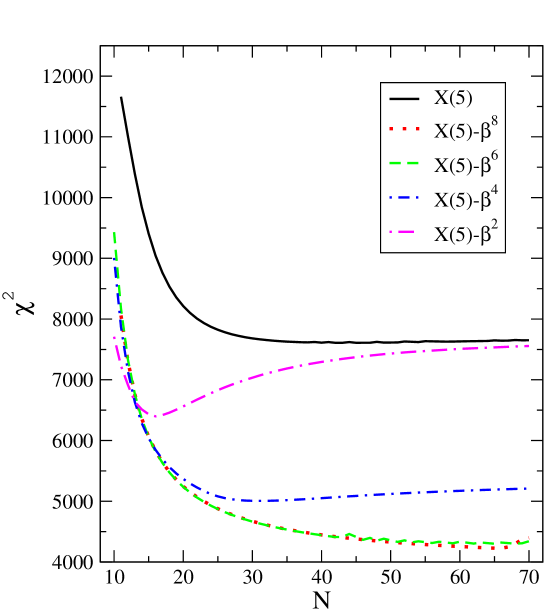
Figure 1: (Color online). $\chi^{2}$ for the IBM fit to the energy levels of the different X(5)-models, as a function of $N$.

II The IBM fit to X(5)-models

II.1 The model

The most general, including up to two-body terms, IBM Hamiltonian can be written in multipolar form as,

$$\hat{H} = \varepsilon_{d}\hat{n}_{d}+\kappa_{0}\hat{P}^{\dagger}\hat{P}+\kappa_{1}\hat{L}\cdot\hat{L}+\kappa_{2}\hat{Q}\cdot\hat{Q}+\kappa_{3}\hat{T}_{3}\cdot\hat{T}_{3}+\kappa_{4}\hat{T}_{4}\cdot\hat{T}_{4}$$ (1)

where $\hat{n}_{d}$ is the $d$ boson number operator, and

$$\hat{P}^{\dagger} = \frac{1}{2}~{}(d^{\dagger}\cdot d^{\dagger}-s^{\dagger}\cdot s^{\dagger}),$$ (2)

$$\hat{L} = \sqrt{10}(d^{\dagger}\times\tilde{d})^{(1)},$$ (3)

$$\hat{Q} = (s^{\dagger}\times\tilde{d}+d^{\dagger}\times\tilde{s})^{(2)}-\frac{\sqrt{7}}{2}(d^{\dagger}\times\tilde{d})^{(2)},$$ (4)

$$\hat{T}_{3} = (d^{\dagger}\times\tilde{d})^{(3)},$$ (5)

$$\hat{T}_{4} = (d^{\dagger}\times\tilde{d})^{(4)}.$$ (6)

The symbol $\cdot$ stands for the scalar product, defined as $\hat{T}_{L}\cdot\hat{T}_{L}=\sum_{M}(-1)^{M}\hat{T}_{LM}\hat{T}_{L-M}$ where $\hat{T}_{LM}$ is the $M$ component of the operator $\hat{T}_{L}$. The operator $\tilde{\gamma}_{\ell m}=(-1)^{m}\gamma_{\ell-m}$ (where $\gamma$ refers to $s$ and $d$ bosons) is introduced to ensure the correct tensorial character under spatial rotations.

Figure 2: (Color online). Parameters (left panels (a), (b) and (c)) and excitation energies (right panels) of the ground (d), beta (e), and gamma (f) bands for the X(5) case, as a function of $N$. In the right panels, the continuous red lines are the X(5) results, while the dashed black lines are the fitted results.

The electromagnetic transitions can also be analyzed in the framework of the IBM. In particular, in this work we will focus on the E2 transitions. The most general E2 transition operator including up to one body terms is written as,

$$\hat{T}^{E2}_{M}=e_{eff}\left[(s^{\dagger}\times\tilde{d}+d^{\dagger}\times\tilde{s})^{(2)}_{M}+\chi(d^{\dagger}\times\tilde{d})^{(2)}_{M}\right],$$ (7)

where $e_{eff}$ is the boson effective charge and $\chi$ is a structure parameter. In this work $\chi$ will be kept fixed to the SU(3) value $-\sqrt{7}/2$.

Although one could use the most general IBM Hamiltonian (1) to describe the X(5)-models a natural question is whether it is possible or not to reduce the number of free parameters. A priori, it is not obvious which terms of the Hamiltonian can be taken out. To answer this question one can rewrite the Hamiltonian (1) in terms of Casimir operators (the definitions for the Casimir operators have been taken from Fran94 ):

$$\hat{H} = \frac{\kappa_{0}}{4}N(N+4)+\big{(}\varepsilon_{d}+\frac{18}{35}\kappa_{4}\big{)}\,\hat{C}_{1}[U(5)]+\frac{18}{35}\kappa_{4}\,\hat{C}_{2}[U(5)]$$ (8)

$$+ \big{(}\kappa_{1}-\frac{3}{8}\kappa_{2}-\frac{\kappa_{3}}{10}-\frac{\kappa_{4}}{14}\big{)}\,\hat{C}_{2}[O(3)]+\frac{\kappa_{2}}{2}\,\hat{C}_{2}[SU(3)]+\big{(}\frac{\kappa_{3}}{2}-\frac{3}{14}\kappa_{4}\big{)}\,\hat{C}_{2}[O(5)]-\frac{\kappa_{0}}{4}\,\hat{C}_{2}[O(6)].$$

It is expected that for the description of the X(5)-models one will need the contribution of the three IBM dynamical symmetry chains. In the Hamiltonian (8) two contributions come from the U(5) algebra, the linear and the quadratic Casimir operators. Therefore, it becomes a reasonable “antsatz” to remove the U(5) quadratic Casimir operator. That implies to fix $\kappa_{4}=0$. Note that its contribution to the rest of Casimir operators is absorbed by the rest of the parameters.

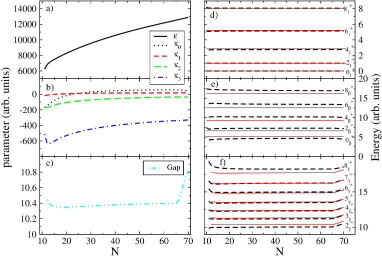
Figure 3: (Color online). Same as Fig. 2 but for the X(5)-$\beta^{8}$ case.

II.2 The fitting procedure

In this section we describe the procedure for getting the IBM Hamiltonian parameters that best fit the different X(5)-models.

The $\chi^{2}$ test is used to perform the fitting. The $\chi^{2}$ function is defined in the standard way,

$$\chi^{2}=\frac{1}{N_{data}-N_{par}}\sum_{i=1}^{N_{data}}\frac{(X_{i}(data)-X_{i}(IBM))^{2}}{\sigma_{i}^{2}},$$ (9)

where $N_{data}$ is the number of data, from a specific X(5)-model, to be fitted, $N_{par}$ is the number of parameters used in the IBM fit, $X_{i}(data)$ is an energy level (or a B(E2) value) taken from a particular X(5)-model, $X_{i}(IBM)$ is the corresponding calculated IBM value, and $\sigma_{i}$ is an arbitrary error assigned to each $X_{i}(data)$.

At this point it is necessary to explain how do we treat the $\gamma$ band head in the X(5) model. The position of this band is not determined by the model, therefore an extra parameter should be introduced for determining the gamma band head, specifically the location of the band head $2_{\gamma}^{+}$ state. Consequently, besides the IBM Hamiltonian parameters, there is this extra free parameter, $\Delta_{\gamma}$, in the fit. This parameter gives the optimum position of the $\gamma$ band in a given X(5)-model for which the best IBM fit is obtained.

In order to perform the fit, we minimize the $\chi^{2}$ function for the energies, using $\varepsilon_{d}$, $\kappa_{0}$, $\kappa_{1}$, $\kappa_{2}$, and $\kappa_{3}$, as free parameters of the IBM Hamiltonian and $\Delta_{\gamma}$ as free parameter for the position of the gamma band head. Note that besides the qualitative argument presented in section II.1 to justify the election of $\kappa_{4}=0$, we have extensively explored other possibilities, as for example $\kappa_{4}\neq 0$ Unpu10 . For this election the improvement in $\chi^{2}$ is not worthy and for some particular cases even affects negatively. In addition, in this case the $\chi^{2}$ function is very flat and the correlation that exists between the free parameters generates non physical oscillations in the value of the fitted parameters. We have also explored the case $\kappa_{3}=0$ and $\kappa_{4}=0$, which produces a important increase in the $\chi^{2}$ value. The $\kappa_{4}=0$ selection produces a smooth and consistent behavior of the fitted parameters, as can be observed in figures 2, 3, 4, 5, and 6.

For doing the fit and the minimization of the $\chi^{2}$ function the MINUIT minuit code has been used. It allows to minimize any multi-variable function.

The labels for the energy levels follow the usual notation introduced for the X(5) model Iach00 : $s$ enumerates the zeroes of the $\beta$ part of the wave function, and $n_{\gamma}$ enumerates the number of $\gamma$ phonons. The set of levels included in the fit for the different X(5)-models are:

• For the ground state band, $s=1,n_{\gamma}=0$, all the states with angular momentum smaller than $10$. An arbitrary $\sigma=0.001$ is used for these states except for the $2_{1}^{+}$ state for which $\sigma=0.0001$ is used. This latter value allows to normalize all the IBM energies to $E(2_{1}^{+})=1$. Note that the energy of the state $2_{1}^{+}$ is fixed arbitrarily to $1$ (remind that the spectrum is calculated up to a global scale factor).

• For the beta band, $s=2,n_{\gamma}=0$, all the states with angular momentum smaller than $10$. An arbitrary $\sigma=0.01$ is used for these states.

• For the $s=3,n_{\gamma}=0$ band, which can be identified with the $\beta\beta$ band, all the states with angular momentum smaller than $10$. An arbitrary $\sigma=0.01$ is used for these states.

• For the gamma band, $s=1,n_{\gamma}=1$, all the states with angular momentum smaller than $9$. An arbitrary $\sigma=0.01$ is used for these states.

With this selection, the number of energy levels included into the fit, $N_{data}$, is equal to $21$. Note that the state $0_{1}^{+}$ is not an actual data to be reproduced because we are interested just in excitation energies and therefore the ground state is naturally fixed to zero in both, X(5)-models and IBM. In Table 1 the states included in the fit are explicitly given.

Band	Error	States
$s=1,n_{\gamma}=0$	$\sigma=0.0001$	$2_{1}^{+}$
	$\sigma=0.001$	$0_{1}^{+},4_{1}^{+},6_{1}^{+},8_{1}^{+}$
$s=2,n_{\gamma}=0$	$\sigma=0.01$	$0_{2}^{+},2_{2}^{+},4_{2}^{+},6_{2}^{+},8_{2}^{+}$
$s=3,n_{\gamma}=0$	$\sigma=0.01$	$0_{3}^{+},2_{3,4}^{+},4_{4}^{+},6_{4}^{+},8_{4}^{+}$
$s=1,n_{\gamma}=1$	$\sigma=0.01$	$2_{4,3}^{+},3_{1}^{+},4_{3}^{+},5_{1}^{+},6_{3}^{+},7_{1}^{+},8_{3}^{+}$

Table 1: States included in the energy fit. In the states labeled with two subindexes, the first one corresponds to X(5), whereas the second to the rest of models.

The ordering index for the even L states in the $\gamma$, $\beta$, and $\beta\beta$ bands is unknown a priori, because of the undetermined position of the X(5)-$\gamma$ bands. However, our best fit always provides a $\gamma$ band above the $\beta$ band, but below the $\beta\beta$ band, that generates the same ordering independently of the particular X(5)-model and number of bosons. The only exception happens for X(5), where the $2^{+}$ of the $\gamma$ band is above the $2^{+}$ state in the $\beta\beta$ band, i.e. they correspond to $2^{+}_{4}$ and $2^{+}_{3}$ respectively.

Once the IBM Hamiltonian is fixed for each X(5)-model by fitting the energy levels, the $\chi^{2}$ function for the B(E2) values is calculated without any additional fitting. The two parameters in the E2 operator (7) are $e_{eff}$, which is fixed to give $B(E2;2_{1}^{+}\rightarrow 0_{1}^{+})=100$, and $\chi$, which is fixed to the SU(3) value $-\sqrt{7}/2$. The computed transitions are enlisted in Table 2. Note that only transitions between states with $n_{\gamma}=0$ states are considered.

	$s_{i}$	$s_{f}$		$s_{i}$	$s_{f}$
$B(E2:2_{1}^{+}\rightarrow 0_{1}^{+})$	1	1	$B(E2:2_{2}^{+}\rightarrow 0_{1}^{+})$	2	1
$B(E2:4_{1}^{+}\rightarrow 2_{1}^{+})$	1	1	$B(E2:2_{2}^{+}\rightarrow 0_{2}^{+})$	2	2
$B(E2:6_{1}^{+}\rightarrow 4_{1}^{+})$	1	1	$B(E2:4_{2}^{+}\rightarrow 2_{1}^{+})$	2	1
$B(E2:8_{1}^{+}\rightarrow 6_{1}^{+})$	1	1	$B(E2:4_{2}^{+}\rightarrow 4_{1}^{+})$	2	1
$B(E2:0_{2}^{+}\rightarrow 2_{1}^{+})$	2	1	$B(E2:4_{2}^{+}\rightarrow 2_{2}^{+})$	2	2
$B(E2:2_{2}^{+}\rightarrow 2_{1}^{+})$	2	1

Table 2: B(E2) transitions to be calculated. $n_{\gamma}=0$ in all the cases.

II.3 The results

We have performed fits of the IBM Hamiltonian (1) parameters plus $\Delta_{\gamma}$ for different values of the number of bosons, $N$, so as to reproduce as well as possible the energies of the states given in Table 1. These states are generated by the different X(5)-models: X(5), X(5)-$\beta^{8}$, X(5)-$\beta^{6}$, X(5)-$\beta^{4}$, and X(5)-$\beta^{2}$.

As mentioned before, $\varepsilon_{d}$, $\kappa_{0}$, $\kappa_{1}$, $\kappa_{2}$, $\kappa_{3}$, and $\Delta_{\gamma}$ are free parameters in a $\chi^{2}$ fit to the energy levels produced by the different X(5)-models ($\kappa_{4}$ was fixed to zero as discussed in the preceding section). In figure 1 the value of the $\chi^{2}$ for the best fit to the different X(5)-models as a function of $N$ is shown. The different lines in figure 1 correspond to the fit to different X(5)-models as stated in the legend box. It is clearly observed that for any $N$ the best agreement is obtained for the X(5)-$\beta^{6}$ and X(5)-$\beta^{8}$ cases, which present a $\chi^{2}$ function almost identical for any value of N. The $\chi^{2}$ function increases for X(5)-$\beta^{4}$ and X(5)-$\beta^{2}$, up to reach X(5) which has the higher $\chi^{2}$ value and therefore the worst degree of agreement. Anyway, the differences between the different X(5)-models are smaller than a factor $2$ in $\chi^{2}$. It is worth noting that these results change slowly with the boson number and in all cases the $\chi^{2}$ function saturates to a given value in the large N limit. The situation presented here is somehow different to the analysis of the $E(5)$-models Garc08 where there is a monotonous behavior in the $\chi^{2}$ values in passing from E(5)-$\beta^{4}$, which presents the lowest value, to E(5)-$\beta^{6}$, E(5)-$\beta^{8}$, and E(5), where the maximum appear.

In figures 2, 3, 4, 5, and 6 the Hamiltonian parameters (panels (a), (b) and (c)) and the excitation energies for the ground (panel (d)), beta (panel (e)) and gamma (panel (f)) bands are plotted for the cases of X(5), X(5)-$\beta^{8}$, X(5)-$\beta^{6}$, X(5)-$\beta^{4}$, and X(5)-$\beta^{2}$, respectively. The Hamiltonian parameters present clear analogies in its behavior in all the X(5)-models. $\varepsilon_{d}$ increases continuously on the whole range of N for all the X(5)-models. $\kappa_{1}$, on the contrary, presents a relatively small and modest value. $\kappa_{0}$ and $\kappa_{2}$ show a very smooth variation till reaching a value of saturation, in all the cases the tendency is to increase, except in the case of $\kappa_{0}$ for X(5)-$\beta^{2}$ which tends to decrease. $\kappa_{3}$ in almost all the cases tends to increase all the way. In the X(5) case, Fig. 2, $\kappa_{3}$ shows up a lowering for small values of N while shows the already commented increasing behavior for larger N values. A similar behavior is also observed for $\Delta_{\gamma}$. Concerning the energy levels, it is remarkable that the plotted energies have almost constant values regardless the value of $N$, except for the $\gamma$ band in the low N region where the energies smoothly move to a saturation value. The agreement for the ground state band is very good but for the $\beta$ and $\gamma$ band the agreement is poorer. In the X(5)-$\beta^{8}$ case, Fig. 3, $\kappa_{3}$ also presents a decreasing behavior for very low values of N, while from there on, it monotonously increases. $\Delta_{\gamma}$ presents an almost constant value, except for the largest values of N, where a increase (look at the small scale) is shown. Regarding the energies, they remain almost constant in the full range of $N$, except for the $\gamma$ band, where, the increase of the $\Delta_{\gamma}$ value generates, for large values on N, a corresponding increasing. The agreement of the energies in the ground state band is perfect and reasonable in the $\beta$ and $\gamma$ bands.

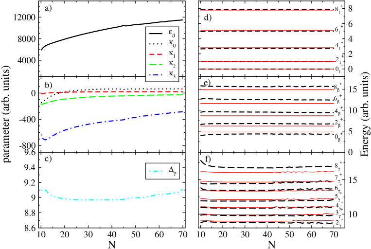
Figure 4: (Color online). Same as Fig. 2 but for the X(5)-$\beta^{6}$ case.

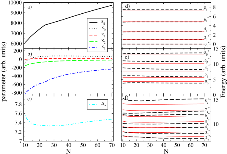
Figure 5: (Color online). Same as Fig. 2 but for the X(5)-$\beta^{4}$ case.

The X(5)-$\beta^{6}$ case, Fig. 4, is very similar to X(5)-$\beta^{8}$, although here $\Delta_{\gamma}$ presents a rather flat behavior with a minimum around $N=40$. Once more, the agreement of the energies in the ground state band is perfect and reasonable in the $\beta$ and $\gamma$ bands. The X(5)-$\beta^{4}$ case shown in Fig. 5 presents a monotonous increase of $\kappa_{3}$ and a behavior for $\Delta_{\gamma}$ almost identical to X(5)-$\beta^{6}$. Here also the agreement of the energies in the ground state band is good while the description of the $\beta$ and $\gamma$ bands is poorer.

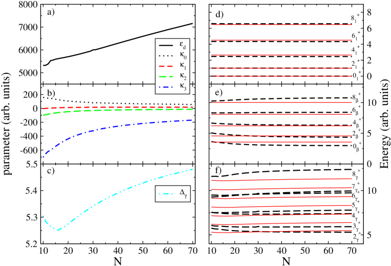
Figure 6: (Color online). Same as Fig. 2 but for the X(5)-$\beta^{2}$ case.

Finally, X(5)-$\beta^{2}$, Fig. 6, also presents a monotonous increase of $\kappa_{3}$ whereas $\kappa_{0}$ has a smooth decreasing behavior till a saturation value. In $\Delta_{\gamma}$ the behavior of X(5) is recovered, with a smooth decrease up to $N=15$ and an smooth increase from there on. The agreement of the energies in the ground state band is very good and reasonable for the $\beta$ and $\gamma$ bands.

In panels (e) of Figs. 2, 3, 4, 5, and 6 one can see that the moment of inertia of the $\beta$ band increases from X(5), where it reaches the smallest value, till X(5)-$\beta^{2}$ where it is maximum. In panels (d) and (f) of these figures one can also observe how the moment of inertia of ground and $\gamma$ bands is roughly stable for all the models. This tendency is correctly reproduced by the IBM fits.

It is worth remarking that the agreement of the energies in the $\beta$ and the $\gamma$ bands is not clearly deteriorated when ascending up in the band. In particular, in the $\gamma$ band the best agreement is obtained for angular momenta values 4, 5, 6. Similar conclusions are obtained for the $\beta\beta$ band. This fact has a important consequence for the value of $\chi^{2}$ and supposes that, contrary to expected, the higher states included in the fitting procedure for the $\beta$, $\gamma$, and $\beta\beta$ bands produce smaller contributions to $\chi^{2}$ than the low lying states of these bands.

To have a clearer idea of the values of the Hamiltonian parameters obtained in the fits we present in Table 3 the parameters of the IBM Hamiltonians that best fit the different X(5)-models for N=50. Two facts are apparent, first the parameters for X(5)-$\beta^{8}$ and X(5)-$\beta^{6}$ are amazingly similar and, second the parameters change almost monotonously when going from X(5) to X(5)$-\beta^{2}$.

	$\varepsilon_{d}$	$\kappa_{0}$	$\kappa_{1}$	$\kappa_{2}$	$\kappa_{3}$	$\Delta_{\gamma}$
X(5)	15420	-31.7	7.5	-77.1	-454.8	17.5
X(5)$-\beta^{8}$	11426	53.6	17.8	-43.3	-369.2	10.4
X(5)$-\beta^{6}$	10661	58.5	19.9	-38.5	-372.7	9.2
X(5)$-\beta^{4}$	8942	72.9	19.6	-27.8	-301.4	7.4
X(5)$-\beta^{2}$	6595	65.9	18.2	-17.6	-216.6	5.4

Table 3: Parameters (in arbitrary units) of the IBM Hamiltonian plus the excitation energy for the $\gamma$ band head, $\Delta_{\gamma}$, that best fit the different X(5)-models for N=50.

As a test for the produced wave functions with the fitted IBM Hamiltonian, they are used for calculating E2 transition probabilities, B(E2). The effective charge in the E2 operator (7) is fixed so as to give $B(E2;2_{1}^{+}\rightarrow 0_{1}^{+})=100$, thus no free parameters are left in this calculation. For the B(E2)’s calculated (not a fit) a $\chi^{2}$ value has been obtained for each X(5)-model with an arbitrary $\sigma=10$. In figure 7 the corresponding $\chi^{2}$ value is plotted as a function of $N$ for all the X(5)-models considered. Figure 7 shows a smooth dependence of $\chi^{2}$ on $N$. The $\chi^{2}$ value decreases monotonically as $N$ increases for all the X(5)-models. The best agreement is obtained for X(5) while the worst is for X(5)-$\beta^{2}$.

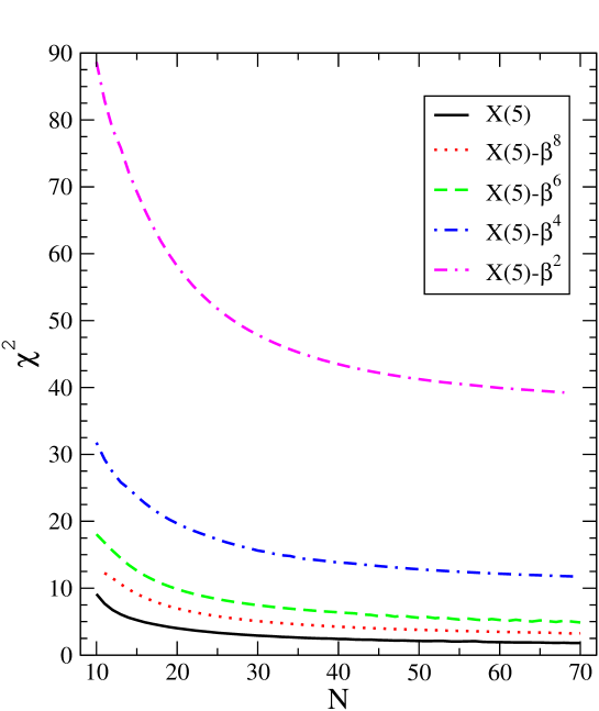
Figure 7: (Color online). $\chi^{2}$ values for the E2 transition rates for the different X(5)-models, as a function of $N$, calculated using the IBM electromagnetic transition operator $\hat{T}^{E2}_{M}=e_{\mbox{eff}}\big{[}(s^{\dagger}\tilde{d}+d^{\dagger}\tilde{s})-\sqrt{7}/2(d^{\dagger}\times\tilde{d})^{(2)}_{M}$ ].

For a quantitative comparison, the B(E2) values for selected transitions with $N=50$ are shown in Table 4. In this table, it is clear the remarkable agreement between the IBM calculations and those from the X(5) model. However as soon as we move to the rest of models the agreement starts getting worse. Some comments on these results are in order. First, one observes that the B(E2)’s within the ground state band are calculated qualitatively correct in all models. This agreement is quantitatively good for the X(5) case and gets worse for the other models. The X(5)-$\beta^{2}$ case is the worst, showing differences of a factor of 2 for some transitions. The IBM seems to saturate to a too small value as the angular momentum increases, therefore the deviation increases with the angular momentum. The intraband transitions in the $\beta$ band exhibit the same kind of agreement, where the larger discrepancy is for $B(E2:4_{2}^{+}\rightarrow 2_{2}^{+})$. The interband transitions once more agree well qualitatively. In summary, one can say that the structure of the wave functions is correctly captured by the IBM fit, specially for X(5), and the calculations are able to reproduce the sequence of large/small values (with few exceptions), confirming the appropriated structure of the wave functions.

	X(5)	IBM	X(5)-$\beta^{8}$	IBM	X(5)-$\beta^{6}$	IBM	X(5)-$\beta^{4}$	IBM	X(5)-$\beta^{2}$	IBM
$B(E2:2_{1}^{+}\rightarrow 0_{1}^{+})$	100.0	100.0	100.0	100.0	100.0	100.0	100.0	100.0	100.0	100.0
$B(E2:4_{1}^{+}\rightarrow 2_{1}^{+})$	159.9	155.4	163.4	159.1	165.3	145.7	169.0	164.9	177.9	174.6
$B(E2:6_{1}^{+}\rightarrow 4_{1}^{+})$	198.2	181.6	208.8	189.2	214.6	160.8	226.2	199.9	255.2	217.7
$B(E2:8_{1}^{+}\rightarrow 6_{1}^{+})$	227.6	199.1	247.3	210.3	258.1	166.2	279.9	224.9	337.1	249.2
$B(E2:0_{2}^{+}\rightarrow 2_{1}^{+})$	62.4	43.4	74.7	55.7	81.0	11.2	93.2	74.6	121.9	106.7
$B(E2:2_{2}^{+}\rightarrow 2_{1}^{+})$	8.2	4.4	9.7	7.3	10.3	0.9	11.3	15.4	13.4	33.4
$B(E2:2_{2}^{+}\rightarrow 0_{1}^{+})$	2.1	0.2	2.2	0.0	2.2	3.5	2.0	0.6	1.6	4.4
$B(E2:2_{2}^{+}\rightarrow 0_{2}^{+})$	79.5	56.1	97.2	67.5	106.0	68.3	122.0	69.3	155.7	49.2
$B(E2:4_{2}^{+}\rightarrow 2_{1}^{+})$	0.9	0.2	0.8	0.0	0.7	5.2	0.5	0.7	0.1	2.1
$B(E2:4_{2}^{+}\rightarrow 4_{1}^{+})$	6.1	3.4	7.7	6.8	8.4	0.7	9.6	16.6	12.4	27.7
$B(E2:4_{2}^{+}\rightarrow 2_{2}^{+})$	120.0	111.9	149.1	121.7	162.9	108.1	187.7	110.9	240.3	99.3

Table 4: B(E2) values (in arbitrary units) obtained, for $N=50$, for the fitted IBM Hamiltonians (see text) compared with those provided by the different X(5)-models.

III The critical Hamiltonian

One of the most attractive features of the X(5)-models treated in this work is that they are supposed to describe, at different approximation levels, the critical point in the transition from spherical to rigid axially deformed shapes. Since they are connected to a given IBM Hamiltonian, as shown in the preceding section, this should correspond to the critical point in the transition from spherical to axially deformed shapes, i.e. this Hamiltonian should produce an energy surface with degenerated spherical and deformed minima. Is this the case for the fitted IBM Hamiltonians obtained in the preceding section? Before starting with the discussion it is necessary to establish a measure on how close is a given IBM Hamiltonian to the critical point.

An energy surface can be associated to a given IBM Hamiltonian by using the intrinsic state formalism Gino80b ; Diep80a ; Diep80b which introduces the shape variables $(\beta,\gamma)$ in the IBM. To define the intrinsic state one has to consider that the dynamical behavior of the system can be approximately described in terms of independent bosons moving in an average field Duke84 . The ground state of the system is written as a condensate, $|c\rangle$, of bosons that occupy the lowest-energy phonon state, $\Gamma_{c}^{\dagger}$:

$$|c\rangle=\frac{1}{\sqrt{N!}}(\Gamma^{\dagger}_{c})^{N}|0\rangle,$$ (10)

where

$$\Gamma^{\dagger}_{c}=\frac{1}{\sqrt{1+\beta^{2}}}~{}\left(s^{\dagger}+\beta\cos\gamma\,d^{\dagger}_{0}+\frac{1}{\sqrt{2}}~{}\beta\sin\gamma\,(d^{\dagger}_{2}+d^{\dagger}_{-2})\right).$$ (11)

$\beta$ and $\gamma$ are variational parameters related with the shape variables in the geometrical collective model Gino80b . The expectation value of the Hamiltonian (1) in the intrinsic state (10) provides the energy surface of the system, $E(N,\beta,\gamma)=\langle c|\hat{H}|c\rangle$. This energy surface in terms of the parameters of the Hamiltonian (1) and the shape variables can be readily obtained Isac81 (note that we keep the $\kappa_{4}$ variable for completeness),

$$\langle c|\hat{H}|c\rangle = {\displaystyle{\frac{N\beta^{2}}{(1+\beta^{2})}}}\Bigl{(}\varepsilon_{d}+6\,\kappa_{1}-\frac{9}{4}\,\kappa_{2}+\frac{7}{5}\,\kappa_{3}+\frac{9}{5}\,\kappa_{4}\Bigr{)}$$

$$+ {\displaystyle{\frac{N(N-1)}{{{(1+\beta^{2})}^{2}}}}}\Big{[}\frac{\kappa_{0}}{4}+\beta^{2}(-\frac{\kappa_{0}}{2}+4\,\kappa_{2})+2\,{\sqrt{2}}\,\beta^{3}\,\kappa_{2}\,\cos(3\,\gamma)$$

$$+\beta^{4}(\frac{\kappa_{0}}{4}+\frac{\kappa_{2}}{2}+\frac{18}{35}\,\kappa_{4})\Big{]}.$$ (12)

The shape of the nucleus is defined through the equilibrium value of the deformation parameters, $\beta$ and $\gamma$, which are obtained minimizing the ground state energy, $\langle c|\hat{H}|c\rangle$. A spherical nucleus has a global minimum in the energy surface at $\beta=0$, while a deformed one has the absolute minimum at a finite value of $\beta$. The parameter $\gamma$ represents the departure from axial symmetry, i.e. $\gamma=0$ and $\gamma=\pi/3$ stand for an axially deformed nucleus, prolate and oblate respectively, while any other value corresponds to a triaxial shape. An additional situation appears when the energy surface is independent on $\gamma$ but shows a minimum at a finite value of $\beta$, in this case the nucleus is $\gamma$-unstable. It has to be noted that for a general IBM Hamiltonian including up to two body terms, as the one considered in this work, triaxiality is forbidden.

With the tools described above one can study phase transitions in the IBM Diep80a . First, the parameters that define the Hamiltonian are the control parameters and are usually chosen in such a way that only one of them is a variable, while the rest remain constant. The deformation parameters $\beta$ and $\gamma$ become the order parameters, although in our case the order parameter is just $\beta$. Roughly speaking, a phase transition appears when there exists an abrupt change in the shape of the system when changing smoothly the control parameter. The phase transitions can be classified according to the Ehrenfest classification Stan71 . First order phase transitions appear when there exists a discontinuity in the first derivative of the energy with respect to the control parameter. This discontinuity appears when two degenerate minima exist in the energy surface for two values of the order parameter $\beta$. Second order phase transitions appear when the second derivative of the energy with respect to the control parameter displays a discontinuity. This happens when the energy surface presents a single minimum for $\beta=0$ and the surface satisfies the condition ${\left(\frac{d^{2}E}{d\beta^{2}}\right)_{\beta=0}}=0$. In a modern classification, second order phase transitions belongs to the high order or continuous phase transitions Stan71 . The X(5) situation was designed to describe first order phase transitions.

To determine whether a given Hamiltonian corresponds to a critical point or not, the flatness or the existence of two degenerate minima in the energy surface should be investigated. For the case of one parameter IBM Hamiltonian, e.g. Consistent Q (CQF) Hamiltonians Warn82 , it is simple to find an analytical expression for the critical control parameter in the Hamiltonian. However, for a general IBM Hamiltonian, as the one used in this work, it is necessary to rewrite the energy surface in a special way, as proposed first by López-Moreno and Castaños in Ref. Lope96 . There, the authors manage to write the energy surface of a general IBM Hamiltonian in terms of two parameters. They made use of some concepts from the Catastrophe Theory Gilm81 to define the two essential parameters, ($r_{1},r_{2}$) of the problem. In terms of these two essential parameters they found expressions for the locus, in the essential parameter space, that gives a critical point at the origin in $\beta$, called bifurcation set, and for the locus that gives rise to two degenerate minima, called Maxwell set. The essential parameters $r_{1}$ and $r_{2}$ can be written as,

$$r_{1}=\frac{a_{3}-u_{0}+\tilde{\varepsilon}/(N-1)}{2a_{1}+\tilde{\varepsilon}/(N-1)-a_{3}},$$ (13)

$$r_{2}=-\frac{2a_{2}}{2a_{1}+\tilde{\varepsilon}/(N-1)-a_{3}},$$ (14)

where

$$\tilde{\varepsilon} = \varepsilon_{d}+6\,\kappa_{1}-{9\over 4}\,\kappa_{2}+{7\over 5}\,\kappa_{3}+{9\over 5}\,\kappa_{4}$$

$$a_{1} = {1\over 4}\,\kappa_{0}+{1\over 2}\,\kappa_{2}+{18\over 35}\,\kappa_{4}$$

$$a_{2} = 2\,\sqrt{2}\,\kappa_{2}$$

$$a_{3} = -{1\over 2}\,\kappa_{0}+4\,\kappa_{2}$$

$$u_{0} = {\kappa_{0}\over 2}.$$ (15)

Using the essential parameters, the energy surface can be written as:

$$E^{*}(\beta,\gamma) = \frac{\langle c|\hat{H}|c\rangle-N(N-1)u_{0}/2}{N(N-1)(2a_{1}+\tilde{\varepsilon}/(N-1)-a_{3})}$$ (16)

$$= \frac{1}{1+\beta^{2}}(\beta^{4}+r_{1}\beta^{2}(\beta^{2}+2)-r_{2}\beta^{3}cos3\gamma).$$

Note that $E^{*}(\beta,\gamma)$ does not depend on the number of bosons, allowing to compare fairly energy surfaces corresponding to different boson numbers.

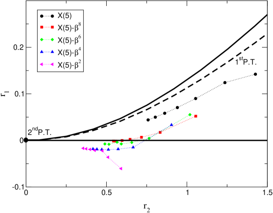
Figure 8: (Color online). Position in the plane $r_{1}-r_{2}$ of the energy surfaces extracted from the fitted IBM Hamiltonians to the different X(5) models as a function of $N$ (10, 20, 30, 40, 50, 60, and 70). The largest value of N is placed on the left hand side whereas the smallest one is on the right part of the figure.

In figure 8 we display the plane of the essential parameters where the fitted Hamiltonians to the different X(5)-models are plotted with different symbols. In this plane a critical first order Hamiltonian corresponds to a point over the dashed line (Maxwell set, i.e. two degenerated minima). The $r_{1}=0$ corresponds to $\left(\frac{d^{2}E}{d\beta^{2}}\right)_{\beta=0}=0$, i.e. to the appearance of the spherical minimum (antispinodal point). The curved full line above the Maxwell set corresponds to $\left(\frac{d^{2}E}{d\beta^{2}}\right)_{\beta_{0}}=0$, with $\beta_{0}\neq 0$, i.e. it corresponds to the appearance of a deformed minimum (spinodal point). The area below the curved full line and above $r_{1}=0$ is the coexistence region. In this region two minima, one spherical and one deformed, coexist. We also represent in the plane the second order critical point ($r_{1}=r_{2}=0$). Note that all the points above the dashed line correspond to spherical shapes, while those below that line represent deformed shapes. We only plot the $r_{2}>0$ semi plane because our IBM Hamiltonian always corresponds to prolate shapes and therefore to $r_{2}>0$. The semi plane $r_{2}<0$ is identical to the presented in figure 8, but for oblate shapes. The different symbols in the figure correspond to the IBM Hamiltonians fitted to one of the X(5) models (see legend) for N ranging from 10 to 70. The idea is to see if in the large N limit the obtained IBM Hamiltonians go to the Maxwell set (dashed line) that is the line of first order phase transitions. For all the models, the N value of the different points increases from the right to the left.

Several important features can be extracted from this figure. The main one is that the X(5) case, for the whole range of $N$, is always very close to the Maxwell set, i.e. to the first order phase transition line, being closer as the value of $N$ increases. This is not exactly the case for the rest of fits. X(5)-$\beta^{8}$, X(5)-$\beta^{6}$, and X(5)-$\beta^{4}$ seat on the coexistence region for small or moderate N values, but they go towards the prolate deformation region as $N$ increases, although they are always very close to the antispinodal line. Finally, the case X(5)-$\beta^{2}$ lies on the deformed region but it approaches to the coexistence area as N increases. In general, one observes that the mapped IBM energy surfaces moves further away from the coexistence region as one changes from X(5) through X(5)-$\beta^{8}$, X(5)-$\beta^{6}$, X(5)-$\beta^{4}$, and X(5)-$\beta^{2}$. In general, the higher the value of n is (X(5)-$\beta^{n}$), the closer to the coexistence region is the IBM energy surface. In all the cases one observes that the different models always move in the direction of the second order phase transition point as N increases.

In order to illustrate graphically the shapes of the energy surfaces obtained with the different IBM Hamiltonians, we plot in figure 9 the axial IBM energy surfaces $E^{*}(\beta,0)$ (eq. 16), along the prolate leg, extracted from the fit to the five analyzed X(5)-models as a function of the deformation $\beta$ for three values of N: 10, 40, and 70. All the panels show a rather similar aspect, for N=10 there exist a more pronounced minimum, while passing from N=40 to N=70 the energy surface flattens, moving into a shape with two approximately degenerated minima. As it was studied in figure 8, in panel a), which is for X(5), the three curves present two minima, in panels b), c), and d), corresponding to X(5)-$\beta^{8}$, X(5)-$\beta^{6}$, and X(5)-$\beta^{4}$, respectively, only the line for N=10 has two minima, while N=40 and N=70 show only a deformed minimum (see insets of figure 9). Finally, panel e) is for X(5)-$\beta^{2}$, and the three curves present only a deformed minimum, although it clearly flattens as N increases. This analysis confirms that X(5)-models map into IBM Hamiltonians that are very close to the first order phase transition line, but the closest Hamiltonian to the transition area is the one mapped from the original X(5) model.

A somehow similar analysis to the one presented in this section was performed in Mccu05 ; Mccu06 . There, the authors studied the connection between X(5) and X(5)-$\beta^{2}$ using a two parameter IBM Hamiltonian (they also analyzed X(3)) for $N=10$. Their conclusion was that the X(5) case is close to, although not exactly at, the first order phase transition region for a finite number of boson. This conclusion is very similar to the one extracted from our results. For the case of X(5)-$\beta^{2}$ their results are similar to the X(5) case, i.e. the corresponding IBM Hamiltonian is even closer to the first order phase transition line that in the X(5) case. These later results are also in agreement with the conclusions raised in the present work, although we have found that X(5)-$\beta^{2}$ is further from the coexistence region than X(5). The origin of the discrepancy should be based on the more restricted set of data used in Mccu05 ; Mccu06 in their fits and the smaller number of parameters used in the IBM Hamiltonian.

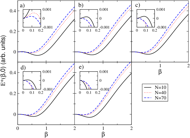
Figure 9: (Color online). IBM axial energy surfaces, for prolate shapes (see eq. 16) as a function of $\beta$, for selected values of $N$ (see text for definition). a) X(5), b) X(5)-$\beta^{8}$, c) X(5)-$\beta^{6}$, d) X(5)-$\beta^{4}$, and e) X(5)-$\beta^{2}$. In the insets a closer view of the region around $\beta=0$ are shown.

IV Summary and conclusions

In this paper, we have studied the connection between the X(5)-models and the IBM on the basis of a numerical mapping between these models. To establish the mapping we have performed a best fit of the general IBM Hamiltonian to a selected set of energy levels produced by several X(5)-models; as an additional parameter we have used the energy of the gamma band head, which is not fixed by the X(5)-models. Later on, a free parameter check of the wave functions, obtained with the best fit parameters, has been done by calculating relevant B(E2) transition rates. All calculations have been done as a function of the number of bosons. Once the best fit IBM Hamiltonians to the different X(5)-models are obtained, their energy surfaces are constructed and analyzed with the help of the Catastrophe Theory so as to know how close they are to a critical point.

We have shown that it is possible, in all cases, to obtain a mapping between the X(5)-models and the IBM with a reasonable agreement for both energies and B(E2) transition rates. In general, the goodness of the fit to the energies and B(E2) transition rates is independent on the number of bosons. Globally, the agreement is similar for all the models: for the energies the best agreement is for X(5)-$\beta^{8}$ and X(5)-$\beta^{6}$ while the worst is for X(5). Anyway, the $\chi^{2}$ values obtained that give the goodness of the fits are comparable for all the models. Additional tests have been done to the produced wave functions by calculating B(E2) transition rates. No free parameters are included in these calculations. In this case, the best agreement (smallest $\chi^{2}$ value) is obtained for X(5) while the worst is for X(5)-$\beta^{2}$. A consequence of this good general agreement is that it would be almost impossible, from an experimental point of view, to discriminate between a X(5)-model and its corresponding IBM Hamiltonian when only few low-lying states are considered (usually the four lowest states in the ground, beta, and gamma bands.)

We have also proved that the X(5) model corresponds to an IBM Hamiltonian which is very close to the first order phase transition region, getting closer for larger values of $N$. X(5)-$\beta^{8}$, X(5)-$\beta^{6}$, and X(5)-$\beta^{4}$ models seat on the coexistence region for small and moderate values of $N$, but they slightly move into the deformed region for the larger values of $N$. Finally X(5)-$\beta^{2}$ stands all the way in the deformed region, although very close to the coexistence region. In all the cases the system evolves towards the second order critical point as N increases.

It is worth mentioning that the conclusions raised in this work are somehow dependent on the constrains imposed in the fitting procedure. On one hand we have checked that the inclusion, or not, of high lying states in the bands considered in the fit does not strongly affect to the results. On the other hand we have extensively checked the case with $\kappa_{4}\neq 0$ Unpu10 . This later case generates values of $\chi^{2}$ similar to the ones presented in this work, but the global picture of the mapped IBM Hamiltonians to the X(5)-models is not so consistent as one the shown here. In particular, the change of the Hamiltonian parameters as a function of N or as a function of the considered X(5)-model is not smooth enough. There are instabilities in the fitting procedure due to the fact that the produced $\chi^{2}$ surface is very flat.

Finally, it is worth mentioning the differences between the X(5)-models/IBM and the E(5)-models/IBM mapping Garc08 . For the E(5)-models the agreement for both, the energies and the B(E2) transition rates is really remarkable and much better than for the X(5)-models. Globally, the best agreement is obtained for the E(5)-$\beta^{4}$ Hamiltonian and the worst for the E(5) case. For the case of very large number of bosons the only E(5)-model that can be reproduced exactly by the IBM is E(5)-$\beta^{4}$, corresponding such a Hamiltonian with the critical point of the model ($r_{1}=0$) (as shown in Aria03 ; Garc05 ). All the E(5)-models correspond to IBM Hamiltonians very close to the critical area, $|r_{1}|<0.05$ with $r_{2}=0$. Therefore, one can say that the E(5)-models are appropriate to describe transitional $\gamma-$unstable regions close to the critical point. However, not all the X(5)-models are suitable for describing the critical area between the axially deformed and the spherical shapes, only X(5) is really appropriated to this end. Finally, for the E(5)-models it is observed the existence of something similar to a quasidynamical symmetry Rowe04a , we call this phenomenon quasi-critical point symmetry. In the case of the X(5)-models we cannot talk about quasi-critical point symmetry because the agreement between IBM and the X(5)-models is not good enough, only in the case of the ground state band for X(5) we have the appropriated agreement to say that a quasi-critical point symmetry is present.

V Acknowledgements

This work has been partially supported by the Spanish Ministerio de Educación y Ciencia and by the European regional development fund (FEDER) under projects number FIS2008-04189, FPA2007-63074, by CPAN-Ingenio and by the Junta de Andalucía under projects FQM160, FQM318, P05-FQM437 and P07-FQM-02962.

References

- (1) J.E. García-Ramos and J.M. Arias, Phys. Rev. C 77, 054307 (2008).
- (2) A. Bohr, Mat. Fys. Medd. Dan. Vidensk. Selsk. 26 (14) (1952).
- (3) A. Bohr and B.R. Mottelson, Mat. Fys. Medd. Dan. Vidensk. Selsk. 27 (16) (1953).
- (4) A. Bohr and B.R. Mottelson, Nuclear Structure, vol. II, (Benjamin, Elmsford, NY, 1969).
- (5) A. Arima and F. Iachello, Ann. Phys. 99, 253 (1976).
- (6) A. Arima and F. Iachello, Ann. Phys. 111, 201 (1978);
- (7) O. Scholten, F. Iachello, and A. Arima, Ann. Phys. 115, 325 (1978);
- (8) F. Iachello and A. Arima, The interacting boson model (Cambridge University Press, Cambridge, 1987).
- (9) A.E.L. Dieperink, O. Scholten, F. Iachello, Phys. Rev. Lett. 44, 1747 (1980).
- (10) A.E.L. Dieperink and O. Scholten, Nucl. Phys. A 346, 125 (1980).
- (11) J.N. Ginocchio, M.W. Kirson, Phys. Rev. Lett. 44, 1744 (1980).
- (12) J.N. Ginocchio, M.W. Kirson, Nucl. Phys. A 350, 31 (1980).
- (13) M.W. Kirson, Ann. Phys. (N.Y.) 143, 448 (1982).
- (14) J.N. Ginocchio, Nucl. Phys. A 376, 438 (1982).
- (15) D.J. Rowe and G. Thiamova, Nucl. Phys. A 760, 59 (2005).
- (16) E. López-Moreno and O. Castaños, Phys. Rev. C 54, 2374, (1996).
- (17) J.M. Arias, J. Dukelsky, J.E. García-Ramos, and J. Vidal, Phys. Rev. C 75, 014301 (2007).
- (18) D.J. Rowe, P.S. Turner, and G. Rosensteel, Phys. Rev. Lett. 93, 232502 (2004).
- (19) D.J. Rowe, Nucl. Phys. A 745, 47 (2004).
- (20) P.S. Turner and D.J. Rowe, Nucl. Phys. A 756, 333 (2004).
- (21) G. Thiamova and D. J. Rowe, Eur. Phys. J. A 41, 189 (2009).
- (22) D.L. Hill and J.A. Wheeler, Phys. Rev. 89, 1102, (1953).
- (23) J.M. Eisenberg and G. Greiner, Nuclear models, (North-Holland, American Elsevier, 1970).
- (24) D. Janssen, R.V. Jolos, and F. Dönau, Nucl. Phys. A 224, 93 (1974).
- (25) M. Moshinsky, Nucl. Phys. A 338, 156 (1980)
- (26) A. Klein and M. Vallieres, Phys. Lett. B 98, 5 (1981).
- (27) A. Klein, C-T. Li, and M. Vallieres, Phys. Rev. C 25, 2733 (1982).
- (28) H.J. Assenbaum and A. Weiguny, Z. Phys. A 310, 75 (1983).
- (29) P. Van Isacker, Phys. Rev. Lett. 83, 4269 (1999).
- (30) F. Iachello, Phys. Rev. Lett. 85, 3580, (2000).
- (31) F. Iachello, Phys. Rev. Lett. 87, 052502, (2001).
- (32) F. Iachello, Phys. Rev. Lett. 91, 132502, (2003).
- (33) R.F. Casten and N.V. Zamfir, Phys. Rev. Lett. 85, 3584, (2000).
- (34) R.F. Casten and N.V. Zamfir, Phys. Rev. Lett. 87, 052503 (2001).
- (35) R.F. Casten and E.A. McCutchan, J. Phys. G 34, R285 (2007) and references therein.
- (36) P. Cejnar, J. Jolie, and R.F. Casten, Rev. Mod. Phys., in press.
- (37) P.G. Bizzeti and A.M. Bizzeti-Sona, Phys. Rev. C 70, 064319 (2004).
- (38) P.G. Bizzeti and A.M. Bizzeti-Sona, Phys. Rev. C 77, 024320 (2008).
- (39) D. Bonatsos, D. Lenis, N. Minkov, D. Petrellis, and P. Yotov, Phys. Rev. C 71, 064309 (2005).
- (40) D. Bonatsos, D. Lenis, N. Minkov, P.P. Raychev, and P.A. Terziev, Phys. Rev. C 69, 014302 (2004).
- (41) D. Bonatsos, D. Lenis, D. Petrellis, P.A. Terziev, and I. Yigitoglu, Phys. Lett. B 632, 238 (2006).
- (42) E.A. McCutchan, N.V..Zamfir, and R.F. Casten, Phys. Rev. C 71, 034309 (2005).
- (43) E.A. McCutchan, D. Bonatsos, and N.V..Zamfir, Phys. Rev. C 74, 034306 (2006).
- (44) D. Bonatsos, et al., Phys. Rev. C 76, 064312 (2007).
- (45) D. Bonatsos, D. Lenis, E.A. McCutchan, D. Petrellis, and I. Yigitoglu, Phys. Lett. B 649, 394 (2007).
- (46) M.A. Caprio, Phys. Rev. C 72, 054323 (2005).
- (47) A. Frank and P. Van Isacker, Algebraic Methods in Molecular and Nuclear Structure Physics (John Wiley & Sons, NY, 1994).
- (48) F. James, Minuit: Function Minimization and Error Analysis Reference Manual, Version 94.1, CERN, 1994.
- (49) J. Barea et al., unpublished.
- (50) J. Dukelsky, G.G. Dussel, R.P.J. Perazzo, S.L. Reich, and H.M. Sofia, Nucl. Phys. A 425,93 (1984).
- (51) P. Van Isacker and J.Q. Chen, Phys. Rev. C 24, 684 (1981).
- (52) H.E. Standley, Introduction to phase transitions and critical phenomena, Oxford University Press, Oxford (1971).
- (53) D.D. Warner and R.F. Casten, Phys. Rev. Lett. 48, 1385 (1982).
- (54) R. Gilmore, Catastrophe theory for scientists and engineers (Wiley, New York, 1981).
- (55) J.M. Arias, C.E. Alonso, A. Vitturi, J.E. García-Ramos, J. Dukelsky, and A. Frank, Phys. Rev. C 68, 041302(R) (2003).
- (56) J.E. García-Ramos, J. Dukelsky, and J.M. Arias, Phys. Rev. C 72, 037301 (2005).
- (57) D.J. Rowe, Phys. Rev. Lett. 93, 122502 (2004).