Current-induced torques in the presence of spin-orbit coupling

Abstract

In systems with strong spin-orbit coupling, the relationship between spin-transfer torque and the divergence of the spin current is generalized to a relation between spin transfer torques, total angular momentum current, and mechanical torques. In ferromagnetic semiconductors, where the spin-orbit coupling is large, these considerations modify the behavior of the spin transfer torques. One example is a persistent spin transfer torque in a spin valve: the spin transfer torque does not decay away from the interface, but approaches a constant value. A second example is a mechanical torque at single ferromagnetic-nonmagnetic interface.

Introduction— Since the prediction bergerdw ; slonc ; berger of spin transfer torques in non-collinear ferromagnetic metal circuits, they have been the subject of extensive research ralph ; miltat . The possibility of using spin transfer torque to improve the commercial viability of magnetic random access memory (MRAM) katine , and the rich non-equilibrium physics involved establish the topic as one of practical and fundamental interest. These torques arise from the exchange interaction between non-equilibrium, current-carrying electrons and the spin-polarized electrons that make up the magnetization. In systems where the spin-orbit coupling is weak, the torque on the magnetization can be computed from the change in the spins flowing through the region containing the magnetization. This relation is a consequence of conservation of total spin. Here, we consider systems in which the spin-orbit coupling cannot be neglected (and hence total spin is no longer conserved).

In systems where spin angular momentum is not conserved, the relationship between the spin transfer torque and the flow of spins needs to be generalized. Conservation of total angular momentum implies that mechanical torques on the lattice of the material accompany changes in the magnetization richardson ; einstein . This effect has been used for decades to measure the $g$-factor of metals. More recent theoretical mohanty ; kovalev and experimental guiti work considers the current-induced mechanical torques present at the interface of a ferromagnet and non-magnet, similar in spirit to the spin transfer torques on the magnetization present in spin valves.

In this article we develop a theory for current-induced torques (both spin transfer torques and mechanical torques) in systems with strong spin-orbit coupling, and apply it to a model of dilute magnetic semiconductors. We find that by accounting for the orbital angular momentum of the electrons, we can relate the change in total angular momentum flow to spin transfer torques and mechanical torques. We study two system geometries where these torques play important roles. The first is a spin-valve geometry, which is used to study the features of spin transfer torques in the presence of spin-orbit coupling. The second is a single interface between a ferromagnet and non-magnet, which elucidates the physics underlying current-induced mechanical torques.

Formalism — We consider a Hamiltonian consisting of a spin-independent kinetic and potential energy $H_{0}=\frac{-\hbar^{2}\nabla^{2}}{2m}+V({\bf r})$, an exchange splitting $\Delta$, and an atomic-like spin-orbit interaction parameterized by $\alpha$:

$$H = H_{0}+\frac{\Delta}{\hbar}\frac{\left({\bf M}\cdot\hat{\bf s}\right)}{M_{s}}+\frac{\alpha}{\hbar^{2}}\left(\hat{\bf L}\cdot\hat{\bf s}\right),$$ (1)

where $\hat{\bf L}$ and $\hat{\bf s}$ are the electron angular momentum and spin operators, respectively footnote1 . The exchange splitting arises from a magnetization ${\bf M}$, with magnitude $M_{s}$. We treat the magnetization within mean field theory.

We consider the torque on the magnetization due to electric current flow. The spin transfer torque $\bm{\tau}_{\rm STT}$ at position ${\bf r}$ from electronic states with spin density ${\bf s}({\bf r})$ is proportional to the component of spin transverse to the magnetization nunez : $\bm{\tau}_{\rm STT}({\bf r})=\frac{d{\bf M}({\bf r})}{dt}=\frac{-\Delta}{\hbar^{2}}\left({\bf M({\bf r})}\times{\bf s({\bf r})}\right)$. In the absence of spin-orbit coupling, this torque can be related to the divergence of a spin current, which offers conceptual and computational simplicity stiles . In the following we analyze how spin-orbit coupling changes this simple result. One consequence is an expression for the mechanical torque $\bm{\tau}_{\rm lat}$.

We develop an expression for $\bm{\tau}_{\rm STT}$ by evaluating the time-dependence of the electron spin and angular momentum densities. To do so, we adopt a Heisenberg picture of time evolution, and evaluate $\frac{d\hat{O}({\bf r})}{dt}=\frac{i}{\hbar}\left[H,\hat{\psi}^{\dagger}({\bf r})\hat{O}\hat{\psi}({\bf r})\right],$ where $\hat{\psi}({\bf r})$ is the position operator, for the operators $\hat{O}={\bf\hat{s}}$, ${\bf\hat{L}}$. This procedure leads to ralph :

$$\frac{d{\bf\hat{s}}}{dt}=\nabla\cdot\hat{\bf Q}_{\bf s}({\bf r})-\hat{\bm{\tau}}_{\rm STT}+\frac{\alpha}{\hbar^{2}}\left(\hat{\bf L}\times\hat{\bf s}\right)$$ (2)

where $\hat{\bf Q}_{\bf s}({\bf r})=\hat{\psi}^{\dagger}({\bf r}){\hat{\bf v}}\otimes{\bf{\hat{s}}}\hat{\psi}({\bf r})$, and the velocity operator is given by ${\bf{\hat{v}}}=\frac{i\hbar}{2m}\left(\overleftarrow{\nabla}-\overrightarrow{\nabla}\right)$; here the arrow superscript specifies the direction in which the gradient acts. In addition:

$$\frac{d{\bf\hat{L}}}{dt}=\nabla\cdot\hat{\bf Q}_{\bf L}({\bf r})-\hat{\bm{\tau}}_{\rm lat}+\frac{\alpha}{\hbar^{2}}\left(\hat{\bf s}\times\hat{\bf L}\right)$$ (3)

where $\hat{\bf Q}_{\bf L}({\bf r})=\hat{\psi}^{\dagger}({\bf r})\frac{1}{2}\left({\hat{\bf v}}{\bf{\hat{L}}}+{\hat{\bf L}}{\bf{\hat{v}}}\right)\hat{\psi}({\bf r})$ (the product of non-commuting operators ${\bf{\hat{L}}}$ and ${\bf{\hat{v}}}$ is symmetrized). We’ve defined $\hat{\bm{\tau}}_{\rm lat}({\bf r})=\frac{i}{\hbar}\hat{\psi}^{\dagger}({\bf r})\left[H_{0},{\bf{\hat{L}}}\right]\hat{\psi}({\bf r})$, which is nonzero for a potentials $V({\bf r})$ which break rotational symmetry footnote2 .

We define a total angular momentum $\hat{\bf J}=\hat{\bf L}+\hat{\bf s}$, a total angular momentum current $\hat{\bf Q}_{\bf J}=\hat{\bf Q}_{\bf L}+\hat{\bf Q}_{\bf s}$, and combine Eqs. (2) and (3) to obtain:

$$\frac{d\hat{\bf J}}{dt}-\bm{\nabla}\cdot\hat{\bf Q}_{\bf J}=-\hat{\bm{\tau}}_{\rm STT}-\hat{\bm{\tau}}_{\rm lat}.$$ (4)

Finally, we take the expectation value of Eqs. (2-4), replacing operators by densities. Eq. (4) is our main formal result. When spin-orbit coupling is important, the total angular momentum in the conduction electrons couples both to the magnetization and the lattice. The coupling of electron spin to the lattice requires both spin-orbit coupling and crystal field potential. The term $\bm{\tau}_{\rm lat}$ changes the physical picture of spin transfer torque substantially, as is illustrated by considering Eq. (4) for a single bulk eigenstate: $\frac{d{\bf J}}{dt}$ and $\nabla\cdot{\bf Q_{\bf J}}$ vanish, however $\bm{\tau}_{\rm STT}$ and $\bm{\tau}_{\rm lat}$ may both be non-zero, implying a coupling from the angular momentum of the lattice to the magnetization. This coupling flows from the lattice to the orbital subsystem through the crystal field, which then couples to the spin through spin-orbit coupling, and finally to the magnetization through the exchange interaction.

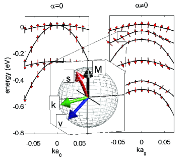
Figure 1: Left and right panels shows GaMnAs band structure without and with spin-orbit, respectively (for $\gamma_{2}=\gamma_{3}=2.4$). (arrows indicate spin direction of eigenstates). The inset shows the direction of bulk magnetization, and spin, velocity, and k vectors for a single state (in black, red, blue, and green). The torque from the misalignment between magnetization and spin equals the torque from the misalignment between velocity and k vectors.

Application to DMS — We apply this general formalism to a model of a dilute magnetic semiconductor (DMS). DMSs are semiconductor host materials which become ferromagnetic when doped with magnetic atoms. ${\rm Ga_{1-x}Mn_{x}As}$ is the archetype for these materials, and can be described as a system of local moments of ${\rm Mn}$ $d$-electrons, whose interaction is mediated by holes in the semiconductor valence band jungwirth . The valence states are described by the Kohn-Luttinger Hamiltonian $H_{0}^{\rm KL}$, which represents a small-${\bf k}$ expansion for a periodic $H_{0}$, acting in the $\ell=1$ subspace (describing valence states). It is given by:

$$H_{0}^{\rm KL} = \frac{\hbar^{2}}{2m}\left(\left(\gamma_{1}+4\gamma_{2}\right)k^{2}-\frac{6\gamma_{2}}{\hbar^{2}}\left({\bf L}\cdot{\bf k}\right)^{2}\right.$$ (5)

$$\left.-\frac{6}{\hbar^{2}}\left(\gamma_{3}-\gamma_{2}\right)\sum_{i\neq j}k_{i}k_{j}L_{i}L_{j}\right),$$

where ${\bf L}$ are the spin-1 matrices for the $p$-state orbitals, $\gamma_{1},~{}\gamma_{2},~{}\gamma_{3}$ are Luttinger parameters, and ${\bf k}$ is the Bloch wave-vector. Figure 1 shows how the presence of spin-orbit coupling affects the band structure.

For periodic systems the velocity operator can be written as: ${\bf{\hat{v}}}=\frac{1}{\hbar}\frac{\partial H}{\partial{\bf k}}$, and spin and angular momentum current densities are again defined as symmetrized products of ${\hat{\bf v}}$ and ${\hat{\bf L}}$, and ${\hat{\bf v}}$ and ${\hat{\bf s}}$. The dynamics of the magnetization occur on a much longer time scale than that of the electronic states, so we compute the dynamics from a sum over scattering states, for which $\frac{d{\bf s}}{dt}=\frac{d{\bf L}}{dt}=0$. For the Luttinger Hamiltonian, the $z$-component of $\bm{\hat{\tau}}_{\rm lat}$ is:

$${\hat{\tau}}_{\rm lat}^{z} = \left({\hat{\bf v}}\times\hbar{\bf k}\right)_{z}+\frac{6(\gamma_{2}-\gamma_{3})}{\hbar m}\left\{\left(k_{x}L_{y}+k_{y}L_{x}\right),\right.$$ (6)

$$~{}~{}~{}~{}~{}~{}~{}~{}~{}~{}~{}~{}~{}~{}~{}~{}~{}~{}~{}~{}~{}\left.\left(k_{x}L_{x}-k_{y}L_{y}\right)\right\}~{}~{}~{}~{}$$

where the brackets on the second term indicate an anticommutator. Other components are given by cyclic permutation of indices. The first term of Eq. (6) can be written as ${\hat{\bf v}}\times\hbar{\bf k}=\frac{d}{dt}\left({\hat{\bf r}}\times\hbar{\bf k}\right)$. This term can be interpreted as a torque on the crystal angular momentum ${\hat{\bf r}}\times\hbar{\bf k}$, and results from the misalignment between wave vector and velocity. It is generically nonzero for any material with a non-spherical Fermi surface. In the spherical approximation ($\gamma_{2}=\gamma_{3}$), Eq. (4) implies that the net flux of total angular momentum into a volume is equal to the change of magnetization plus the crystal angular momentum inside the volume.

STT in spin-valves — We first consider a system to study the $\bm{\tau}_{\rm STT}$ term of Eq. (4). Figure 2(a) shows the geometry; current flows in the $\hat{z}$-direction, perpendicular to the magnetization of both layers. We focus on the component of torque which is in the plane spanned by the two magnetization directions. This in-plane torque is determined by the out-of-plane (or $\hat{z}$-component) spin density nunez . For the results presented here, we use the parameter values: $(\gamma_{1},\gamma_{2},\gamma_{3})=(6.85,2.1,2.9)$, $\Delta=0.27~{}{\rm eV}$, $\alpha=0.11~{}{\rm eV}$, $E_{\rm F}=0.16~{}{\rm eV}$ ($E_{\rm F}$ is measured from the top of the valence band). The tunnel barrier is described by Eqs. (1) and (5), with $\Delta=0$, and with an energy offset so that the top of the valence band is 0.1 eV below $E_{\rm F}$. We calculate the eigenstates numerically and apply boundary conditions as described in Ref. malik .

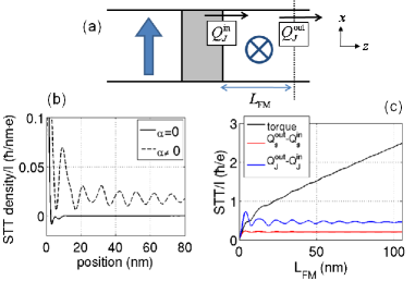
Figure 2: (a)Spin valve geometry: FM layers’ magnetization points in the $\hat{x}$ and $\hat{y}$ (out-of-page) directions. (b) The spin transfer torque versus position away from the left normal metal-FM interface, which decays to zero in the absence of spin-orbit coupling, and does not in its presence. (c) Plot of the total spin transfer torque, the net flux of spin current, and net flux of total angular momentum current versus FM thickness. The linear dependence for large thickness is due to a persistent spin transfer torque.

Figure 2(b) shows the spin transfer torque density as a function of distance away from the interface. We find that for $\alpha=0$ (no spin-orbit coupling), the torque decays to zero away from the interface, as expected stiles . For $\alpha\neq 0$, the torque oscillates around a nonzero value, and extends into the bulk. Figure 2(c) shows that the total spin transfer torque as a function of ferromagnetic (FM) layer thickness $L_{\rm FM}$ is proportional to thickness for large $L_{\rm FM}$. This is in contrast to the metallic spin valve, where the torque is an interface effect and becomes constant for large $L_{\rm FM}$.

This persistent spin transfer torque arises because the spins of individual eigenstates are not aligned with the magnetization (see Fig. 1) in the presence of spin-orbit coupling. The misalignment gives rise to a torque between the lattice and the magnetization. In equilibrium, these torques cancel when summed over all occupied states. However, the presence of a current changes the occupation of the bulk states and can give rise to a torque manchon ; garate in systems without inversion symmetry. Inversion symmetry is only very weakly broken in bulk GaMnAs, and is not included in the Kohn Luttinger Hamiltonian, Eq. (5). Here, interfaces between materials breaks inversion symmetry.

The combination of an interface and a current flow changes the occupation of the bulk states near the Fermi energy (depending on the transmission probabilities of individual states across the interface) and induces coherence between these states. The change in the occupation probabilities gives rise to a persistent transverse spin accumulation, which only decays through other scattering mechanisms not included here (e.g. defect scattering). This spin accumulation gives rise to the persistent spin transfer torque. The coherence between the states modifies the spin accumulation and the torque near the interface but these corrections decay away from the interface due to dephasing.

Figure 3 shows, as a function of the spin-orbit coupling constant $\alpha$, the values of total spin transfer torque, the angular momentum current flux, -$\bm{\tau}_{\rm lat}$, and the persistent contribution to spin transfer torque (for $L_{\rm FM}=30~{}{\rm nm}$). We determine the persistent contribution from the slope of the integrated total versus FM width $L_{\rm FM}$ at large $L_{\rm FM}$ (see Fig. 2c). This procedure neglects the contributions from coherence near the interface. In this example, the spin transfer torque increases with the addition of spin-orbit coupling, largely because of the addition of the persistent term. This qualitative behavior depends on system parameters: for $E_{\rm F}=0.34~{}{\rm eV}$, for example, the spin-orbit coupling decreases the total torque.

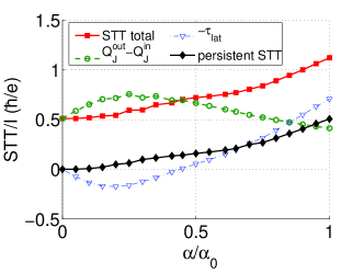
Figure 3: The total spin transfer torque, the net flux of total angular momentum, $-\bm{\tau}_{\rm lat}$, and the persistent component of the spin transfer torque on a FM layer with $L_{\rm FM}=30~{}{\rm nm}$ as $\alpha$ is increased from 0 to $\alpha_{0}=0.11~{}{\rm eV}$.

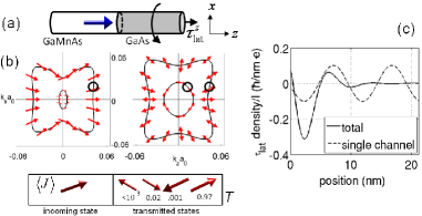
Figure 4: (a) shows the system geometry. We take electron particle flow from left to right, and consider the mechanical torque $\bm{\tau}_{\rm lat}$ in the z direction. (b) shows slices of the Fermi surface for the different layers, with $\langle{\bf J}({\bf k})\rangle$ superimposed, and also shows the ${\bf J}$-character of the states specified by the black circle. Also shown is the transmission probability for each of the states in the GaAs. (c) shows the total mechanical torque density in the GaAs as a function of distance from the interface (dark curve), and the contribution from the single incoming state specified in (b) (dashed curve).

Nanomechanical torques in wires — We next consider a system which exemplifies that physics of the $\bm{\tau}_{\rm lat}$ term of Eq. (4): a single interface between GaMnAs and GaAs, with the direction of the magnetization parallel to the current flow (see Fig. 4a). This is similar to the geometry considered in previous theoretical and experimental work mohanty ; kovalev ; guiti . The vanishing magnetization in GaAs implies $\bm{\tau}_{\rm STT}=0$, so that $\bm{\tau}_{\rm lat}=\nabla\cdot{\bf Q}_{\bf J}$, and its total value can be deduced from ${\bf Q}_{\bf J}^{\rm in}-{\bf Q}_{\bf J}^{\rm out}$. We use the same parameters as before, except $E_{\rm F}=0.06~{}{\rm eV}$, and the top of the valence band of both layers coincide.

Figure 4c shows $\bm{\tau}_{\rm lat}$ in the GaAs layer as a function of distance away from the interface (assuming electron particle flow from left to right). The total torque (dark curve) shows oscillatory decay, while the torque from a particular channel (light curve) shows simple oscillation. The behavior of the single channel is illustrated in Fig. 4b. We assume specular scattering, so that the incident state chosen (black circle) transmits into the four states of GaAs with equal $k_{x},~{}k_{y}$ (also shown with black circles). The character of these states, along with the transmission probability, is shown in Fig. 4b. The incoming state couples most strongly to the state with similar ${\bf J}$ character, but also partially transmits into other states with different ${\bf J}$ character and wave vector $k_{z}$. These different scattering channels interfere with each other, leading to an oscillatory ${\bf J}(z)$, with an oscillation period inversely proportional to the splitting of $k_{z}$ wave-vectors of the different sheets of the Fermi surface. This splitting is from the lattice crystal field and spin-orbit coupling, the agents responsible for $\bm{\tau}_{\rm lat}$. Different channels have different oscillation periods, so that their total decays away from the interface, as happens for spin transfer torques in ferromagnets stiles . For the parameters used here, we find $Q_{J^{z}}^{\rm in}=1.20\hbar\frac{I}{e}$, due to the polarization of the states from the magnetization, while $Q_{J^{z}}^{\rm out}=0.46\hbar\frac{I}{e}$. Mechanisms not considered here, such as spin-flip scattering, ensure that $Q_{J^{z}}^{\rm out}$ decays to zero away from the interface.

The mechanical torque is $Q_{J^{z}}^{\rm in}-Q_{J^{z}}^{\rm out}=0.74\hbar\frac{I}{e}$. For appropriate experimental conditions, this torque is greater than the thermal fluctuations and is a measurable effect. We refer the reader to Ref. mohanty ; kovalev ; guiti for details of treatment of the torsion dynamics and experimental details. The formalism developed here generalizes previous work to allow for microscopic evaluation of the electronic structure contribution to the current-induced mechanical torque. For systems with nonzero magnetization, the microscopic form of $\bm{\tau}_{\rm lat}$ is necessary to determine the partitioning of total angular momentum flux between torques on the magnetization and torques on the lattice. Our theory neglects other mechanisms of spin relaxation, such as disorder-induced spin-flip scattering, so that full calculations will require microscopic calculations like these to be embedded in diffusive transport calculations.

Conclusion— We have shown how atomic-like spin-orbit coupling affects current-induced torques: both the spin transfer torque on the magnetization and the mechanical torque on the lattice. In GaMnAs spin valves, we find a contribution to the spin transfer torque that persists throughout the bulk. This result may explain experiments which find critical currents which are up to an order of magnitude smaller than the value expected from a simple accounting of the net spin current flux chiba ; elsen . For a single interface between GaMnAs and GaAs, we microscopically compute the mechanical torque due to scattering from the interface. These results highlight important, qualitatively different physics at play when spin-orbit coupling is strong.

The authors acknowledge helpful conversations with A. H. MacDonald.

References

- (1) L. Berger, J. Appl. Phys. 3, 2156 (1978); ibid. 3, 2137 (1979).
- (2) J. Slonczewski, J. Magn. Magn. Mat. 62, 123, (1996).
- (3) L. Berger, Phys. Rev. B 54, 9353 (1996).
- (4) D. C. Ralph and M. D. Stiles, J. Magn. Magn. Mater. 320, 1190 (2007).
- (5) M. D. Stiles and J. Miltat, Top. Appl. Phys. 101, 225 (2006).
- (6) J. A. Katine and E. E. Fullerton, J. Magn. Magn. Mater. 320, 1217 (2007).
- (7) O. W. Richardson, Phys. Rev. 26, 248 (1908).
- (8) A. Einstein and A. de Hass, Verhandlungen der Deutschen Physikalischen Gesellschaft, 17, 152 (1915).
- (9) P. Mohanty et al., Phys. Rev. B 70, 195301 (2004).
- (10) A. A. Kovalev et al., Phys. Rev. B 75, 014430 (2007).
- (11) G. Zolfagharkhani et al., Nature Nanotech. 3, 720 (2008).
- (12) In addition to atomic-like angular momentum, there is a contribution to the total orbital angular momentum from itinerant motion through the lattice. The distinction between “local” and “itinerant” orbital angular momentum is discussed in Ref. vanderbilt . In this work, we consider only the atomic-like contribution.
- (13) T. Thonhauser et al., Phys Rev. Lett. 95, 137205 (2005).
- (14) A. S. Núñez and A. H. MacDonald, Solid State. Comm. 139, 31 (2006).
- (15) M. D. Stiles and A. Zangwill, Phys. Rev. B 66, 014407 (2002).
- (16) For , our definition of is equivalent to . We use in anticipation of other forms of , in particular the form of the Luttinger Hamiltonian.
- (17) T. Jungwirth et al., Rev. Mod. Phys. 78, 809 (2006).
- (18) A. M. Malik et al., Phys. Rev. B 59, 2861 (1999).
- (19) A. Manchon and S. Zhang, Phys. Rev. B 78, 212405 (2008).
- (20) Ion Garate and A. H. MacDonald, Phys. Rev. B 80, 134403 (2009).
- (21) D. Chiba et al., Phys. Rev. Lett. 93, 216602 (2004).
- (22) M. Elsen et al., Phys. Rev B 73, 035303 (2006).