Bayesian Segmentation of Oceanic SAR Images: Application to Oil Spill Detection

Abstract

This paper introduces Bayesian supervised and unsupervised segmentation algorithms aimed at oceanic segmentation of SAR images. The data term, i.e., the density of the observed backscattered signal given the region, is modeled by a finite mixture of Gamma densities with a given predefined number of components. To estimate the parameters of the class conditional densities, a new expectation maximization algorithm was developed. The prior is a multi-level logistic Markov random field enforcing local continuity in a statistical sense. The smoothness parameter controlling the degree of homogeneity imposed on the scene is automatically estimated, by computing the evidence with loopy belief propagation; the classical coding and least squares fit methods are also considered. The maximum a posteriori segmentation is computed efficiently by means of recent graph-cut techniques, namely the $\alpha$-Expansion algorithm that extends the methodology to an optional number of classes. The effectiveness of the proposed approaches is illustrated with simulated images and real ERS and Envisat scenes containing oil spills.

I Introduction

A wide number of oceanic phenomena become visible on SAR images as they have distinct scattering characteristics, namely the sea surface roughness and thus the normalized radar cross section (NRCS). Among these phenomena are gravity waves, convective cells, oceanic internal waves, current and coastal fronts, eddies, upwelling processes, ship wakes and oil pollution [1]. The automatic detection of these signatures is of outmost interest for a panoply of ocean monitoring systems, both for security, for commercial and for research applications. An example of an automated ocean feature detection scheme, able to detect fronts, ice edges and polar lows, is described in [2]. Another example is the Ocean Monitoring Workstation (OMW), developed by the company Satlantic. Usually, the first two steps of the processing chains of such systems are segmentation followed by classification. The Segmentation step computes a set of regions defining an image partition, where the features of each region, for example the gray levels, are similar in some sense. The classification focus then on each region attaching a label to it. For example, oil spill detection based on SAR images has bee approached by many authors with the referred to classification-segmentation scheme(see for example [3]); the SAR image is first segmented and then the classification is focused on the regions with lower scattering; the classifier then computes a number of features from these regions including shape, moments, scale parameters, etc. [3] based on which a decision on whether the region corresponds to oil or look-alike is taken. We should refer, however,

An application where segmentation of oceanic SAR images is important is oil spill detection. In fact, many approaches to this issue have been proposed in recent years. Most of them follow the described segmentation-classification structure, although other methods exist that do not, like for example kernel-based anomaly detectors [4]. A review of SAR segmentation techniques for oil spill detection can be found in [3]. The present work, which is an elaboration of our previous works [5], [6], [7], describes algorithms for the segmentation of dark signatures in oceanic SAR images, following a Bayesian approach. The adopted technique uses as data model a finite Gamma mixture, with a given predefined number of components, for modeling each class density. In fact, this density is well suited to filtered intensity SAR images as shown, e.g., in [8] and in [9]. By using a mixture, we aim at describing the continuous backscattering variability that may be observed in the SAR sea data. Moreover, a mixture is able to describe densities presenting more than one maximum, as it is the case of oceanic multi-look SAR images histograms. This cannot be achieved by none of the statistical models for SAR intensities proposed in the literature, like for example any of the Pearson distributions.

In this work we propose two supervised and one unsupervised algorithm. The supervised algorithms demand an interaction with the user that manually selects a region containing pixels from the dark signature of interest and a region containing water pixels. These regions should be representative and can be made up of different not connected parts. The unsupervised algorithm is an improvement of the supervised ones and is completely automatic.

To estimate the parameters of the class conditional densities, a new expectation maximization (EM) algorithm was developed. Details are described in appendix. When segmenting small sub-scenes of the image, a simplified data model with only one Gamma function per class can be used.

The prior used to impose local homogeneity is a multi-level logistic (MLL) model Markov random field (MRF) [10], with 2nd order neighborhood. To infer the prior smoothness parameter controling the degree of scene homogeneity, we develop an EM algorithm that uses loopy believe propagation (LBP) [11]. We have also exploited different classic estimation methods, namely the least squares fit (LSF) and the coding method (CD) (see [10] for details) for comparison.

To infer the labels, we adopt the maximum a posterior (MAP) criterion, which we implement efficiently and exactly with graph-cut techniques [12].

Although the segmentation of oceanic dark patches is typically based on the assumption of two classes, we have generalized the problem to an optional number of classes. The underlying integer optimization problem is now attacked with the graph-cut based $\alpha$-Expansion algorithm [13].

To evaluate the accuracy of the proposed algorithms, different simulations addressing both the referred Gamma model as well as intensity images corrupted with Gaussian noise have been carried out for error rate assessment.

The algorithms have also been applied to real SAR images containing well documented oil spills. For doing so, the scenes are divided in tiles and segmented individually.

I-A Related Work

Related approaches to the problem of oil spill segmentation are built on off-the-shelf segmentation algorithms such as the adaptive image thresholding and the hysteresis thresholding. Entropy methods based on the maximum descriptive length (MDL) and wavelet based approaches have also been proposed. Another recently proposed segmentation methodology applies Hidden Markov Chains (HMC) to a multiscale representation of the original image. Hereby the wavelet coefficients are statistical characterized by the Pearson system and by the the generalized Gaussian family [14]. When other SAR products are available, for example polarimetric data, other methods have been described in the literature, like constant false alarm rate filters [15].

An example of an elaborated adaptive thresholding technique is provided by [16]. In this method, an image pyramid is created by averaging pixels in the original image. From the original image, the next level in the pyramid is created with half the pixel size of the original image. A threshold is then computed for each level based on local estimates of the roughness of the surrounding sea and on a look-up table containing experimental values obtained from a training data set.

Hysteresis thresholding has been used as the base for detecting oil slicks in [17]. The method includes two steps: applying a so-called directional hysteresis thresholding (DHT) and performing the fusion of the DHT responses using a Bayesian operator. The MDL technique, which basically consists in applying information theory in order to find the image description which has the lowest complexity, has been applied in [18] to segment speckled SAR images, namely those containing oil slicks. This segmentation method describes the image as a polygonal grid and determines the number of regions and the location of the nodes that delimit the regions. The two-dimensional wavelet transform, used as a bandpass filter to separate processes at different scales, has also been adopted to oil slick detection in the framework of an algorithm for automated detection and tracking of mesoscale features from satellite imagery. [2].

I-B Contributions

We approach oil spill segmentation using a Bayesian framework and a multi-level Logistic (MLL) prior. Several methods in the same vein have been proposed since the seminal work of Geman and Geman [19], see e.g., [20]. Applications of these ideas in the segmentation of SAR images can be found, e.g., in [21], [22], [23].

The main contributions of this work to the state-of-art in oil spill segmentation are the following:

• the development of an EM algorithm to estimate the parameters of a mixture of a pre-defined number of Gamma distributions, in order to model the intensities in a SAR image

• the development of an EM algorithm using LBP to estimate the smoothness parameter in the MRF used as pior in our framework

• the application of recent graph-cut techniques for solving the energy minimization problem that arises from the followed Bayesian methodology.

• the design of a semisupervised algorithm for oil spill segmentation supported on the tools referred to above.

I-C Paper Organization

The article is organized as follows: Section 1 introduces the problem, with references to related work and giving the main contributions of the present work; Section 2 overviews the Bayesian methodology that builds the base to the proposed algorithms. In addition, it briefly reviews the concept of the $\alpha$-Expansion technique that has been implemented to generalize the methodology to an optional number of classes; Section 3 describes the used parameter estimation techniques; Section 4 describes the supervised segmentation algorithms; Section 5 describes the unsupervided algorithm and Section 6 presents results of segmenting simulated and real images applying the algorithms proposed in Section 4 and 5; Finally Section 7 contains the main conclusions and future work remarks. The article also includes an appendix where the referred to EM algorithm, developed to estimate the parameters of the class conditional densities of the Gamma mixture data model, is described.

II Problem Formulation

II-A Bayesian Approach

let ${\cal L}:=\left\{1,\ldots,c\right\}$ be a set of $c$ classes and ${\cal P}:=\left\{1,2,\ldots,N\right\}$ be the set of $N$ pixels (sites) where measurements $y:=\left\{y_{1},y_{2},\ldots,y_{N}\right\}$, the SAR intensities, are available. A labeling $x:=\left\{x_{1},x_{2},\ldots x_{N}\right\}$ is a mapping from ${\cal P}$ to ${\cal L}$, i.e., it assigns to each pixel $p\in{\cal P}$ a label $x_{p}\in{\cal L}$. Any labeling $x$ can be uniquely represented by a partition of image pixels $P=\left\{{P_{l}|l\in{\cal L}}\right\}$, where $P_{l}=\left\{p\in{\cal P}|x_{p}=l\right\}$ is the subset of pixels to which the label $l$ have been assigned. Since there is an one-to-one correspondence between labelings $x$ and partitions $P$, we use these notions interchangeably. By applying a segmentation algorithm to the image y, we get $\hat{x}:=\left\{\hat{x}_{1},\hat{x}_{2}\ldots\hat{x}_{N}\right\}$, where $\hat{x}_{i}$ is the inferred label for pixel $i\in{\cal P}$.

II-B Observation Model

In our problem formulation, we assume conditional independence of the measurements given the labels, i.e.,

$$p(y|x)=\prod_{i=1}^{N}p(y_{i}|x_{i})=\prod_{l=1}^{c}\prod_{i\in{\cal P}_{l}}p(y_{i}|\phi^{l}),$$ (1)

where $p(\cdot|\phi^{l})$ is the density corresponding to class $l$ and $\phi_{l}$ the correspondent vector of parameters. The adopted density is a finite Gamma mixture given by

$$p(y_{i}|\phi^{l})=\sum_{s=1}^{K}\alpha_{s}^{l}\,p(y_{i}|\theta_{s}^{l}),$$ (2)

where $K$ is the number of Gamma modes in the mixture, $i$ indexes the pixel, and, for the class $l$, $\theta_{s}^{l}$ is the vector of parameters of the Gamma mode $s$, and $\alpha_{s}^{l}$ is the a priori probability of mode $s$. We denote $\theta^{l}:=(\theta_{1}^{l},\dots,\theta_{K}^{l})$, $\alpha^{l}:=\left(\alpha_{1}^{l},\ldots,\alpha_{K}^{l}\right)$, and $\phi^{l}:=(\alpha^{l},\theta^{l})$.

Given that $p(y_{i}|\theta_{s}^{l})$ is Gamma distributed, we have then

$$p\left(y_{i}|\theta_{s}^{l}\right)=\frac{(\lambda_{s}^{l})^{a_{s}^{l}}}{\Gamma\left(a_{s}^{l}\right)}y_{i}^{a_{s}^{l}-1}\exp{\left(-\lambda_{s}^{l}y_{i}\right)},\hskip 14.22636pt,$$ (3)

where $\theta_{s}^{l}:=\left(a_{s}^{l},\lambda_{s}^{l}\right)$. The mean and variance of a random variable with the density (3) is, respectively, $a_{s}^{l}/\lambda_{s}^{l}$ and $a_{s}^{l}/(\lambda_{s}^{l})^{2}$.

The mixture parameters $\theta^{l}$ are estimated from the data by applying the EM Gamma mixture estimation algorithm described in Appendix. The procedure is the same both for the supervised and for the unsupervised algorithms.

We now make a brief comment on our choice of the Gamma mixture for modeling the observation densities. Under the assumption of fully developed speckle, the complex radar amplitude is zero-mean circular Gaussian distributed [24]. The average intensity computed over a number of independent random variables with the same density is, thus, Gamma distributed. It happens, however, that in sea SAR imaging one or more of the above assumptions may fail, rendering the Gamma density a poor model for SAR intensity [14]. A line of attack to obtain better models is to use more flexible parametric families, such as the Pearson System [25, Ch. 4.1] (see also [9]). However, in our problem each class density exhibits much more variability than that of accommodated by the the Pearson System. We have very often, for example, multi-modal densities. We should resort, therefore, to a mixture of Pearson System densities, what would lead to complex learning procedures. We have experimentally observed, however, that the Gamma mixture yields very good fittings for real SAR histograms, obtained with a moderately complex learning algorithm. For this reason, we have adopted the Gamma mixture model.

II-C Prior

A second assumption we are making is of local smoothness of the labels in a statistical sense. It is more likely to have neighboring sites with the same label than the other way around. We model this local smoothness with a second order MRF, $P\left(x\right)$; more specifically, by an MLL model (Ising model in the case of two classes). The Markov property assumes that

$$p\left(x_{i}|~{}x_{j},j\in{\cal P}\right)=p\left(x_{i}|~{}x_{j},j\in{\cal N}_{i}\right),$$ (4)

where ${\cal N}_{i}$ is the set of neighbors of site $i$. If $p\left(x_{i}|~{}x_{j},j\in{\cal N}_{i}\right)>0$, then the Hammersley-Clifford Theorem states that $p(x)$ has the form of the Gibbs distribution

$$p\left(x\right)=\frac{1}{{\cal Z}}\exp^{-U\left(x\right)},$$ (5)

where ${\cal Z}$ is the so called partition function and $U$ is the energy function

$$U\left(x\right)=\sum_{cl\in C}V_{cl}\left(x\right),$$ (6)

where $C$ is the set of cliques and $V_{cl}\left(x\right)$ is the clique potential defined over clique $cl$. In this work, we have pair-wise cliques defined on a second-order neighborhood (8 pixels). That is, $C=\{(i,j)\,:i\in{\cal N}_{j},\;j\in{\cal N}_{i},\;i>j\}$.

In these conditions, the MLL clique potentials, in the isotropic case, is given by

$$V_{cl}\left(x_{r},x_{s}\right)=-\beta\delta\left(x_{r}-x_{s}\right),$$ (7)

where $r,s\in cl$, $\delta(x):=I_{0}(x)$ is the indicator function of set $\{0\}$, and parameter $\beta>0$ controls the degree of scene homogeneity.

II-D Maximum a Posteriori Estimate

The posterior of the labeling given the observed data is

$$p\left(x|y\right)\propto p\left(y|x\right)p\left(x\right).$$ (8)

In order to infer $x$, we adopt the MAP criterion. This amounts to maximize the posterior density of the labeling given the observed data:

$$\hat{x}=\arg\max_{x}p\left(x|y\right),$$ (9)

and is equivalent to minimize the negative logarithm of (8). In this sense, we may rewrite the problem in the following way:

$$\hat{x}=\arg\min_{x}E(x_{1},\dots,x_{n}),$$ (10)

where

$$E\left(x_{1},\ldots,x_{N}\right)=-\log p(x|y)+c^{te},$$ (11)

and $c^{te}$ denotes an irrelevant constant. From equation (8), we have

$$E\left(x_{1},\ldots,x_{N}\right)=\sum_{p=1}^{N}E^{i}\left(x_{i}\right)+\sum_{i,j\in cl}E^{i,j}\left(x_{i},x_{j}\right),$$ (12)

with

$$E^{i}\left(x_{i}\right) = -\log p\left(y_{i}|x_{i}\right)$$ (13)

$$E^{i,j}(x_{i},x_{j}) = -\beta\delta(x_{i}-x_{j}).$$ (14)

II-E Energy Minimization

As already stated, we are concerned with the minimization of $E\left(x_{1},\ldots x_{N}\right)$ given by (12), which we term energy. For two classes, (i.e., $c=2$), the global minimum of $E\left(x_{1},\ldots x_{N}\right)$ can be computed exactly by applying the graph-cut algorithm described in [12]. This is a consequence of energy being graph-representable, i.e., $E^{i,j}\left(0,0\right)+E^{i,j}\left(1,1\right)\leq E^{i,j}\left(0,1\right)+E^{i,j}\left(1,0\right)$ (for details see [12]). For more than two classes, the solution of (9) can be approximately computed by the $\alpha$-Expansion technique [13], also based on graph-cut concepts. This algorithm finds the local minimum of the energy within a known factor of the global minimum.

We now give a brief description of the $\alpha$-Expansion algorithm. Given a label $\alpha$, a move from a partition $P$ (with correspondent labeling $x$) to a new partition $P^{\prime}$ (with correspondent labeling $x^{\prime}$) is called an $\alpha$-Expansion if $P_{\alpha}\subset P^{\prime}_{\alpha}$ and $P^{\prime}_{l}\subset P_{l}$ for any label $l\neq\alpha$. In other words, an $\alpha$-Expansion move allows any set of image pixels to change their label to $\alpha$. The algorithm cycles through the labels in ${\cal P}$ in some fixed or random order and finds the lowest $\alpha$-Expansion move from the current labeling. If the expansion move has lower energy than the current labeling, then it becomes the current labeling. The algorithm terminates when no $\alpha$-Expansion move exist corresponding to a local minimum of the energy.

III Estimation of Parameter $\beta$

In this work, we consider three different techniques to determine the smoothness parameter $\beta$: a new EM method hereafter introduced that uses loopy belief propagation (LBP) and the classical LSF and CD methods. Because LSF and CD assume the existence of labeled data, we have conceived an iterative labeling-estimation scheme, which alternates between a labeling step and an estimation step until the convergence of $\beta$ is attained. On the contrary, the EM estimation algorithm, that we have called “Loopy-$\beta$-Estimation”, is a one-shot technique. In the following sections, we briefly review the LSF and CD methods and provide a detailed description of the Loopy-$\beta$-Estimation method. In this section, the class parameters $\phi:=(\phi^{1},\phi^{2},\dots,\phi^{c})$ are assumed known.

III-A Least Squares Fit

This procedure for parameter estimation in MRF, described in detail in [10], is based in the following equation that holds for the MLL model, for every pixel $p$, with neighborhood ${\cal N}_{p}$, and for every label pair $x_{p},x_{p}^{\prime}\in{\cal L}:$

$$\beta\left[n\left(x_{p}\right)-n\left(x_{p}^{\prime}\right)\right] = \log{\left(\frac{p\left(x_{p}|x_{{\cal N}_{p}},y\right)}{p\left(x_{p}^{\prime}|x_{{\cal N}_{p}},y\right)}\right)}$$ (15)

$$-\left(E^{p}\left(x_{p}^{\prime}\right)-E^{p}\left(x_{p}\right)\right),\hskip 28.45274pt$$

where $n(x_{p})$ is the number of pixels in the set ${\cal N}_{p}$ with the same label as $x_{p}$ and $x_{{\cal N}_{p}}:=\{x_{i},\,i\in{\cal N}_{p}\}$. We use histograms to estimate the joint probabilities $p\left(x_{p}|x_{{\cal N}_{p}},y\right)$ and $p\left(x_{p}^{\prime}|x_{{\cal N}_{p}},y\right)$ in (15): assuming that there are a total of $M$ distinct 3x3 blocks in the image lattice with a given label configuration $x_{{\cal N}_{p}}$, then we take

$$\widehat{p}\left(x_{p}|x_{{\cal N}_{p}},y\right)=\frac{{\cal H}\left(x_{p}|x_{{\cal N}_{p}},y\right)}{M},\\$$ (16)

where ${\cal H}\left(x_{p}|x_{{\cal N}_{p}},y\right)$ is the number of times that a particular 3x3 configuration $\left(x_{p}|x_{{\cal N}_{p}},y\right)$ occurs. The expression is then evaluated for a number of distinct combinations of $x_{p},x_{p}^{\prime}$ and $x_{{\cal N}_{p}}$ in order to obtain an over-determined linear system of equations that is solved in order to $\beta$.

III-B Coding Method

In this method the key idea (see [10]) is to partition the set ${\cal P}$ into sets ${\cal P}^{\left(k\right)}$, called codings, such that no two sites in one ${\cal P}^{\left(k\right)}$ are neighbors. In the present work, the neighborhood ${\cal N}_{p}$ is of 2nd order thus yielding four codings. As the pixels in ${\cal P}^{\left(k\right)}$ are not neighbors, the variables associated with these pixels, given the labels at all other pixels, are mutually independent under the Markovian assumption. The following simple product is thus obtained for the likelihood:

$$p^{(k)}\left(x|\beta,y\right)=\prod_{p\in{\cal P}^{\left(k\right)}}p\left(x_{p}|x_{{\cal N}_{p}},\beta,y\right),\\$$ (17)

Maximizing (17) in order to $\beta$ gives the coding estimate $\hat{\beta}^{(k)}$. Although it is not clear how to combine the results optimally, the arithmetic average, as suggested in [10], is an intuitive scheme that was adopted in this work.

III-C Loopy-$\beta$-Estimation

We are seeking $\hat{\beta}_{ML}=\arg\max_{\beta}p(y|\beta)$, the ML estimate of the smoothness parameter $\beta$. Based on the fact that the marginal density $p\left(y|\beta\right)$, the so-called evidence, is a sum over the missing labels $x$, i.e.,

$$p\left(y|\beta\right)\equiv\sum_{x}p\left(y,x|\beta\right)$$ (18)

$$\mbox{\hskip 18.49411pt}=\sum_{x}p\left(y|x\right)p\left(x|\beta\right),$$

we develop an EM algorithm [26] for the ML estimation of the parameter $\beta$. The EM algorithm alternates between two steps: the E-step computes the conditional expectation of the logarithm of the complete a posteriori probability function, with respect to the missing variables, based on the actual parameter value; the M-step updates the value of the parameter, by maximizing the expression obtained in the E-step with respect to that parameter. We now derive the E-step and the M-step.

E-step:

$$Q(\beta;\beta_{t}) = E[\log p(y,x|\beta)|y,\beta_{t}]$$ (19)

$$= E[\log p(y|x)|y,\beta_{t}]$$ (21)

$$+E[\log p(x|\beta)|y,\beta_{t}].$$

Recalling that the MLL prior is given by

$$p\left(x|~{}\beta\right)=\frac{1}{{\cal Z}\left(\beta\right)}\exp{\left[\beta\sum_{i,j\in cl}\delta\left(x_{i}-x_{j}\right)\right]},$$ (22)

with

$${\cal Z}\left(\beta\right)=\sum_{x}\exp{\left[\beta\sum_{i,j\in cl}\delta\left(x_{i}-x_{j}\right)\right]},$$ (23)

we obtain, up to an irrelevant constant,

$$Q\left(\beta;\beta_{t}\right)=-\log{{\cal Z}\left(\beta\right)}+\beta\sum_{i,j\in cl}E\left[\delta\left(x_{i}-x_{j}\right)|~{}y,\beta_{t}\right].\\$$ (24)

M-step:

$$\beta_{t+1}=\arg\max_{~{}\beta}Q\left(\beta,\beta_{t}\right).$$ (25)

The stationary points of ${\cal Q}$ are the solution of

$$\qquad\frac{\partial Q}{\partial\beta}=-\frac{\partial\log{\left[{\cal Z\left(\beta\right)}\right]}}{\partial\beta}$$

$$\mbox{\hskip 8.5359pt}+\sum_{i,j\in cl}\sum_{x_{i},x_{j}\in{\cal L}}\delta\left(x_{i}-x_{j})p\left(x_{i},x_{j}|~{}y,\beta_{t}\right)\right)=0.$$

By introducing expression (23) into (III-C) and if we consider that $\delta\left(x_{i}-x_{j}\right)$ takes non-zero values only for equal labels, we obtain

$$\frac{\partial Q}{\partial\beta}=\sum_{i,j\in cl}\sum_{k=1}^{c}p\left(x_{i}=k,x_{j}=k|~{}y,\beta_{t}\right)$$ (27)

$$\mbox{}-p\left(x_{i}=k,x_{j}=k|~{}\beta_{t}\right)=0.$$

Since computing exact marginal distributions is infeasible in our case, we replace them by pseudo-marginals using BP. This approach has been successfully applied in problems of approximate parameter learning in discriminative fields [27]. BP is an efficient iterative algorithm in which local messages are passed in graphical models. For singly-connected (loop free) pairwise MRFs, the two-node beliefs will correspond to the exact two-node marginal probabilities. In our case, however, the graph that corresponds to the MRF contains cycles, preventing the basic BP algorithm to be applied. We resort to a slightly modified version called loopy belief propagation. In practice, this algorithm has often delivered good results [11]. We approximate the marginal probabilities with the two-node beliefs $b_{ij}\left(x_{i},x_{j}\right)$ and $b_{ij}^{y}\left(x_{i},x_{j}\right)$. These will provide approximations respectively for the marginals $p\left(x_{i},x_{j}|\beta_{t}\right)$ and $p(x_{i},x_{j}|y,\beta_{t})$. By doing so, the M-Step of our EM algorithm is given by the sum of the differences between the two node beliefs that take the evidence $y$ into consideration and those that do not make use of $y$:

$$\frac{\partial Q}{\partial\beta}=\sum_{i,j\in cl}\sum_{k=1}^{c}b_{ij}^{y}\left(k,k\right)-b_{ij}\left(k,k\right)=0.\\$$ (28)

Figure 1: Lattice representing the pairwise MRF.

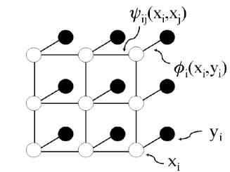
Fig. 1 depicts the graph that represents our pairwise MRF for computing the two-node beliefs. In the square lattice, $\psi_{ij}\left(x_{i},x_{j}\right)$ stands for the interaction potential that penalizes every dissimilar pair of neighboring labels, and $\phi\left(x_{i},y_{i}\right)=p\left(y_{i}|~{}x_{i}\right)$ represents the statistical dependency between the labels $x_{i}$ and the measurements $y_{i}$. For computing $b_{ij}\left(x_{i},x_{j}\right)$, $\phi\left(x_{i},y_{i}\right)$, is set to a constant value, making the result independent of the data values $y$.

We solve (28) by a line search type algorithm, ensuring that $\frac{\partial^{2}Q}{\partial^{2}\beta}\leq 0$, thus corresponding to a maximum of $Q$.

III-D A few Remarks about the Vector of Parametres $\phi$

In the previous section, we have considered that the class parameter vector $\phi$ is known and only the smoothness parameter $\beta$ is to be inferred. However, still using the beliefs computed by LBP, the vector $\phi$ could have been inferred simultaneously with $\beta$ by including in the $Q$ function the additive term (21) corresponding to the class densities. We would have obtained

$$Q(\phi;\phi_{t},\beta_{t}) = E[\log p(y|x)|y,\phi_{t},\beta_{t}]$$

$$= \sum_{i=1}^{N}\sum_{l=1}^{c}\log p(y_{i}|\phi^{l})p(x_{i}=l|y,\phi_{t},\beta_{t}),$$

where the probabilities $p(x_{i}=l|y,\phi_{t},\beta_{t})$ are given by the LPB method. The M-step would consist then in two decoupled maximizations; one with respect to $\beta$ and another with respect to $\phi$. This approach is, however, beyond the scope of this paper. Nevertheless, we present in Section V an unsupervised algorithm, which is suboptimal but faster than the LBP based EM algorithm aimed at the inference of both the parameters $\beta$ and $\phi$.

An alternative to the proposed EM scheme based on LPB is using Monte Carlo techniques to cope with the difficulty in computing the E-step and the partition function $Z$ [28], [29], [30]. Supported on the performance of the LBP, we believe, however, that the EM scheme based on LPB is, for the present problem, much more faster than the Monte Carlo based techniques.

IV Supervised Segmentation

In this section, we introduce two supervised algorithms aimed at the segmentation of sea SAR images. In both algorithms, the first step is the estimation of the class parameters used in the data model. This is done by asking the user to define representative regions of interest (ROI) in the image. Once the regions are defined, different approaches may be followed: if a Gamma mixture is assumed for the observed data, as in the case of SAR images, the EM class parameters estimation algorithm described in Appendix is applied to infer the class conditional densities. If we are segmenting small sub-scenes and the radar range spreading loss has been compensated in the underlying SAR images, one single Gamma function per class often provides a good modeling for the SAR intensities. In this case, a common ML Gamma estimator is used instead of the EM procedure. After this step, the data model is considered to be known and is used thereafter.

The pseudo-code for two supervised algorithms is presented in Algorithm 1 and Algorithm 2. Algorithm 1 is of generalized likelihood type [31] implementing an iterative labeling scheme with two steps being performed alternately: the $\beta$-Estimation and the segmentation. Algorithm 2 is a one-shot procedure that performs $\beta$-Estimation using the Loopy $\beta$-Estimation method described in Section III-C.

Algorithm 1 Supervised Segmentation Using LSF/CD $\beta$-Estimation

0:  Initial parameter $\hat{\beta}=\beta_{0}$ and estimated class parameters $\hat{\phi}$

1:  Compute $eLabel=E^{p}(x_{p})$ for every pixel $p$ using $\hat{\phi}$

2:  while $\left|\Delta\hat{\beta}\right|\leq\delta$ or nrIterations $<$ NrIterationsMax do

3:     Compute $\hat{x}=\alpha$-Expansion$(\hat{\beta},eLabel)$

4:     Compute $\hat{\beta}=\beta$-Estimation$(\hat{x},eLabel)$ {LSF or CD}.

5:  end while

6:  return  $\left(\hat{x},\hat{\beta}\right)$

Algorithm 2 Supervised Segmentation Using Loopy-$\beta$-Estimation

0:  estimated class parameters $\hat{\phi}$

1:  Compute $eLabel=E^{p}(x_{p})$ for every pixel $p$ using $\hat{\phi}$

2:  Compute $\hat{\beta}=\mbox{Loopy}$-$\beta$-Estimation($eLabel$)

3:  Compute $\hat{x}=\mbox{GraphCut}$-Segmentation$(\hat{\beta},eLabel)$

4:  return  $\left(\hat{x},\hat{\beta}\right)$

V Unsupervised Segmentation

The unsupervised method is an improvement of the supervised algorithms described in the previous sections. The main difference is that the data model is not considered to be known but is also iteratively estimated along with the smoothness parameter and the segmentation. The scheme needs a rough initialization of the data model parameters. We computed this initialization by fitting an EM Gamma mixture to the complete data.

As our EM algorithm automatically eliminates unnecessary modes, we start with an overestimate of $K$, the number of modes in the mixtures. In our experiments with real data, the maximum number of modes we got was four.

Then, different strategies are possible. In the experiments reported in the next section, when considering $c=2$ classes, we have assigned the mode with a lower mean value to one of the classes and the remaining modes to the other class.

In each iteration, we compute the ML estimate of the vector $\phi$ based on the previous segmentation, compute the new segmentation, and finally the new value of $\beta$. The algorithm may use any of the three $\beta-$parameter estimation methods and is applicable to an optional number of classes. The algorithm stops when both the parameter $\beta$ and the class parameters $\phi$ converge to stable values.

Algorithm 3 Unsupervised Segmentation

0:  arbitrary parameter $\hat{\beta}=\beta_{0}$, initial class parameters $\hat{\phi}=\phi_{0}$ (EM Gamma Mixture Estimation)

1:  Compute $eLabel_{0}$ = $E^{p}(x_{p})$ for every pixel $p$, using $\phi_{0}$

2:  Compute initial labeling $\hat{x}=x_{0}=\alpha$-Expansion$(\beta_{0},eLabel_{0})$

3:  for stop criterium is not met  do

4:     Compute $\hat{\phi}=$ ML-Estimation$(\hat{x})$

5:     Compute $eLabel=E^{p}(x_{p})$ for every pixel $p$, using $\hat{\phi}$

6:     Compute $\hat{x}=\alpha$-Expansion$(\hat{\beta},eLabel)$

7:     Compute $\hat{\beta}=\beta$-Estimation$(\hat{x},eLabel)$ {use LSF, CD or Loopy}.

8:  end for

9:  return  $\left(\hat{x},\hat{\beta},\hat{\phi}\right)$

VI Results

This section presents results of applying the proposed methodology to simulated and real SAR images, as well as some considerations regarding time complexity of the algorithms.

VI-A Simulations

We have performed simulations corresponding to Gamma data terms with two classes, and evaluated the overall accuracies of the obtained segmentations using Algorithms 1, 2 and 3. We also illustrate in detail the EM Gamma mixture estimation algorithm, by applying it to an example of simulated data.

VI-A1 Segmentation Results with Gamma Data Term

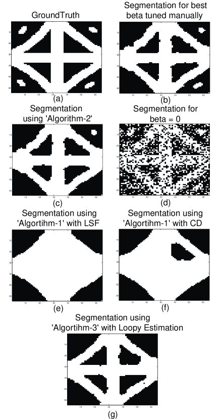
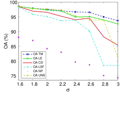
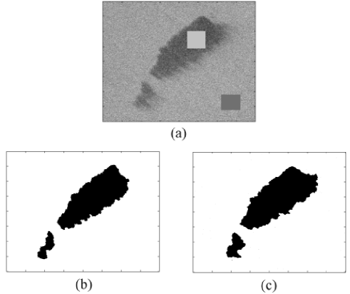
In order to compare the performance of the three proposed methods, we have tested Algorithms 1, 2 and 3 on simulated images generated by adding Gamma noise to ground-truth images containing two classes. We have used the ground-truth depicted in Fig. 2 (a) and added noise with Gamma distributions having mean values of five and nine. The parameters of the distributions were choosen in order to obtain increasing values of variance $\sigma^{2}$, corresponding to noisier images. We have then applied Algorithm 1,with LSF and CD methods, Algorithm 2, and Algorithm 3 with Loopy-$\beta$-Estimation. Furthermore, for comparison, the images were also segmented tuning the beta value manually and for the case that no prior is used ($\beta=0$). Fig. 2 shows the segmentations obtained for $\sigma=2.6$. As we can see from $\beta=0$ this is a hard problem, on which LSF and CD fails the inner structures, but Loopy-$\beta$-Estimation provides better results, both in the supervised as in the unsupervised method. This behavior is further confirmed by the rank in Fig. 3, which gives the OA obtained for images with different $\sigma$ values (corresponding to images with more noise) for the six different segmentation processes referred above.

Figure 2: Ground-truth and results of different segmentation processes for an image with Gamma noise having mean values of five and nine and with a $\sigma$ value $=2.6$. Notice the good performance of Algorithm 2 and Algorithm 3, implementing the Loopy-$\beta$-Estimation.

Figure 3: OA for images corrupted with Gamma noise with increasing $\sigma$ values: TM $\equiv$ for $\beta$ tuned manually; LE $\equiv$ Algorithm 2, using Loopy Estimation; LSF $\equiv$ Algorithm 1 using LSF; CD $\equiv$ Algorithm 1 using CD, NP $\equiv$ no prior and UNS $\equiv$ Algorithm 3 using Loopy Estimation.

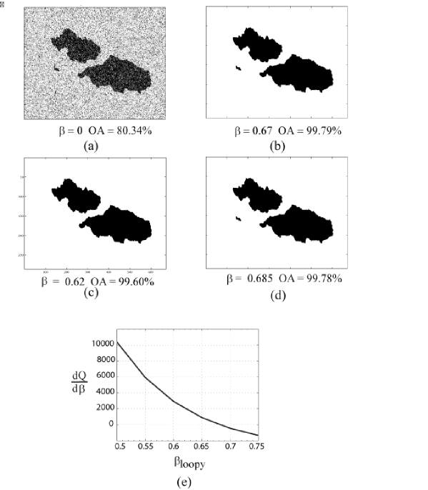
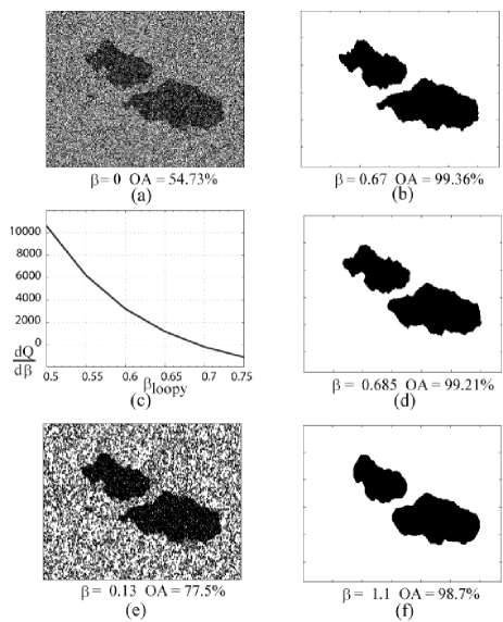
We have also tested the proposed algorithms in images generated by adding Gamma noise to a ground-truth similar to an oil patch (see Fig. 4). Two images, Image A and Image B, with the histograms depicted in Fig. 4, corresponding to different segmentation difficulty levels are segmented. The best segmentation possible in this framework, achieved by tuning the $\beta$ value manually, and the segmentation obtained with no prior information (setting $\beta=0$) are also displayed for comparison. Fig. 5 shows the results obtained for Image A and Fig. 6 the results obtained for Image B. For Image A, the segmented images using Algorithm 1, with CD and with LSF, are not shown, as they are almost equal to the image segmented with Algorithm 2. For Image B, Algorithm 3 has not provided good results and the segmentation is not displayed. The bad performance of Algorithm 3 in this case arises from the not so good initialisation of the class parameters, due to the complete overlapping from the oil and the water histogramms.

Figure 4: Gamma Model: (a) Ground-truth, (b) Histogram of Image A, (c) Histogram of Image B, (d) Image A, (e) Image B with superimposed delimiting line, for better visualization

Figure 5: Segmentation results for image A: (a) No prior information, (b) $\beta$ value tuned manually, (c) Segmentation using Algorithm 3 with Loopy-$\beta$-Estimation, (d) Segmentation using Algorithm 2 (Algorithm 1 provided the same results with only 0.1% difference in OA), (e) graph depicting the $\beta$ estimation in Algorithm 2.

Figure 6: Segmentation results for Image B: (a) No prior information, (b) $\beta$ value tuned manually, (c) graph depicting $\beta$ estimation using Algorithm 2, (d) Segmentation using Algorithm 2, (e) Segmentation using Algorithm 1 with LSF and (f) Segmentation using Algorithm 1 with CD.

VI-A2 EM Algorithm for Gamma Mixture

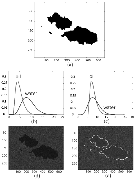
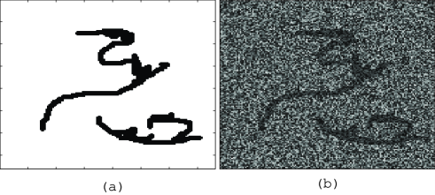
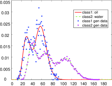
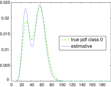
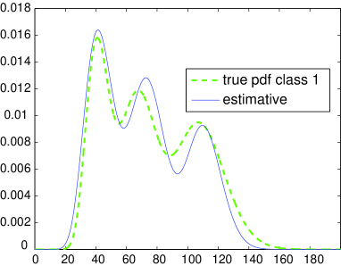
In this subsection we illustrate the behavior of the EM algorithm designed to infer Gamma mixtures. For details on the theoretical issues, we refer to the Appendix. In Fig. 7, we can see the ground-truth used for simulating the image and the generated image, according to the densities shown in Fig. 8. The two classes, oil and water have been modeled respectively by a mixture of two Gamma functions and a mixture of three Gamma functions. For this particular case, we have selected a ROI containing 178 pixels for representing the water and a ROI containing 142 pixels for representing the oil. After 20 iterations of the EM algorithm, we obtained the approximations for the probability distributions depicted in Fig. 9 and Fig. 10. The obtained results are quite reasonable for the small sample sizes used.

Figure 7: (a) Ground-truth used for simulating an oil spill. Black represents oil and white water; (b)Simulated SAR image

Figure 8: Probability functions used to generate the simulated image with superimposed histogram of generated data set. A three modes function for water and two modes function for oil was used.

Figure 9: True and estimated class densities for oil.

Figure 10: True and estimated class densities for water.

VI-B Real Images

We have tested the proposed methodology with three real SAR images for the special purpose of oil spill detection. For this type of application, an unsupervised algorithm is more indicated, and so we decided to apply Algorithm 3. Because Loopy Estimation has proven to be an effective method in the simulations, we have choosen Algorithm 3 with Loopy Estimation. Nevertheless, in order to have a comparision unsupervised approach versus supervised approach, we also applied Algorithm 2 to two of the images. In oil spill detection, the number of classes is typically set to $c=2$, although more classes can be considered if we are interested in distinguishing other phenomena occuring at the same time in the region of interest. The application of the algorithms is straightforward: the key idea, like in most state-of-the-art oil spill detection methods (see for example [16]), is to partition the image in tiles and run the algorithm separately for each part. This step is preceeded by the application of a landmask to the image, what can be done using external coastline information or by adopting some coastline self-extraction procedure. After the segmentation of each tile, a procedure for grouping patches detected on the tile borders should be carried on. Another possibility to increase segmentation coherency in the borders is to define overlapping tiles or to force continuity to some degree on the estimated class and/or smoothness parameters from one tile to the next. Nevertheless, at the moment we are not doing this and these are considered future possible improvements to our methodology. We segmented oil spills contained in three different scenes, described in the following subsections.

VI-B1 Segmentation of an ERS-1 sub-scene

We have segmented part of an ERS-1 image from the Sicily Channel, Italy, that has been acquired on the 30${}^{\textrm{th}}$ January of 1992. This image is referred in the ESA web pages regarding oil slicks http://earth.esa.int/ew/oil_slicks/ and contains three oil slicks, along with information regarding wind direction and intensity and existence of ships, ship wakes, natural oil films and currents.

Figure 11: ERS-1 image from the Sicily Channel, Italy, acquired on 30th January of 1992. The smaller and larger squares are sub-scenes that have been used respectively to estimate the wind direction and to apply our algorithm.

Figure 12: Closer look to the sub-scenes of the ERS-1 image. Part (a) is used for wind direction estimation; the estimated direction has been overlapped as a green arrow. Part (b) contains an oil spill. The coloured regions correspond to the ROI’s selected for class parameter estimation in the supervised algorithm

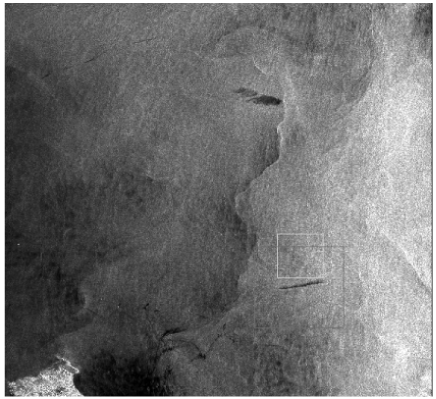
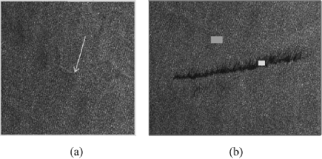
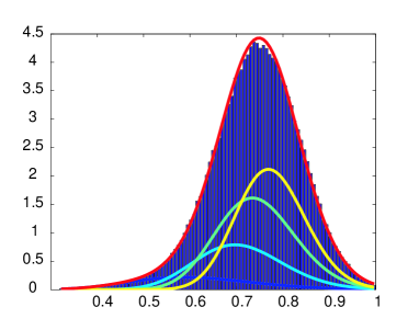
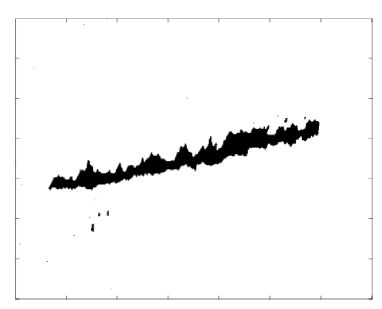
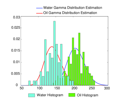
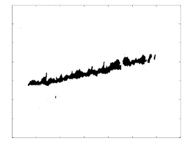
Fig. 11 provides a quicklook of the scene with two squares superimposed: the larger representing the part to be segmented and the smaller representing a part used for wind estiamtion. Fig. 12 provides zooms of the referred squares. By applying the Radon Transform to the smaller square, the estimated direction has been calculated and is depicted in the image. The direction was consistent with the measured value reported in the url site and is at the origin of the well-known ”feathering” effect that can be observed in this linear spill. We have computed the backscattering values of the image, by performing calibration using the ESA provided BEST software (http://earth.esa.int/services/best/) and then applied Algorithm-3 with Loopy-$\beta$-Estimation. The result of the Gamma mixture estimation, in the initialisation of the algorithm, is depicted in Fig. 13. After only three iterations, both the class parameters and the smoothness parameter have converged. A $\beta$ value equal to 1.4 was estimated. The segmentation is displayed in Fig. 14. We also applied Algorithm-2: we selected two ROI’s (160 pixels for water and 77 for oil) in the image (shown in Fig. 12) and computed ML Gamma Estimators for the two classes (see Fig. 15). We then applied the algorithm and obtained an estimated $\beta$ value equal to 1.44. The segmentation result is given in Fig. 16 and is similar to the result obtained with Algorithm-3.

Figure 13: Fitting of a mixture of Gammas to the data from the red square in the ERS-1 image.

Figure 14: Segmentation of ERS-1 subscene containing oil with $\beta=1.4$, estimated using Algorithm-3 with the Loopy-$\beta$-Estimation method.

Figure 15: Class Parameters Estimation for Algorithm-2.

Figure 16: Segmentation of ERS-1 subscene containing oil with $\beta=1.44$, estimated using Algorithm-2.

For comparison, we also provide the segmentation obtained with no prior (corresponding to $\beta=0$) in Fig. 17. In practice, the estimated value has proved to deliver a good segmentation. When lower $\beta$ values were used, the result was noisier and for higher $\beta$ values, the details of the spill disappeared.

Figure 17: Segmentation of ERS-1 subscene containing oil, with $\beta=0$.

VI-B2 Segmentation of an Envisat ASAR IM sub-scene

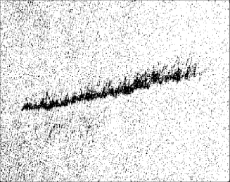
We have also applied Algorithm 3 to a fragment of an ASAR Image Mode image, acquired on 19 July 2004, in the ocean between Cyprus and Lebanon. The fragment contained an occurred oil spill of circa 10 km’s (centered on $\approx 33^{\circ}$N$,33^{\circ}$E$39$’) that was documented on the EC Oceanides project (a project in the framework of the Europe ’s Global Monitoring for Environment and Security initiative) database. After six iterations, we achieved convergence of the $\beta$ and $\theta$ values. The segmentation result is given in Fig. 18, corresponding to a estimated $\beta=1.83$. The unsupervised segmentation result is compared with the one provided by Algorithm-2, where the user provided ROI’s for water and for oil that were used to estimate the class parameters at the beginning of the process (see Fig. 18). In this case a $\beta=1.75$ was obtained.

Figure 18: (a) ASAR image fragment with coloured regions for class parameter estimation in Algorithm-2; (b) Segmentation result applying Algorithm-2; (c) Segmentation result applying Algorithm-3 with Loopy-$\beta$-Estimation.

VI-B3 Segmentation of an Envisat ASAR WSM sub-scene

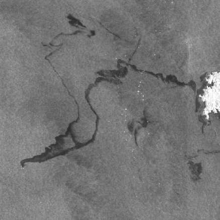
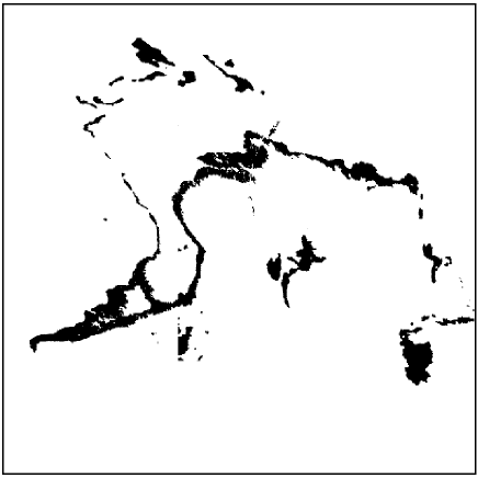
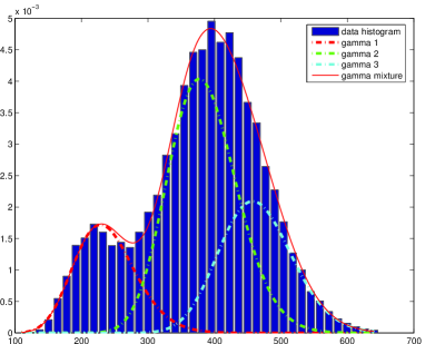
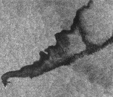
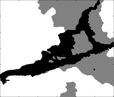
In order to demonstrate the viability of applying Algorithm 3 to a whole ASAR_WSM scene, we have run it over the very well known image of a confirmed oil spill, namely the Prestige case (see Fig. 19). This accident took place in November 2002, in Galicia (Spain), when a tanker carrying more than 20 million gallons (around 67,000 tons) of oil split in half off the northwest coast of Spain on 19 November 2002, threatening one of the worst environmental disasters in history. For segmenting the image, we have first partitioned it in tiles of 600x600 pixels each and then applied Algorithm-3 to each tile independently. No post-processing of the borders or “clean-up” operations (like for example morphological operations) have been carried out. Fig. 20 shows the segmented image, made up of the concatenation of the segmentation of the individual tiles. As we can see, the result can be considered in general very good, with only some discrepancies located on the tiles’ borders. For initialising the algorithm, the EM Gamma mixture estimation procedure was applied with four modes ($K=4$). In fact this number is enough to provide a good fitting of the intensity data of the SAR image. On the other hand, our EM algorithm allows us to start with a higher mode number, and decreases this number automatically. We depict the results of this fitting on one of the tiles, shown in Figure 23, by showing the histogram of the tile with the superimposed estimated Gamma mixture (see Fig. 21 (a)). As we have explained, the mode corresponding to the lower mean value is assigned to the oil class and the others to the water class, providing an initialisation to the class parameters. The estimations of these parameters are actualised along the algorithm and, after nine iterations, we obtain the distributions shown in Fig. 21 (b).

Figure 19: Display of the ASA WSM full resolution image of the Prestige accident occured in November 2002 in Galicia.

Figure 20: Display of the segmentation results of applying Algorithm 3 with Loopy-$\beta$-Estimation to the image displayed in Fig. 19.

Figure 21: Results of applying the EM Gamma mixture estimation procedure to the tile depicted in Figure 23: (a) Histogramm of the data values (normalised) with superimposed estimated Gamma mixture; (b) Distributions corresponding to the oil class (left) and water class (right) after nine iterations of Algorithm 3: Histogramm and superimposed fitting.

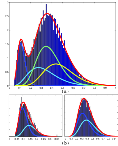
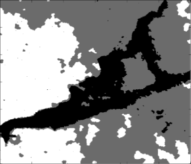
To fully demonstrate the possibilities of our algorithm, we again run it on the tile shown in Figure 23, but this time setting the number of classes to $c=3$. By doing so, we hope to be able to segment a third ambiguous zone, corresponding to intermediate radiometry levels and probably due to atmospheric conditions originating a front. In this case we choose to fitt a Gamma mixture of $c$ modes to the data for initialising the class parameters, as depicted in Fig. 22. With this initialisation, the first obtained segmentation using Algorithm 3 is displayed in Fig. 24, after only nine iterations, all parameters have already converged to the segmentation given in Fig. 25. When comparing this segmentation with the one provided by a state-of-the-art algorithm, namely by multiscale HMC model in [14], we consider to have obtained a very good result.

Figure 22: Histogramm of the data values (normalised) with superimposed estimated Gamma mixture when the number of classes is set to $c=3$

Figure 23: Display of one of the individual tiles in which the image in Figure 19 has been divided for segmentation.

Figure 24: Display of the initial segmentation result of applying Algorithm 3 with Loopy-$\beta$-Estimation and three classes to the tile depicted in Figure 23.

Figure 25: Display of the final segmentation result, after nine iterations, of applying Algorithm 3 with Loopy-$\beta$-Estimation and three classes to the bottom left tile of Fig. 17.

VI-B4 Time considerations

The proposed algorithms display, in practical cases, a computational complexity of $O(N)$, with N being the number of pixels in the image. In fact, the most time-consuming steps in the algorithms are the $\alpha$-Expansion and Graph-Cut segmentation routines. These use the max-flow code implementation referred in [32] that has complexity $O(n^{2.5})$ in the worst-case, however, in most situations is $O(N)$. Both Algorithm 1 and Algorithm 3 converge in few iterations and, as an example, for images of the dimension used in the first simulation (64x64) (see VI-A1), only a few seconds are needed to run the algorithms. For a 600x600 pixel tile, like those in the Prestige example in VI-B3, Algorithm 3 is taking $\approx$ 1 minute, but this time performance could be improved by a more efficient implementation of our procedure, namely by improving the implementation of the Loopy-$\beta$-Estimation and by migrating our matlab code fully to C-code.

VII Conclusions

The results of applying the proposed methodology to simulated images with Gamma data models and to real SAR data are promising. The developed EM Gamma mixture estimation algorithm, when incorporated into the proposed segmentation algorithms, has proved to be an efficient tool for data modeling in SAR intensity images.

With the supervised algorithms, high OA accuracies have been achieved even for simulated images with high levels of noise. In general the Bayesian approach has resulted in an OA increase in the segmentation process between $10$ and $15\%$, when compared to the segmentation using no prior information. Hereby, Algorithm 1 with LSF and Algorithm 1 with CD methods provided similar results, with a performance close to that obtained by setting the $\beta$ value manually. On the other hand, the LSF estimation procedure seems to become less reliable for noisier images. When compared to Algorithm 2, using Loopy-$\beta$-Estimation, we see that this last method allways provides equal or better results, outcoming Algorithm 1. Another advantage of Algorithm 2 is that it is usually faster than Algorithm 1, being a one-shot process. Both algorithms, by introducing prior information into the segmentation process, increase the OA significantly. As a conclusion, Algorithm 2 should be preferred to Algorithm 1, when using a supervised method for oceanic sar images segmentation.

Algorithm 3, totally unsupervised, has been conceived as an improvement to Algorithm 1 and 2. When testing it on simulated data the obtained results were very good, although slightly worst than the supervised ones, as expected. In general, after a few iterations, the class and smoothness parameters converge to stable and meaningful values. By applying Algorithm 3 to real images containing documented oil spills, the segmentation has been considered successfull. We could segment both linear and patch type oil spills. Furthermore, the applicability of the method to segment whole scenes, as well as to segment more than two classes, has also been demonstrated in a well known image from the Prestige accident. As a conclusion, we believe the presented methods are suitable to be used for segmenting oceanic SAR images. In particular for oil spill detection, Algorithm 3 seems to be a suitable method.

Based on observations that oil spills in the ocean are often dragged by the wind and align more or less perpendicular to its direction, an interesting future issue is the incorporation of wind information into our segmentation algorithms. By adopting anisotropic MRF in the prior, we intend to reflect this directional dependency of the clique potentials. In the practice, the smoothness parameter $\beta$ is no longer considered to be a constant value but is clique-dependent according to the wind direction and/or velocity. For estimating the wind profile from the SAR data, state-of-the-art algorithms are used. We have run promissing simulations, are currently testing this extension on real data, and expect to obtain interesting results on a near future.

Fitting a Mixture of Gamma Densities

As stated in the main text of this work, when segmenting real SAR images, the adopted data model for each class is a finite Gamma mixture. For completely defining the data model for each class (for lightness of the notation we have dropped the class index), we need to estimate $2K$ Gamma parameters, $\theta=(\theta_{1},\dots,\theta_{K})$, with $\theta_{s}=(a_{s},\lambda_{s})$, and $K$ a priori probabilities $\alpha=(\alpha_{1},\dots,\alpha_{K}))$. We infer $\phi=(\alpha,\theta)$ by computing its ML estimate from a training set. The ML estimate is computed via an EM algorithm [26]. Fitting a Gamma mixture is addressed in [33]. However, the authors consider $N$-look SAR images meaning that the underlying random variables are the average of $N$ independent and identically distributed exponential random variables, thus, having a Gamma density but with just one parameter free; if the mean is $\mu$, then the variance is given by $\mu^{2}/N$. We estimate both the mean and the variance for each Gamma distribution in the mixture, rendering the algorithm more adaptable to real measurements.

The key point in the EM technique is the introduction of the so called missing data $z$, such that $p\left(y|\phi\right)=\int p\left(y,z|\phi\right)dz$ and $p\left(y,z|\phi\right)$ is easier to manipulate than $p\left(y|\phi\right)$. In the particular case of a mixture of densities, we will use as missing data a random variable, $z_{i}$, per site, with distribution $p(z_{i}=s)=\alpha_{s}$. It is interpretable as the probability of the $s-th$ Gamma mode is selected at pixel $i$. The EM algorithm alternates between two steps: the E-step computes the conditional expectation of the logarithm of the complete a posteriori probability function, with respect to the missing variables, based on the actual parameter value. The M-step updates the values of the parameters, by maximizing the expression obtained in the E-step with respect to each parameter on turn, i.e.,

E-step $$: Q\left(\phi;\phi^{t}\right)=E\left\{\log{p\left(y,z|\phi\right)|y,\phi^{t}}\right\}$$ (29)

M-step $$: \phi^{t+1}=\arg\max_{\phi}Q\left(\phi;\phi^{t}\right)$$ (30)

Denoting

$$w_{si}^{t}=P\left(z_{i}=s|y_{i},\phi^{t}\right)\\$$ (31)

and taking into account that $\sum\alpha_{s}$ = 1, then $\phi^{t+1}$ can be found among the stationary points of the Lagrangean

$${\cal L}(\phi)=\sum_{i=1}^{N}\sum_{s=1}^{K}\left(L_{si}(\theta_{s},\alpha_{s})\,w_{si}^{t}\right)+\lambda\left(\sum_{s=1}^{K}\alpha_{s}-1\right),\\$$ (32)

with

$$L_{si}(\theta_{s},\alpha_{s}) = \log{\left(\lambda_{s}^{a_{s}}\right)}-\log{\left[\Gamma\left(a_{s}\right)\right]}$$ (33)

$$+\log{\left(y_{i}^{a_{s}-1}\right)}-\lambda_{s}y_{i}+\log{\left(\alpha_{s}\right)},$$

where $\lambda$ denotes a Lagrange multiplier. The expression for $w_{si}^{t}$ (see [34]) is given by

$$w_{si}^{t}=\frac{\alpha_{s}^{t}p(y_{i}|\theta_{s}^{t})}{\sum_{r=1}^{K}\alpha_{r}^{t}p(y_{i}|~{}\theta_{r}^{t})}.\\$$ (34)

In the M-step, after differentiating ${\cal L}$ in order to the unknown parameters and setting the derivatives to zero, we obtain a closed solution for the updating of the a priori probabilities $\alpha_{i}$’s, but numerical iteration is needed for determining parameters $a_{i}$’s and $\lambda_{i}$’s of the Gamma densities. Expression (35) gives the update expression for $\alpha_{i}$’s.

$$\alpha_{s}^{t+1}=\frac{1}{N}\sum_{i=1}^{N}w_{si}^{t}.\\$$ (35)

Equation (36) and (37) give the update expressions for the parameters $\lambda_{i}$’s and $a_{i}$’s.

$$\lambda_{s}^{t+1}=\frac{a_{s}^{t}\sum_{i=1}^{N}w_{si}^{t}}{\sum_{i=1}^{N}y_{i}w_{si}^{t}},\\$$ (36)

$$a_{s}^{t+1}=\Psi^{-1}\left[\frac{\log{\left(\lambda_{s}^{t}\right)}\sum_{i=1}^{N}w_{si}^{t}+\sum_{i=1}^{N}\log{(y_{i})}w_{si}^{t}}{\sum_{i=1}^{N}w_{si}^{t}}\right],\\$$ (37)

where

$$\Psi\left(a_{s}\right)=\frac{\Gamma^{\prime}\left(a_{s}\right)}{\Gamma\left(a_{s}\right)},\\$$ (38)

is the psi function. We refer to the Appendix B of [35] for a very fast Newton procedure to compute the inverse of the psi$(\cdot)$ function. Expressions (36) and (37) are iteratively recomputed until convergence is obtained, starting from initial values computed from the observed data y. The initial parameter values are calculated in such a way, that the initial probability function is a sum of equidistant Gammas that span the most representative data range. The EM scheme converges in a few tens of iterations.

Acknowledments

We thank V. Kolmogorov for the max-flow code made available at http://www.cs.cornell.edu/People/vnk/software.html, used in the Graph-Cut and $\alpha$-Expansion segmentation techniques and S. Kumar for the Loopy Belief Propagation code used for computing the two-node beliefs in the Loopy-$\beta$-Estimation EM algorithm described in Section III-C.

References

- [1] C. R. Jackson and J. R. Apel, Synthetic Aperture Radar Marine User’s Manual, Commerce Dept., NOAA, 2005.
- [2] S. Y. Wu and A. K. Liu, “Towards an automated ocean feature detection, extraction and classification scheme for SAR imagery,” International Journal Remote Sensing, vol. 24, no. 5, pp. 935–951, 2003.
- [3] C. Brekke and A. Solberg, “Oil spill detection by satellite remote sensing,” Remote Sensing of Environment, vol. 95, pp. 1–13, 2005.
- [4] G. Mercier and F. Girard-Ardhuin, “Partially supervised oil-slick detection by SAR imagery using kernel expansion,” IEEE Transactions on Geoscience and Remote Sensing, vol. 44, no. 10, pp. 2839–2846, February 2006.
- [5] S. Pelizzari and José M. B. Dias, “Bayesian adaptive oil spill segmentation of SAR images via graph cuts,” in Proceedings of the SeaSAR, 2006.
- [6] S. Pelizzari and José M. B. Dias, “Bayesian oil spill segmentation of SAR images via graph cuts,” in Proceedings of the IbPRIA, 2007, vol. 2, pp. 637–644.
- [7] S. Pelizzari and José M. B. Dias, “Oil spill segmentation of SAR images via graph cuts,” in Proceedings of the IGARSS, 2007, pp. 1318 – 1321.
- [8] T. Silva J. B. Dias and J. Leit ao, “Adaptive restoration of speckled SAR images using a compound random Markov field,” in Proceedings of ICIP, 1998, vol. 2, pp. 79–83.
- [9] R. Garello Y. Delignon and A. Hillion, “Statistical modelling of ocean SAR images,” IEEE Proc.-Radar, Sonar Navigation, vol. 144, no. 6, pp. 348–354, December 1997.
- [10] S.Z.Li, Markov Random Field Modeling in Computer Vision, Springer-Verlag, Tokyo, 1995.
- [11] J. Yedidia, W. Freeman, and Y. Weiss, “Understanding belief propagation and and its generalizations,” in Proceedings of International Joint Conference on Artificial Intelligence, 2001.
- [12] V. Kolmogorov and R. Zabih, “What energy functions can be minimized via graph cuts?,” IEEE Transactions on Pattern Analysis and Machine Intelligence, vol. 26, no. 2, pp. 147–159, February 2004.
- [13] Y. Boykov, O. Veksler, and R. Zabih, “Fast approximate energy minimization via graph cuts,” IEEE Transactions on Pattern Analysis and Machine Intelligence, vol. 23, no. 11, pp. 1222–1239, 2001.
- [14] S. Derrode and G. Mercier, “Unsupervised multiscale oil slick segmentation from SAR images using a vector hmc model,” Pattern Recognition, vol. 40, pp. 1135–1147, 2007.
- [15] A. Gambardella M. Migliaccio and M. Tranfaglia, “SAR polarimetry to observe oil spills,” IEEE Transactions on Geoscience and Remote Sensing, vol. 45, no. 2, pp. 506–511, February 2007.
- [16] C. Brekke A. Solberg and P.Husøy, “Oil spill detection in Radarsat and envisat SAR images,” IEEE Transactions on Geoscience and Remote Sensing, vol. 45, no. 3, 2007.
- [17] G. Mercierb V.P. Onanac J. Mvogo Ngonoc P.L. Frisond J.P. Rudantd T. Kanaa, E. Tonyea and R. Garellob, “Detection of oil slick signatures in SAR images by fusion of hysteresis thresholding responses,” in Proceedings of IGARSS, 2003, vol. 4, pp. 2750–2752.
- [18] P. Réfrégier F. Galland and O. Germain, “Synthetic aperture radar oil spill segmentation by stochastic complexity minimization,” IEEE Geoscience and Remote Sensing Letters, vol. 1, no. 4, 2004.
- [19] S. Geman and D. Geman, “Stochastic relaxation, Gibbs distributions and the Bayesian restoration of images,” IEEE Trans. Patt. Analysis and Mach. Intel., vol. PAMI-6, no. 6, pp. 721–741, 1984.
- [20] S. YuE M. Berthod, Z. Kato and J. Zerubia, “Bayesian image classification using Markov random fields,” Image and Vision Computing, vol. 14, pp. 285–295, 1996.
- [21] H. Derin P. Kelly and K.D.Hartt, “Adaptive segmentation of speckled images using a hierarchical random field model,” IEEE Transactions on Acoustics, Speech, and Signal Processing, vol. 36, no. 10, pp. 1628–1641, 1988.
- [22] G. Vézina H. Derin, P. Kelly and S.G.Labitt, “Modeling and segmentation of speckled images using complex data,” IEEE Transactions on Geoscience and Remote Sensing, vol. 28, no. 1, pp. 76–87, 1990.
- [23] P.C.Smits and S.G.Dellepiane, “Synthetic aperture radar image segmentation by a detail preserving Markov random field approach,” IEEE Transactions on Geoscience and Remote Sensing, vol. 35, no. 4, pp. 844–857, 1997.
- [24] C. Jakowatz, D. Wahl, P. Eichel, D. Ghiglia, and P. Thompson, Spotlight-Mode Synthetic Aperture Radar: A Signal Processing Approach, Kluwer, Norwell, MA, 1996.
- [25] N. Jonhnson and S. Kotz, Distribution in Statistics: Continuous Univarite Distributions, vol. 1, Wiley, New York, 1996.
- [26] N. Laird A. Dempster and D. Rubin, “Maximum likelihood estimation from incomplete data via the EM algorithm,” Journal of the Royal Statistical Society B, vol. 39, pp. 1–38, 1977.
- [27] S. Kumar, J. August, and M. Hebert, “Discontinuity preserving surface reconstruction through global optimization,” in EMMCVPR, LNCS, 2005, vol. 3757, pp. 153–168.
- [28] M. Ibáñez and A. Simó, “Parametric estimation in Markov random fiels image modeling with imperfect observations. a comparative study,” vol. 24, pp. 2377–2389, 2003.
- [29] L. Younes, “Parametric inference for imperfectly observed Gibbsian fields and some comments on Chalmond’s EM Gibbsian algorithm,” Probability Theory and Related Fields, vol. 82, pp. 625–645, 1989.
- [30] L. Younes, “Parametric inference for imperfectly observed Gibbsian fields and some comments on Chalmond’s EM Gibbsian algorithm,” in Proc. Stochastic Models, Statistical Methods and Algorithms in Image Analysis, P. Barone and A. Frigessi, Eds., Berlin, Germany, 1991, vol. 47 of Lecture Notes in Statistics, pp. 240–258, Springer.
- [31] S. Lakshamanan and H. Derin, “Simultaneous parameter estimation and segmentation of gibbd random fields using simulated annealing,” IEEE Trans. Patt. Analysis and Mach. Intel., vol. 11, pp. 793–813, 1989.
- [32] Y. Boykov and V. Kolmogorov, “An experimental comparison of min-cut/max-flow algorithms for energy minimization in vision,” IEEE Transactions on Pattern Analysis and Machine Intelligence, vol. 26, no. 9, pp. 1124–1137, 2004.
- [33] S. Wang Q. Jiang A. E. Zaart, D. Ziou and G. B. Bénié, “SAR images segmentation using mixture of Gamma distributions,” in Proceedings of Vision Interface, 1999.
- [34] G. McLachlanand and D. Peel, Finite Mixture Models, John Wiley and Sons, New York, 2000.
- [35] José M. Nascimento, Unsupervised Hyperspectral Unmixing, Ph.D. thesis, Instituto Superior Tecnico, 2006.