Observation of universal behaviour of ultracold quantum critical gases

Abstract

Quantum critical matter has already been studied in many systems, including cold atomic gases. We report the observation of a universal behaviour of ultracold quantum critical Bose gases in a one-dimensional optical lattice. In the quantum critical region above the Berezinskii-Kosterlitz-Thouless transition, the relative phase fluctuations between neighboring subcondensates and spatial phase fluctuations of quasi-2D subcondensates coexist. We study the density probability distribution function when both these two phase fluctuations are considered. A universal exponential density probability distribution is demonstrated experimentally, which agrees well with a simple theoretical model by considering these two phase fluctuations.

The nature of quantum criticality Hertz ; Sachdev ; Cole driven by quantum fluctuations is still a great puzzle, despite of the remarkable advances in heavy-fermion metals and rare-earth-based intermetallic compounds, etc Gegen . New understanding of quantum criticality is widely believed to be a key to resolving open questions in metal-insulator transitions Imada , high temperature superconductivity HS and novel material design, etc. Cold atoms in optical lattices provide a unique chance to not only simulate other strongly correlated systems RMP-Bloch , but also study some models unaccessible in solid state systems, particularly for the Bose-Hubbard model Fisher ; Jaksch ; Bloch . Despite of its complexity, a strongly correlated system in quantum critical regime is expected to exhibit a universal behaviour described by a certain physical quantity.

Here we report the observation of universal behaviour for ultracold quantum critical Bose gases in a one-dimensional optical lattice. Density probability distributions of the released gases are measured for different depths of the lattice potential. It was found that the density probability follows a simple exponential law when the Bose gases reach the quantum critical region above the Berezinskii-Kosterlitz-Thouless (BKT) transition BKTtheory1 ; BKTtheory2 ; Pol ; BKTexp . This universal behaviour can be well understood in terms of our theoretical model considering both the relative phase fluctuations of quasi-2D subcondensates and spatial phase fluctuations of individual subcondensates above the BKT transition. The method of density probability distribution should provide a unique tool for identifying certain quantum phases of optical lattice systems.

Ultracold Bose atoms in 1D, 2D and 3D optical lattices are widely studied by the Bose-Hubbard model Fisher . At zero temperature, there is a continuous quantum phase transition from superfluid (SF) to Mott insulator (MI). Because of the strongly correlated quantum behaviour, the quantum critical point (QCP) at absolute zero temperature distorts strongly the structure of the phase diagram at finite temperatures, leading to the emergence of an unconventional ‘V-shaped’ quantum critical region Sachdev ; Ho ; Cap ; Kato ; Chin ; Haz (Fig. 1). In analogy with a black hole, the crossover to quantum critical gas involves crossing a ‘material event horizon’, which implies strongly that the quantum critical gas has a simple and universal behaviour Cole .

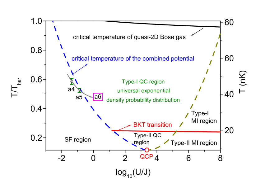
Figure 1: Finite temperature phase diagram of ultracold Bose gases in a one-dimensional optical lattice. $U$ and $J$ represent the strengths of the on-site repulsion and of the nearest neighbor hopping in the Bose-Hubbard model, respectively. By increasing the strength of an optical lattice, $U/J$ can be increased by several orders of magnitude. The existence of the quantum critical point (QCP) at zero temperature leads to a ‘V-shaped’ quantum critical (QC) region. Apart from the ordinary SF-QC-MI transition, the BKT transition for quasi-2D subcondensates can also occur at sufficiently low temperatures. In the QC region above the BKT transition (Type-I QC region), there exists a universal behaviour in the density probability distribution. All the phase boundary lines, except for the dashed line between QC and MI regions, are calculated with a total atom number of $1.1\times 10^{5}$ and trap parameters used in the experiment. $T_{har}$ is the critical temperature for the purely harmonic trap in absence of the optical lattice. The gray line displays a phase transition path from SF to Type-I QC region. Data points of (a4)-(a6) along the gray line are obtained from the corresponding absorption images in Fig. 2

In the commonly used 3D optical lattice systems, the atoms in a lattice site are strongly confined in all directions, with a mean occupation number per lattice site of about $1\sim 3$ Bloch . Thus the spatial phase fluctuations for the atoms in a single lattice site can be omitted, and the relevant theoretical calculations based on the Bose-Hubbard model Fisher ; Jaksch and Wannier function Kohn can give quantitative descriptions of almost all experimental phenomenaRMP-Bloch . In contrast, for ultracold Bose atoms in a 1D optical lattice, unique characteristics may arise due to the following two reasons:

(1) Quasi-2D Bose gas: In an experiment of 1D optical lattice system as ours, there can be hundreds of atoms in a lattice site. The Bose gas in a lattice site becomes quasi-two-dimensional (quasi-2D) Pedri ; Burger ; Had , if the local trapping frequency $\widetilde{\omega}_{z}$ of a lattice site in the lattice direction satisfies the condition $\hbar\widetilde{\omega}_{z}>>k_{B}T$ Pethick .

(2) BKT transition: For such a quasi-2D Bose gas, the critical temperature in the occupied lattice site is given by $T_{2D}\approx\hbar\omega_{\perp}\left(N_{l}\zeta\left(2\right)\right)^{1/2}/k_{B}$, with $N_{l}$ being the atomic number in a lattice site. Well below $T_{2D}$, the whole system becomes a chain of subcondensates. If there is no correlation between the subcondensates in different lattice sites, a quasi-2D gas undergoes a BKT transition at $T_{BKT}=T_{2D}/4$ BKTtheory1 ; BKTtheory2 . Beyond this critical value of $T_{BKT}$, it is favorable to create vortices in quasi-2D subcondensates, and the unbinding of bound vortices will lead to strong spatial phase fluctuations within each subcondensate.

Since the BKT transition is crucial to revealing the property of cold atoms in a 1D optical lattice, its critical temperature is also plotted in the phase diagram (red line in Fig. 1). The BKT transition line divides the QC region into two parts (Type I and Type II). Our experiments focus on the transition from SF region to QC region above the BKT transition.

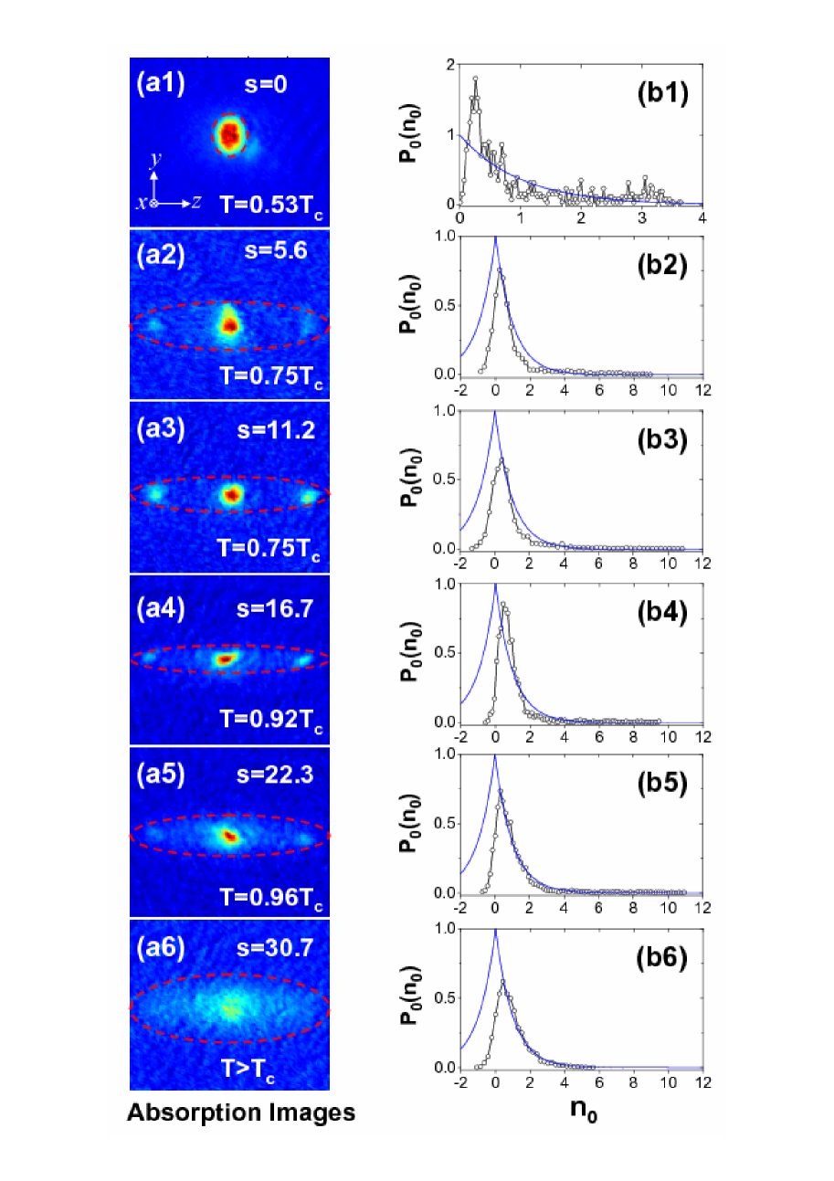
Figure 2: Density probability distribution for different lattice depths. (a1)-(a6) in the left column are absorption images showing the density distribution of the released atomic clouds. The field of view is $0.9\times 0.9$ mm², and the pixel size is $\Delta^{2}=9.0\times 9.0$ $\mathrm{\mu m}^{2}$. $T_{c}$ denotes the critical temperature of the atomic gas in the combined trap. For moderate $s$, the interference fringes are prominent. Further increasing $s$, however, we see complete disappearance of the interference fringes (a6). This is due to the crossover from SF to QC region as $s$ is increased. (b1)-(b6) in the right column are the corresponding density probability distributions. Open circles are the data points calculated from the density distributions of the images in the left column. The blue solid curves give the exponential density probability distribution $P_{0}^{e}$ defined in text. When $s$ becomes large enough, the data points agree well with the exponential curve (see b5 and b6), which shows clearly a universal behaviour in the QC region above the BKT transition.

The experiments started with pure ⁸⁷Rb condensates confined in a magnetic trap with axial and transverse trapping frequencies of $\left\{\omega_{\bot},\omega_{z}\right\}=2\pi\left\{83.7,7.6\right\}$ Hz. The 1D optical lattice was formed by a retroreflected laser beam of $\lambda=800\,$nm along the axis ($z$ direction) of the condensate. This laser beam was ramped up to a given intensity over a time of $50$ ms, yielding a lattice potential $V_{opt}=sE_{R}\sin^{2}\left(2\pi z/\lambda\right)$, with $E_{R}$ being the recoil energy of an atom absorbing one lattice photon. After a holding time of $10$ ms, we suddenly switched off the combined potential and allowed the cold atomic cloud to expand freely for a time of $30$ ms.

The expanded atomic gases were probed using the conventional absorption imaging technique. Since the probe beam is applied along $x$ direction, what an absorption image records is the two-dimensional ($y-z$) column density profile of the atomic cloud. We denote by $N_{1}^{ph}\left(y,z\right)$ and $N_{2}^{ph}\left(y,z\right)$ the number of photons detected in the pixel at position $\left(y,z\right)$ with and without the atomic cloud, respectively. Then the density distribution is written as $n_{2D}\left(y,z\right)=\ln\left[N_{2}^{ph}\left(y,z\right)/N_{1}^{ph}\left(y,z\right)\right]\Delta^{2}/\sigma_{e}$, with $\sigma_{e}$ being the absorption cross section of a single atom and $\Delta$ the pixel size.

The left column of Fig. 2 ((a1)-(a6)) displays the density distributions for different lattice depths $s$. The temperatures of the system were inferred from the condensate fractions as described in the Appendix. From the top three images ((a1)-(a3)), we see an increasing of the side peaks in the interference patterns as $s$ is increased. Further increasing $s$, we find the interference fringes become blurred and disappear eventually (see (a4)-(a6)), similar to the experimental observation in Ref. Orzel . The gradual disappearance of the interference fringes can be partially explained by the increasing of the random relative phase Orzel during the SF-QC transition. In Figs. 2(a5)-(a6), except for the density fluctuations along $z$ direction associated with the random relative phase between different subcondensates, we also see significant density fluctuations along $y$ direction. The simultaneous existence of density fluctuations in these two directions is further demonstrated in Fig. 3 (c) and (d) for a typical case of $s=30.7$. These experimental results suggest that in the QC region above the BKT transition, both the random relative phases and spatial phase fluctuations play important roles in the expanded density distribution.

Figure 3: Density fluctuations of the released atomic clouds. (a)-(d) are one-dimensional cuts through the corresponding images. For $s=30.7$, the density distribution is highly fluctuated along both the horizontal ($z$) and vertical ($y$) directions.

To qualitatively analyze the density fluctuations, we consider the following density probability distribution

$$P\left(n\right)=\frac{S\left(n-\delta n/2\right)-S\left(n+\delta n/2\right)}{\delta n\cdot S_{\mathrm{total}}}\,,$$ (1)

where $\delta n$ is the width of a density interval, $S_{\mathrm{total}}$ is the total area of the region occupied by the atomic gas, while $S\left(n\right)$ is the area of the region where the density larger than $n$. The averaged density is $n_{s}=1/S_{\mathrm{total}}$. For convenience, we define a dimensionless density as $n_{0}=n/n_{s}$. The dimensionless density probability distribution is then $P_{0}\left(n_{0}\right)=n_{s}P\left(n\right)$.

The right column of Fig. 2 displays $P_{0}\left(n_{0}\right)$ calculated from the corresponding density distribution. In each image, the pixel region chosen for the calculation of $P_{0}\left(n_{0}\right)$ is that occupied by the cold atoms, as enclosed by the red dashed ellipse. In all our calculations of $P_{0}\left(n_{0}\right)$, $\delta n_{0}$ is just the horizontal spacing of discrete data points. Due to the optical noise, $P_{0}\left(n_{0}\right)$ can be nonzero even for negative $n_{0}$. This can be understood from the atomic density formula based on the absorption imaging signal. Assuming $n_{0b}$ is the minimum negative density for nonzero $P_{0}\left(n_{0}\right)$, optical noise concentrates in the region of $n_{0b}<n_{0}<\left|n_{0b}\right|$ in each $P_{0}\left(n_{0}\right)$ plot. Thus, $n_{0}>\left|n_{0b}\right|$ gives the effective region where the optical noise is negligible and $P_{0}\left(n_{0}\right)$ reflects the true density probability distribution.

The blue solid lines in Fig. 2(b1)-(b6) represent the following exponential density probability distribution

$$P_{0}^{e}=e^{-\left|n_{0}\right|}.$$ (2)

It is obvious that, with increased $s$ (and hence $U/J$), $P_{0}\left(n_{0}\right)$ has a tendency to $P_{0}^{e}$. In Fig. 2(b6), we see that $P_{0}\left(n_{0}\right)$ agrees well with $P_{0}^{e}$ in the whole effective region. Despite of the extremely complex many-body state in the QC region above the BKT transition, our results show a simple universal behaviour.

We have numerically simulated our experiments to explain the exponential density probability distribution. When a released gas has experienced a free expansion over a time of $t$, the 2D density distribution is given by

$$n_{2D}\left(y,z,t\right)=\int dx\left|\sum_{k}\sqrt{N_{k}}e^{i\left(\phi_{k\perp}\left(x,y,t\right)+\phi_{k}^{s}\left(z,t\right)\right)}\varphi_{k\perp}\left(x,y,t\right)\varphi_{kz}\left(z,t\right)\right|^{2}+n_{2D}^{opt}\left(x,y\right).$$ (3)

Here $\varphi_{k\perp}\left(x,y,t\right)\varphi_{kz}\left(z,t\right)$ is the wave packet of the expanded subcondensate initially in the $k$th lattice site, with $|\varphi_{k\perp}\left(x,y,t\right)|^{2}$ being the Thomas-Fermi density distribution in transverse ($x$-$y$) directions, and $|\varphi_{kz}\left(z,t\right)|^{2}$ the Gaussian density distribution along $z$ direction. Two classes of phase fluctuations enter the expression. $\phi_{k\perp}\left(x,y,t\right)$ represents the spatial phase fluctuations in transverse directions, while $\phi_{k}^{s}\left(z,t\right)$ comprises the relative phase fluctuations between different subcondensates. $N_{k}$ denotes the atomic number of the $k$th subcondensate. The term $n_{2D}^{opt}$ is added to account for the optical noise. In numerical calculations, it was simulated with the realistic optical noise distribution in the region having no atoms.

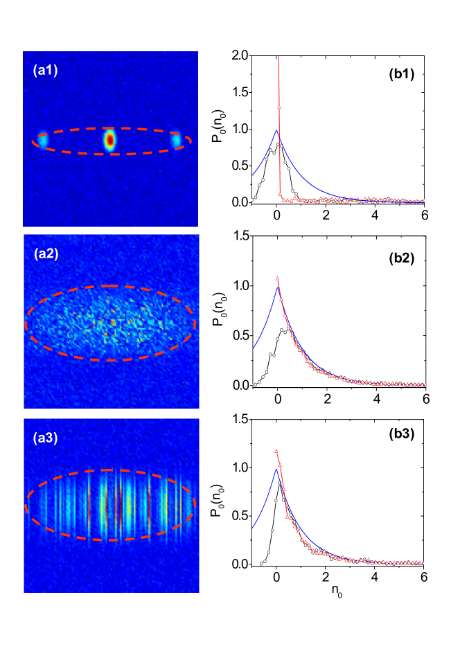
Figure 4: Theoretical simulation. Left column: simulated density distributions based on Eq. (3). (a1), (a2) and (a3) are three typical cases in which an atomic gas initially stays in SF, Type-I QC and Type-II QC regions, respectively. In (a1), $s=11.2$, $\delta\phi_{k\perp}=0.2\pi$. In (a2), $s=30.7$, both $\phi_{k}^{s}$ and $\phi_{k\perp}$ are completely random. In (a3), $s=30.7$, $\phi_{k\perp}=0$, but $\phi_{k}^{s}$ is completely random. Each of the color map has a size of $0.9\times 0.9$ mm². Right column: Black lines are the density probability distribution calculated from the corresponding density distributions in the left column. Red lines are obtained under the same conditions except that the optical noise is not included. The exponential density probability distribution (blue lines) is also plotted for comparison. The data in (b2) clearly shows an exponential density probability distribution in the QC region above the BKT transition.

Figs. 4(a1) and (b1) give the simulated density distribution and density probability distribution for an atomic gas initially in the combined trap with $s=11.2$. Spatial phase fluctuations ($\phi_{k\perp}$) have been assumed to be zero. Figs. 4(a2) and (b2) display similar calculations for $s=30.7$, but with completely random phases $\phi_{k\perp}$ and $\phi_{k}^{s}$. The theoretical results in Figs. 4(b2) match the exponential density probability distribution, in agreement with our experimental results. The coexistence of two random phases of $\phi_{k\perp}$ and $\phi_{k}^{s}$ makes the system similar to the situation of the interference of randomly scattered waves Sheng , where exponential distribution is also found. More general analytical derivations for Eq. (3) and the exponential density probability distribution are given in the Appendix. Figs. 4(a3) and (b3) give the simulation of $s=30.7$ for a cold atomic gas in the QC region below the BKT transition. Accordingly, $\phi_{k\perp}$ is assumed to be zero, while there exists a completely random relative phase in $\phi_{k}^{s}$. No exponential density probability distribution is found in this simulation. In addition, we do not notice regular interference fringes either. Note that in Ref. Had , the QC region far below the BKT transition was studied experimentally. However, because there are only about $30$ subcondensates, high-contrast interference fringes were still observed. Since our calculation is based on the experimental parameters in this work, the total number of subcondensates is much higher (up to $250$).

To further explain the experimental phenomena, we stress that there are two completely different situations in determining the BKT transition temperature for cold atoms in 1D optical lattices.

(1) BKT transition in QC and MI regions: In these two regions, the quasi-2D Bose gases in different lattice sites can be regarded as independent subcondensates as far as the BKT transition is concerned. By minimizing the free energy $F=E-TS$ ($E$ and $S$ are the energy and entropy of the Bose gas in a lattice site when vortices are considered), one can get the BKT transition temperature $T_{BKT}=T_{2D}/4$ Pethick . In the MI region above the BKT transition, Eq. (3) can be used to simulate the density distribution by including a completely random relative phase in $\phi_{k}^{s}$ Had , if the averaged particle number per lattice site is much larger than $1$. Thus, in the MI region above the BKT transition, one still expects the exponential density probability distribution for a large number of more than one hundred independent subcondensates.

(2) BKT transition in SF region: In the SF region, although the Bose gases in the lattice sites become quasi-2D, they are highly correlated. For a series of $M$ highly correlated quasi-2D Bose gases, the free energy becomes $F=ME-TS$. If there are vortices in the quasi-2D subcondensates, vortices in different lattice sites are highly correlated in spatial locations. Thus, $S$ can be approximated as the entropy of a single subcondensate. Then the BKT transition temperature becomes $T_{BKT}^{M}=MT_{BKT}$. Since $M>100$, we see that $T_{BKT}^{M}>>T_{2D}$. This means that the temperatures of quasi-2D condensates are always much lower than the BKT transition temperature. For the situation of $s=11.2$ in our experiment, based on the estimation of the particle number fluctuations $\delta N_{k}$ Jav and the relation of $\delta\phi_{k}^{s}\sim 2\pi/\delta N_{k}$ Orzel , we deduced a phase fluctuation of $\delta\phi_{k}^{s}\approx 0.2\pi<<2\pi$, which shows strong correlation between different lattice sites. As shown in Fig. 3(b), there are no noticeable density fluctuations along $y$ direction, which confirms that the initially confined gas is well below the BKT transition even though $T$ is already beyond $T_{BKT}$.

We should also emphasize that, in the QC region above the BKT transition, the system cannot be regarded as a classical thermal cloud although the temperature is higher than the critical temperature $T_{c}$. A classical thermal cloud features density fluctuations as $\delta^{2}n\approx n$. In contrast, the exponential density probability distribution corresponds to much larger density fluctuations of $\delta^{2}n\approx n^{2}$ XiongWu . This exponential density probability distribution physically originates from the superposition of quantum sates with a completely random phase, while the universal behaviour lies in that the distribution is always exponential for completely random superposition of quantum state XiongWu . The present work supports the long-standing belief that the quantum states in the QC region are strongly correlated, and there should be a simple universal behaviour, once appropriate physical quantity is found Sachdev ; Cole ; Gegen .

Appendix

Bose-Hubbard model. The combined potential of a one-dimensional (1D) optical lattice and a harmonic trap is given by

$$V=\frac{1}{2}m\omega_{\perp}^{2}\left(x^{2}+y^{2}\right)+\frac{1}{2}m\omega_{z}^{2}z^{2}+sE_{R}\sin^{2}\left(\frac{2\pi z}{\lambda}\right).$$ (4a)

Here $$E_{R} \lambda z \widetilde{\omega}_{z}\simeq 2\sqrt{s}E_{R}/\hbar$$ is the recoil energy of an atom absorbing one lattice photon with wavelength . For an atom in a lattice site, it experiences an effective harmonic potential along direction with angular frequency .

Bose-condensed gases in 1D, 2D and 3D optical lattices are widely studied by the following Bose-Hubbard model FisherS

$$\widehat{H}=-\sum\limits_{\left\langle ij\right\rangle}J\widehat{a}_{i}^{{\dagger}}\widehat{a}_{j}+\frac{U}{2}\sum\limits_{i}\widehat{n}_{i}\left(\widehat{n}_{i}-1\right)+\sum\limits_{i}\left(\varepsilon_{i}-\mu\right)\widehat{n}_{i}.$$ (4b)

Here $\widehat{n}_{i}=\widehat{a}_{i}^{{\dagger}}\widehat{a}_{i}$ is the number operator at the $i$th site, with $\widehat{a}_{i}^{{\dagger}}$ ($\widehat{a}_{i})$ being the boson creation (annihilation) operator. $U$ and $J$ represent the strengths of the on-site repulsion and of the nearest neighbor hopping, respectively. $\varepsilon_{i}$ describes an energy offset due to the harmonic trap, and $\mu$ is the chemical potential. The phase diagram given by Fig. 1 in the text is calculated with the above combined potential and Bose-Hubbard model.

Universal exponential density probability distribution. The many-body quantum state in the QC region can be written as in a general way

$$\left|\Psi_{qcr}\right\rangle=\sum_{\left\{\Sigma N_{k}=N\right\}}C\left(N_{1},\cdot\cdot\cdot,N_{2k_{M}+1}\right)\prod_{k}\frac{1}{\sqrt{N_{k}!}}\left(\widehat{a}_{k}^{{\dagger}}\right)^{N_{k}}\left|0\right\rangle.$$ (4c)

Here $N_{k}$ denotes the atomic number in the $k$th lattice site. The total atomic number is then $N=\Sigma_{k=-k_{M}}^{k=k_{M}}N_{k}$, with $2k_{M}+1$ being the total number of occupied lattice sites. For strongly correlated quantum gases in the QC region, the function $C\left(N_{1},\cdot\cdot\cdot,N_{2k_{M}+1}\right)$ is extremely complex, and no analytical expression exists. After switching off the combined potential, the density distribution is then

$$n\left(x,y,z,t\right)=\left\langle\Psi_{qcr}\left(t\right)\right|\widehat{\Psi}^{{\dagger}}\widehat{\Psi}\left|\Psi_{qcr}\left(t\right)\right\rangle.$$ (4d)

Assuming that the initial wave function in the $k$th lattice site is $\varphi_{k}\left(x,y,z,t=0\right)=\varphi_{k\perp}\left(x,y,t=0\right)\varphi_{kz}\left(z,t=0\right)$, for long-time evolution so that the expanded subcondensates have sufficient overlapping with each other, we have

$$n\left(x,y,z,t\right)\approx\left|\sum_{k}\sqrt{N_{k}}e^{i\phi_{k}^{s}\left(z,t\right)}\varphi_{k\perp}\left(x,y,t\right)\right|^{2}\left|\varphi_{0z}\left(z,t\right)\right|^{2}.$$ (4e)

This formula holds in the QC region, because there are non-negligible particle number fluctuations in each lattice site. Here $\phi_{k}^{s}\left(z,t\right)=\phi_{k}^{r}+\phi_{k}^{0}$, with $\phi_{k}^{r}$ being a completely random relative phase in the QC region. $\phi_{k}^{0}=m\left(z-k\lambda/2\right)^{2}/2\hbar t$ can be obtained directly from the free expansion along $z$ direction. Without the random phase $\phi_{k}^{r}$, the phase $\phi_{k}^{0}$ will lead to clear interference fringes along $z$ direction with a period of $4\pi\hbar t/m\lambda$ PedriS . It is understood that there would be no interference fringes along $z$ direction if $\phi_{k}^{s}$ is a completely random relative phase, as shown in Figs. 2(a5)-(a6) in the text.

In the QC region above the BKT transition, there are two sorts of random phases: (i) the completely random phase $\phi_{k}^{s}\left(z,t\right)$ in the QC region; (ii) the spatially relevant random phase $\phi_{k\perp}\left(x,y,t\right)$ above the BKT transition. In this region, the density distribution can be further written as

$$n\left(x,y,z,t\right) \approx \left|\sum_{k}\sqrt{N_{k}}e^{i\phi_{k\perp}\left(x,y,t\right)}e^{i\phi_{k}^{s}\left(z,t\right)}\right|^{2}$$ (4f)

$$\left|\varphi_{0\perp}\left(x,y,t\right)\varphi_{0z}\left(z,t\right)\right|^{2}.$$

Here $\phi_{k\perp}\left(x,y,t\right)$ physically originates from the spatial phase fluctuations of quasi-2D Bose gas above the BKT transition.

The density distribution recorded by a CCD is a 2D density distribution $n_{2D}\left(y,z,t\right)=\int dxn\left(x,y,z,t\right)$. By assuming that $\left|\varphi_{0\perp}\left(x,y,t\right)\varphi_{0z}\left(z,t\right)\right|^{2}$ is locally constant (i.e. the local density approximation), after integrating out the $x$ variable, we have

$$n_{2D}\left(y,z,t\right) \approx \left|\frac{1}{\sqrt{2k_{M}+1}}\sum_{k}\alpha_{k}\left(y,z,t\right)e^{i\beta_{k}\left(y,z,t\right)}\right|^{2}$$ (4g)

$$n_{2D}^{0}\left(y,z,t\right),$$

with $n_{2D}^{0}\left(y,z,t\right)=\int dx\left|\sqrt{N}\varphi_{0\perp}\left(x,y,t\right)\varphi_{0z}\left(z,t\right)\right|^{2}$. $\alpha_{k}\left(y,z,t\right)$ and $\beta_{k}\left(y,z,t\right)$ are statistically independent random real function, because they originates from two different random phases $\phi_{k}^{s}\left(z,t\right)$ and $\phi_{k\perp}\left(x,y,t\right)$. $\beta_{k}\left(y,z,t\right)$ distributes uniformly between $-\pi$ and $\pi$. The normalization condition requests $\left\langle\alpha_{k}^{2}\right\rangle=1$.

Based on the central limit theorem Feller , we get the following exponential density probability distribution

$$P\left(n_{2D}\left(x,y,t\right)\right)=\frac{e^{-n_{2D}\left(x,y,t\right)/n_{2D}^{0}\left(x,y,t\right)}}{n_{2D}^{0}\left(x,y,t\right)}.$$ (4h)

For uniform $n_{2D}^{0}$, it is straightforward to get Eq. (2) in the text. For nonuniform $n_{2D}^{0}$, with the local density approximation, Eq. (2) in the text is a very good approximation obtained from Eq. (4h).

In Figs. 2(b5)-(b6) in the text, we see that the density probability distribution agrees well with the exponential density probability distribution. However, because the system temperature is slightly smaller than the critical temperature for Fig. 2(b5) ($s=22.3$), we expect Fig. 2(b6) agrees better with the exponential density probability distribution. Here we give the semilog plot of the density probability distribution for $s=22.3$ and $s=30.7$, respectively. We do find that the situation of $s=30.7$ agrees better with the exponential density probability distribution.

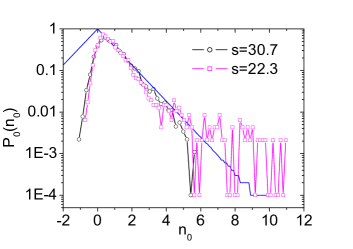
Figure 5: Semilog plot of the density probability distribution for $s=22.3$ and $s=30.7$. The blue line gives the exponential density probability distribution.

System temperature. In our experiment, the total atomic number can be accurately measured. The atomic numbers of Figs. 2(a4)-(a6) in the text are $1.10\times 10^{5}$, $1.19\times 10^{5}$ and $1.13\times 10^{5}$, respectively. To drive the system into the deeper region of superfluidity, we have to further lower the temperature of an atomic sample before loading it to the lattice. This is implemented by kicking more atoms out of the magnetic trap during the evaporative cooling stage. Specifically, for Figs. 2(a2) and (a3) in the text, the atomic numbers are reduced by about a factor of two compared with Figs. 2(a4)-(a6) in the text.

However, the measurement of the system temperature is hampered by the lack of accurate thermometry in optical lattices. Actually, the ratio $T/T_{c}$ is a more important quantity than $T$ in characterizing the transition from superfluid to quantum critical regions. Therefore, the inaccuracy of system temperature does not affect the physics of the present work, as long as $T/T_{c}$ can be somehow determined with a satisfying accuracy.

As predicted in Ref. Duan and demonstrated in a recent experiment Phillips , the appearance of superfluid in an inhomogeneous lattice is associated with a bimodal structure in the density profile. The condensate fraction $N_{0}/N$ can be obtained by fits to the bimodal distribution. As we have known, $N_{0}/N$ shows a temperature dependence having a characteristic shape as

$$N_{0}/N=1-(T/T_{c})^{\alpha}.$$ (4i)

Apparently, $T/T_{c}$ can be directly determined if the parameter $\alpha$ is known. Blakie et al. Tc-Blakie had performed numerical calculations of the critical temperature as well as the condensate fraction, for a combined trap similar to that in our work. Their results show that $\alpha$ is close to $3$ at a moderate lattice depth, but it may drop slightly with increasing lattice depth. Nevertheless, at a high depth level, the condensate fraction is usually very small, and, as a result, the value of $T/T_{c}$ derived from Eq. (4i) becomes insensitive to the potential errors of $\alpha$. Therefore, we just set $\alpha=3$ in the calculation of $T/T_{c}$, which seems to be a reasonable assumption.

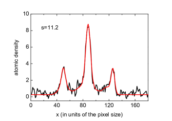
Figure 6: A bimodal fit to the interference pattern in Fig. 2(a3) in the text. The total atom number is measured as $N\simeq 5.9\times 10^{4}$, and the atomic cloud was released from the combined trap with a lattice strength of $s=11.2$. Black line, the measured atomic density which is obtained by integrating over each column of pixels. Red line, a fitting curve including six Gaussian peaks, where the three narrow peaks at the upper part are attributed to superfluid. The condensate fraction is $N_{0}/N\approx 0.58$, corresponding to $T/T_{c}\approx 0.75$.

For each absorption image, we first obtain the atomic density along the $z$ dimension by integrating pixels in each column. The narrow peaks riding over broad ones are regarded as the condensate parts. We then fit both the broad and the narrow peaks using Gaussian profiles, so as to get the condensate fraction. Apparently, this method works only when $T<T_{c}$. In Fig. 2(a6) in the text, the interference peaks vanish completely, indicating that $T>T_{c}$. In this case, we are unable to extract the quantity $T/T_{c}$ any more with this method. The universal exponential density probability distribution found in this work also implies that the accurate measurement of system temperature in the QC region above BKT transition is difficult.

References

- (1) M. P. A. Fisher, P. B. Weichman, G. Grinstein, D. S. Fisher, Phys. Rev. B 40, 546 (1989).
- (2) P. Pedri et al., Phys. Rev. Lett. 87, 220401 (2001).
- (3) G. D. Lin, W. Zhang, L. M. Duan, Phys. Rev. A 77, 043626 (2008).
- (4) I. B. Spielman, W. D., Phillips, J. V. Porto, Phys. Rev. Lett. 100, 120402 (2008).
- (5) P. B. Blakie, W. X. Wang, Phys. Rev. A 76, 053620 (2007).
- (6) W. Feller, An Introduction to Probability Theory and its Applications Vol. 1 (John Wiley & Sons, New York, 1957).