Magnetic Non-Potentiality of Solar Active Regions and Peak X-Ray Flux of the Associated Flares

Abstract

Predicting the severity of the solar eruptive phenomena like flares and Coronal Mass Ejections (CMEs) remains a great challenge despite concerted efforts for several decades. The advent of high quality vector magnetograms obtained from Hinode (SOT/SP) has increased the possibility of meeting this challenge. In particular, the Spatially Averaged Signed Shear Angle (SASSA) seems to be an unique parameter to quantify the non-potentiality of the active regions. We demonstrate the usefulness of SASSA for predicting the flare severity. For this purpose we present case studies of the evolution of magnetic non-potentiality using 115 vector magnetograms of four active regions namely ARs NOAA 10930, 10960, 10961 and 10963 during December 08$-$15, 2006, June 03$-$10, 2007, June 28$-$July 5, 2007 and July 10$-$17, 2007 respectively. The NOAA ARs 10930 and 10960 were very active and produced X and M class flares respectively, along with many smaller X-ray flares. On the other hand, the NOAA ARs 10961 and 10963 were relatively less active and produced only very small (mostly A and B-class) flares. For this study we have used a large number of high resolution vector magnetograms obtained from Hinode (SOT/SP). The analysis shows that the peak X-ray flux of the most intense solar flare emanating from the active regions depends on the magnitude of the SASSA at the time of the flare. This finding of the existence of a lower limit of SASSA for a given class of X-ray flare will be very useful for space weather forecasting. We have also studied another non-potentiality parameter called mean weighted shear angle (MWSA) of the vector magnetograms along with SASSA. We find that the MWSA does not show such distinction as the SASSA for upper limits of GOES X-Ray flux of solar flares, however both the quantities show similar trends during the evolution of all active regions studied.

1 Introduction

Many magnetic parameters e.g., twist, shear, energy etc. computed for complex active regions have been examined with a view to predict the severity of solar eruptive phenomenon like flare and Coronal Mass Ejections (CMEs). Although such studies have been carried out for several decades, the progress remains slow. Here we study two of these parameters i.e., magnetic non-potentiality inferred from the spatially averaged signed shear angle (SASSA) and mean weighted shear angle (MWSA) of sunspots.

Magnetic shear at polarity inversion lines were studied earlier to look for flare related changes (e.g., Hagyard et al., 1984; Hagyard et al., 1990; Ambastha et al., 1993; Hagyard et al., 1999). The magnetic energy change following few flares has been estimated by Schrijver et al. (2008); Jing et al. (2010). Jing et al. (2010) found that the magnitudes of free magnetic energy were different for the flare-active and the flare-quiet regions, but the temporal variation of free magnetic energy did not show any clear and consistent pre-flare pattern. A study of the evolution of global alpha ($\alpha_{g}$) for one highly eruptive and one quiet active region has been performed by Tiwari (2009). But no correlation between $\alpha_{g}$ and the GOES X-Ray flux was found. Sudol & Harvey (2005) found changes in the line of sight magnetic field associated with flares. The unsigned flux of NOAA AR 10930 has been studied recently by Abramenko et al. (2008). Figure 2 of Abramenko et al. (2008) shows that the unsigned net flux of NOAA AR 10930 does not show any relationship with the peak GOES X-ray flux.

Despite many such attempts, the severity of flares has not been successfully predicted. In this paper, we make an effort to determine an upper limit of the peak X-ray flux of solar flares emanating from the active regions as a function of the magnitude of the SASSA and the MWSA. These parameters, viz., SASSA and MWSA give quantitative measure of the non-potentiality present in an active region at the observed height. More details about the SASSA and the MWSA are given in Section 2.

Many researchers have used the force-free parameter $\alpha$ as a measure of the magnetic twist of the sunspots. Many forms of global $\alpha$ have been proposed and studied such as: $\alpha_{best}$ (Pevtsov et al., 1995), $\alpha_{av}$ (Hagino & Sakurai, 2004), $\alpha_{g}$ (Tiwari et al., 2009a; Tiwari et al., 2009b; Tiwari, 2009) etc. The force-free parameter $\alpha$ actually gives twice the degree of twist per unit axial length along the axis of the flux rope (see Appendix A of Tiwari et al. (2009a)). Thus, $\alpha$ provides the gradient of twist at a certain observational height and not the actual twist of an active region. The sign of the global $\alpha$ ($\alpha_{g}$) and the SASSA are found similar but the magnitudes are not correlated (Tiwari et al., 2009b). Recently, $\alpha_{g}$ has been studied for the time series of two active regions NOAA AR 10930 and 10961 by Tiwari (2009) as mentioned earlier. The global alpha does not show any clear indication for predicting the severity of the X-ray flares. The reason could be due to the non-validity of the linear force-free assumption for such complex ARs. The local and global $\alpha$ values of several active regions were studied by Hahn et al. (2005) and Nandy et al. (2003); Nandy (2008). They found that the global $\alpha$ ($\alpha_{best}$) was not important for the flare activity. However, they noticed a decrease in the variance of spatial $\alpha$ distribution after the flare.

To explore the utility of SASSA as a predictor of flare severity, we have studied the evolution of SASSA in a time series of vector magnetograms of two highly flare productive sunspots i.e., NOAA ARs 10930 and 10960 and also two less flare productive sunspot i.e., NOAA ARs 10961 and 10963. The AR 10930 has been the most active sunspot observed by Hinode (SOT/SP). Three major X-class flares i.e., X6.5, X3.4 and X1.5 were observed by Hinode (SOT/SP) on 06, 13 and 14 December, 2006 respectively. Many C and B-class flares were also associated with the same sunspot. Similarly NOAA AR 10960 was also highly flare productive and produced four M-class flares. On the other hand NOAA ARs 10961 and 10963 were relatively less flare productive.

The main purpose of this study is to find the lower limit of the non potentiality parameters, if any, for a given class of X-Ray flare.

In the following section (Section 2), we briefly describe the magnetic parameters SASSA and MWSA. In Section 3, we give details of the data sets used. Section 4 illustrates the analysis and results obtained. Finally, in Section 5 we discuss the results and present our conclusions.

2 The Magnetic Non-Potential Parameters Used in This Study

2.1 Spatially Averaged Signed Shear Angle (SASSA)

Signed shear angle (SSA) represents the deviation of observed transverse vectors from the potential transverse vectors with positive or negative sign. It has the similar sign as the photospheric chirality of the sunspots (Tiwari, 2009; Tiwari et al., 2009b). The SSA is computed from the following formula:

$$SSA=\tan^{-1}(\frac{B_{yo}B_{xp}-B_{yp}B_{xo}}{B_{xo}B_{xp}+B_{yo}B_{yp}})$$ (1)

where $B_{xo},B_{yo}$ and $B_{xp},B_{yp}$ are observed and potential transverse components of sunspot magnetic fields respectively.

A spatially averaged value of SSA (SASSA) is taken to quantify the global non-potentiality of the whole sunspot. This parameter gives the non-potentiality of a sunspot irrespective of the force-free nature (Tiwari et al., 2009b) and shape of the sunspot (Venkatakrishnan & Tiwari, 2009). Thus, SASSA is a very important magnetic parameter to quantify the non-potentiality of any active region.

Apart from measuring the non-potentiality, SASSA also retains the sign of chirality of the active region magnetic field, unlike other shear parameters such as MWSA. This property of sign seems to be crucial in obtaining the proper measure of global non-potentiality, as will be explained later in the paper.

2.2 Mean Weighted Shear Angle (MWSA)

The mean weighted shear angle was introduced by Wang (1992) to quantitatively study the changes in magnetic structure and the build-up of the magnetic shear. The mean weighted shear angle is given as

$$MWSA=\frac{\sum|B_{t}|~{}\theta}{\sum|B_{t}|}$$ (2)

where $B_{t}$ is the measured transverse field strength and $\theta$ is the difference between the observed and potential azimuths. The potential fields have been computed by taking the longitudinal field as boundary. The method used in computing the potential field is as per Sakurai (1989).

The reason for calculating weighted mean instead of a simple average of shear angle is that the MWSA filters the weak field area. The stronger fields play more important role in determining the field structure and can be measured more accurately. We should note here that the MWSA will weight more on the high transverse field regions like penumbral fields, a fact that will be shown later in the paper to explain the relatively lower success of MWSA as a flare intensity predictor.

3 Data Sets Used

We have used the series of vector magnetograms of two eruptive ARs NOAA 10930 and 10960 and two less-eruptive ARs NOAA 10961 and 10963 obtained from the Solar Optical Telescope/Spectro-polarimeter (SOT/SP: Tsuneta et al. (2008); Suematsu et al. (2008); Ichimoto et al. (2008); Shimizu et al. (2008)) onboard Hinode (Kosugi et al., 2007).

The Hinode (SOT/SP) data have been calibrated by the standard “SP_PREP” routine developed by B. Lites and available in the Solar-Soft package. The prepared polarization spectra have been inverted to obtain vector magnetic field components using an Unno-Rachkowsky (Unno, 1956; Rachkowsky, 1967) inversion under the assumption of Milne-Eddington (ME) atmosphere (Landolfi & Landi Degl’Innocenti, 1982; Skumanich & Lites, 1987). We use the “STOKESFIT” inversion code which is available in the Solar-Soft package and was developed by T. R. Metcalf. The latest version of the inversion code is used which returns the true field strengths along with the filling factor.

There is an inherent 180^∘ ambiguity in the azimuth determination due to the insensitivity of the Zeeman effect to the sense of orientation of the transverse magnetic fields. Numerous techniques have been developed and applied to resolve this problem (for details see Metcalf et al., 2006; Leka et al., 2009), but a complete resolution is not expected from the physics of the Zeeman effect. The chirality of chromospheric and coronal structures can be used as guides to complement the other methods. The 180^∘ azimuthal ambiguity in our data sets have been removed by using the acute angle method (Harvey, 1969; Sakurai et al., 1985; Cuperman et al., 1992). This method of ambiguity resolution works very well for magnetic shear angles that are less than 90 degrees. Less than one percent pixels of any vector magnetogram studied has shear $\sim 90$ degrees. Therefore, we expect that the acute angle method works well in all our cases. Most of the data sets used have a spatial sampling of $\sim 0.3$ arcsec/pixel. A few data sets are observed in “Normal Mode” of SOT with a spatial sampling of $\sim 0.16$ arcsec/pixel.

The noise in the data has been minimized in the similar way as was done in Tiwari (2009); Tiwari et al. (2009b) and Venkatakrishnan & Tiwari (2009, 2010). The method is as follows: the pixels having transverse $(B_{t})$ and longitudinal magnetic field $(B_{z})$ values greater than a certain level are only analyzed. To decide this critical threshold, a quiet Sun region is selected for each active region and the 1$\sigma$ deviation in the three vector field components $B_{x}$, $B_{y}$ and $B_{z}$ are evaluated separately. The resultant 1$\sigma$ deviation in $B_{x}$ and $B_{y}$ is then taken as the noise level for transverse field components. Only those pixels with longitudinal and transverse fields simultaneously greater than twice the above mentioned noise levels are analyzed.

To minimize the projection effects, the magnetograms are transformed to the heliographic coordinates wherever they are more than 10 degrees away from the disk-center (Venkatakrishnan et al., 1988; Venkatakrishnan & Gary, 1989).

The information about different classes of X-ray flares are collected from the web sites http://www.solarmonitor.org/index.php and http://www.spaceweather.com/. We have also used the GOES X-Ray data.

4 Data Analysis and Results

Figure 1 shows GOES 12 X-Ray plots (in the wavelength range 1.0$-$8.0 Å) of different X-Ray flares observed during the disk passage of NOAA ARs 10930, 10960, 10961 and 10963 respectively. We see that the GOES X-ray peaks show high activity with two X-class flares and several C-class flares during 08$-$15 December, 2006 in NOAA AR 10930 (Figure 1(a)). High activity is also seen with 4 M-class and several C-class flares during 03$-$10 June, 2007 through the disk passage of NOAA AR 10960 (Figure 1(b)). The GOES X-ray light curves show lesser activity with very small B and A class flares during June 28$-$July 05, 2007 in NOAA AR 10961 (Figure 1(c)). Figure 1(d) also presents a weak activity with some C-class flares in the beginning but mostly B and A-class flares in later evolution stages of NOAA AR 10963 during 10$-$18 July, 2007.

A large number of vector magnetograms of eruptive NOAA ARs 10930 (36) and 10960 (21) have been analyzed. Also, 28 and 30 vector magnetograms of lesser eruptive NOAA ARs 10961 and 10963 respectively, are analyzed to study the evolution of these sunspot magnetic fields. One longitudinal image with the transverse vectors of each active region has been shown in the Figure 2. The red and blue contours represent the positive and negative fields of $\pm 1000,\pm 1500,\pm 3000$ Gauss.

4.1 Temporal Evolution of SASSA and MWSA

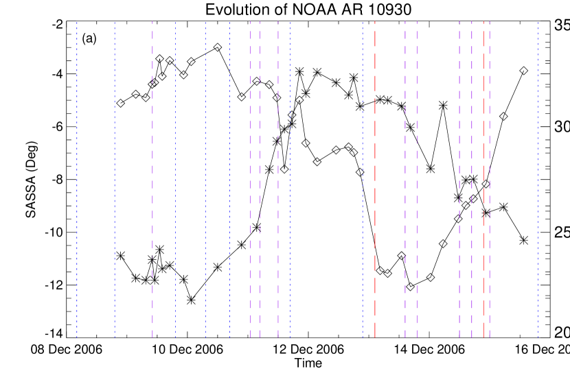
Figure 3: Evolution of SASSA and MWSA in NOAA ARs 10930 and 10960 is shown. The boxes and stars represent the SASSA and MWSA respectively. (a): The red big dashed vertical lines represent timings of two X-class flares. Purple colored smaller dashed lines show the timings of C-class flares and blue dotted lines represent the timings of the B-class flares. (b): The orange colored dash-dotted lines show the timings of the M-class flares. The dashed purple and dotted blue lines again show the timings of C and B-class flares as above.

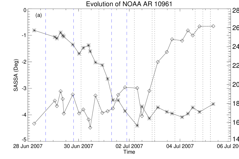
Figure 4: Evolution of SASSA in NOAA AR 10961 and NOAA AR 10963 shown. Both are relatively quiet regions. The boxes and stars represent the SASSA and MWSA respectively. (a): The blue colored dashed vertical lines represent the timings of the B-class X-ray flares and black dotted lines represent the timings of A-class flares. (b): The purple colored dashed lines show timings of C-class flares. The blue colored dashes and black dots represent timings of B and A-class flares respectively.

Figures 3 and 4 show the plots of SASSA and MWSA in highly active regions NOAA ARs 10930 and 10960 and relatively quiet NOAA ARs 10961 and 10963 respectively. The diamonds and stars represent the SASSA and MWSA respectively. The dotted/dashed vertical lines show the time and class of flares associated with these active regions. The lines with red colored big dashes in Figure 3(a) represent the timings of X-class flares. The orange colored dash-dotted lines in Figure 3(b) show the timings of M-class flares. The lines with purple colored small dashes in all figures represent the timings of C-class flares. The blue colored dotted lines in Figures 3(a) and 3(b) represent the timings of B-class flares. The black colored dotted lines in Figures 4(a) and 4(b) represent the timings of A-class flares whereas blue colored dashed lines in these figures represent the timings of B-class flares.

4.1.1 Evolution of SASSA and MWSA in NOAA AR 10930

From the plots of SASSA in Figure 3(a), it can clearly be noticed that any X-class flare happened only when the SASSA was greater than $8$ degrees. If the SASSA is greater than $4$ degree, then C-class flares also occurred. If the SASSA is less than $4$ degrees, only B-class flares happened. It should be noted that the sign of SASSA with magnitudes is given in the Figures only to express the sense of chirality of non-potentiality. Similarly, the MWSA was greater than 26 and 22 degrees for X and C-class flares respectively. B-class flares occurred if the MWSA was greater than 21 degrees.

We can notice that both the non-potentiality parameters show similar trend during the evolution period of the active region. However, the threshold values of MWSA for C and B-class flares are very close.

4.1.2 Evolution of SASSA and MWSA in NOAA AR 10960

Figure 3(b) shows that the M-class flares took place when SASSA exceeded 6 degrees. The M-class flares did not occur whenever SASSA was less than 6 degrees. One interesting behavior during the evolution of this active region can be noticed is the chirality inversion. The SASSA in the beginning is highly negative and three M-class flares took place. The SASSA started decreasing allowing only 3 C-class flares and became positive by building up non-potentiality again. As SASSA became more than 4 degrees, C-class flares again started taking place. After 7 C-class flares, one M-class flare happened when SASSA exceeded 6 degrees. Even in this peculiar evolution of the active region, the SASSA maintained its upper limits for different classes of X-ray flares as observed in the NOAA AR 10930. Thus we see a symmetrical behavior of the threshold values, independent of the sign of SASSA.

The MWSA shows an almost similar behavior as the SASSA. MWSA was high in the beginning, starts decreasing after some flares and again builds up showing a similar trend as SASSA. It can be noticed however that for C-class flares, MWSA goes very small up to 11 degrees and could not maintain its upper limit as decided in the case of NOAA AR 10930. The MWSA values observed for M-class flares are seen to be more than 22 degrees which mixes up with that of the C-class flares observed in NOAA AR 10930. Thus, the threshold values of MWSA seem to be specific to the active region and thus seem to be of dubious utility for flare intensity prediction.

4.1.3 Evolution of SASSA and MWSA in NOAA AR 10961

The NOAA AR 10961 is the quietest active region out of the four studied. Only B and A-class flares occurred during the disk passage of this active region as can be seen in Figure 4(a). From Figure 4(a), one can see that the B-class flares occurred in NOAA AR 10961 when the SASSA was greater than $\sim 2.5$ degrees. Only small A-class flares happened when SASSA was less than $2$ degrees.

The MWSA was greater than 16 and 14 degrees respectively for any B and A-class flare to occur. The MWSA shows a very similar trend as the SASSA but the threshold values again seemed to be specific to the active regions.

4.1.4 Evolution of SASSA and MWSA in NOAA AR 10963

The NOAA AR 10963 is relatively quiet active region than the first two cases. It produced several C-class flares in the beginning of the observations and later became very quiet triggering only B and A-class flares as shown in Figure 4(b). From the Figure 4(b), we note that the SASSA was high on 10th July when several consecutive C-class flares took place. No C-class flare took place when SASSA became less than 4 degrees complementing the behavior seen in cases of Figures 3(a) and 3(b). No B-class flare occurred when SASSA was less than 2.5 degrees as observed in the Figure 4(a). Thus SASSA maintains its threshold values even for very small flares.

The MWSA was observed greater than 20 degrees for C-class flares. For every B and A-class flare, MWSA was greater than 18 and 16 degrees respectively. The MWSA again shows a similar evolutionary behavior as that of the SASSA. The threshold values, however, were specific to the active region.

Thus, we conclude that the SASSA can be used as a reliable predictor of maximum possible flux of X-ray flares. The data for studying the evolution of SASSA in more active regions are not available for the time being. However, the inspection of the different flares which occurred in all the sunspots listed in the Table 1 of Tiwari et al. (2009b) show a similar trend. From the Table 1 of Tiwari et al. (2009b), we also confirm a threshold value of $\sim$6 degrees for M-class flares as observed in our Figure 3(b). The peak flux of M-class flares associated with NOAA AR 10808 and NOAA AR 09591 are shown with their SASSA and MWSA values respectively by diamond symbols in Figures 5(a) and 5(b).

4.2 Statistical relation between the peak X-Ray flux and the non-potentiality parameters

Figures 5(a) and 5(b) represent scatter plots between the peak GOES X-ray flux and interpolated SASSA and MWSA values for that time, respectively. The cubic spline interpolation of the sample of the SASSA and the MWSA values has been done to get the SASSA and MWSA exactly at the time of peak flux of the X-ray flare.

4.2.1 Statistical relation between the peak X-Ray flux and the SASSA

From the Figure 5(a), it can be noted that there is a good relationship between the minimum value of the magnitude of SASSA and the observed value of the peak GOES X-ray flux. Thus, a lower limit of SASSA can be assigned for each class of X-ray flare.

4.2.2 Statistical relation between the peak X-Ray flux and the MWSA

Figure 5(b) does not show as good correlation as SASSA. The MWSA is small even for higher classes of flares. One possible reason for such behavior of MWSA is explained in Section 5.

5 Discussion and Conclusions

From the Figures 3 and 4, it is very clear that an upper limit of peak X-ray flux for a given value of SASSA can be given for different classes of X-ray flares. Thus, we conclude that the SASSA, apart from its helicity sign related studies, can also be used to predict the severity of the solar flares. However to establish these lower limits of SASSA for different classes of X-ray flares, we need more cases to study. The SASSA already gives a good indication of its utility from the present four case studies using 115 vector magnetograms from Hinode (SOT/SP). Once the vector magnetograms are routinely available with higher cadence, the lower limit of SASSA for each class of X-ray flare can be established by calculating the SASSA in a series of vector magnetograms. This will provide the inputs to space weather models.

The other non-potentiality parameter MWSA studied in this paper does show a similar trend as that of the SASSA. The magnitudes of MWSA, however, do not show consistent threshold values as related with the peak GOES X-ray flux of different classes of solar flares. One possible reason for this behavior may be explained as follows: The MWSA weights the strong transverse fields e.g., penumbral fields. From the recent studies (Su et al., 2009; Tiwari et al., 2009b; Tiwari, 2009; Venkatakrishnan & Tiwari, 2009, 2010) it is clear that the penumbral field contains complicated structures with opposite signs of vertical current and vertical component of the magnetic tension forces. Although the amplitudes of the magnetic parameters are found high in the penumbra, they do not contribute to their global values because they contain opposite signs, which cancel out in the averaging process (Tiwari, 2009; Tiwari et al., 2009b). On the other hand, the MWSA adds those high values of shear and produces a pedestal that might mask any the relation between the more relevant global non-potentiality and the peak X-ray flux. Whereas the SASSA perhaps gives more relevant value of the shear after cancelation of the penumbral contribution.

The other parameters such as unsigned net flux and global alpha ($\alpha_{g}$) do not show good correlation with the GOES X-Ray flux as discussed in the Introduction (Section 1). However, the evolution of SASSA in 10930 during 09$-$14 December 2006 shows a good correlation with the free magnetic energy as seen from the Figure 6 of Jing et al. (2010). In particular, SASSA remains about 5 degrees during 09$-$11 December 2006 and increases up to about 12 degrees by the end of 13th December 2006. The free magnetic energy (as computed by Jing et al. (2010)) follows the similar trend with the values of about 40$\times 10^{31}$ erg during 09$-$11 December 2006 which increases up to 90$\times 10^{31}$ erg by 14th December 2006. Thus SASSA seems a good indicator of free magnetic energy as well.

We now proceed to give a plausible reason for the success of SASSA as a predictor of maximum flare intensity. Basically we need two ingredients for a flare. We need available magnetic energy (non-potential field energy) and we also need a flare trigger which is usually magnetic reconnection driven by the flux emergence. A flare cannot occur in the absence of either ingredient. However, in the present study, we find that a single global property of the spot, viz., SASSA decides the class of flare, if one were to occur. The class of flare, as classified by soft X-ray emission, indicates the maximum amount of X-ray emission and therefore maximum mass of the emitting plasma. Our definition of SASSA is basically an indication of the amount of non-potentiality in the field configuration. It has already been established that higher non-potentiality is related to lower magnetic tension (Venkatakrishnan, 1990; Venkatakrishnan et al., 1993). Further, lower magnetic tension implies larger scale heights of the magnetic pressure for a force-free field. A larger scale height of magnetic pressure means a more extended field, and thus a larger volume of emitting gas filling these extended fields by chromospheric evaporation during a flare. A larger volume of emitted plasma results in higher X-ray emission for typical densities of the evaporated plasma. This explanation can be tested by detailed modeling or by observing flares at the solar limb for sunspots with known amount of SASSA or on the disk using stereoscopic observations. If this explanation is indeed borne out by such studies, then it will confirm the importance of SASSA for the dynamical equilibrium of sunspots.

The peak X-ray emission of flares was also found to be correlated with the initial speed of the associated CME (Ravindra, 2004). The initial speed of CMEs was in turn found to be related to the severity of the geomagnetic storm (Srivastava & Venkatakrishnan, 2002). Thus, SASSA might also turn out to be a good parameter for predicting the severity of geomagnetic storms. This will be investigated in future.

Other parameters such as, free magnetic energy and tension forces can also be studied to examine the pre-flare equilibrium configuration of a flaring active region. All these quantities, once studied together in a large number of cases, will certainly provide a better prediction of flare severity. Monitoring the evolution of SASSA and other magnetic parameters will require high-cadence vector magnetograms which can be obtained from filter based instruments like Solar Vector Magnetograph (SVM: Gosain et al. (2004, 2006); Gosain et al. (2008)), Multi Application Solar Telescope (MAST: Venkatakrishnan (2006)) from the ground and Helioseismic and Magnetic Imager (HMI: Scherrer & SDO/HMI Team (2002)) aboard the SDO, from the space.

Figure 1: Time variation plots of the X-ray flux from GOES 12 satellite in the wavelength range 1-8 Å. (a): The data ranges from 09 December 2006 to 15 December 2006 when highly active NOAA AR 10930 was present on the solar disk. Two X-class and many C & B-class flares occurred. (b): Four M-class flares and several C and B-class flares were observed in NOAA AR 10960. (c) and (d): Both panels show lesser activity with mostly B and A-class flares in NOAA ARs 10961 and 10963 respectively.

Figure 2: Examples of one longitudinal image with the transverse vectors of each active region studied are shown. The red and blue contours represent the positive and negative fields of $\pm 1000,\pm 1500,\pm 3000$ Gauss.

Figure 5: (a): Scatter plot between SASSA and peak X-ray flux of GOES 12 satellite. Samples include all the events associated with all four active regions i.e., NOAA ARs 10930, 10960 10961 and 10963. The magnitude of SASSA at the time of the peak X-ray flux has been interpolated from the available sample of SASSA as shown in Figures 3 and 4. Also, the approximate values of the SASSA corresponding to M-class flares in two cases have been taken from the Table 1 of Tiwari et al. (2009b) and are shown by diamond symbols. (b): Same as (a) except for values of MWSA instead of SASSA.

References

- Abramenko et al. (2008) Abramenko, V., Yurchyshyn, V., & Wang, H. 2008, ApJ, 681, 1669
- Ambastha et al. (1993) Ambastha, A., Hagyard, M. J., & West, E. A. 1993, Sol. Phys., 148, 277
- Cuperman et al. (1992) Cuperman, S., Li, J., & Semel, M. 1992, A&A, 265, 296
- Gosain et al. (2008) Gosain, S., Tiwari, S. K., Joshi, J., & Venkatakrishnan, P. 2008, Journal of Astrophysics and Astronomy, 29, 107
- Gosain et al. (2004) Gosain, S., Venkatakrishnan, P., & Venugopalan, K. 2004, Experimental Astronomy, 18, 31
- Gosain et al. (2006) Gosain, S., Venkatakrishnan, P., & Venugopalan, K. 2006, Journal of Astrophysics and Astronomy, 27, 285
- Hagino & Sakurai (2004) Hagino, M., & Sakurai, T. 2004, PASJ, 56, 831
- Hagyard et al. (1999) Hagyard, M. J., Stark, B. A., & Venkatakrishnan, P. 1999, solphys, 184, 133
- Hagyard et al. (1984) Hagyard, M. J., Teuber, D., West, E. A., & Smith, J. B. 1984, Sol. Phys., 91, 115
- Hagyard et al. (1990) Hagyard, M. J., Venkatakrishnan, P., & Smith, J. B., Jr. 1990, ApJS, 73, 159
- Hahn et al. (2005) Hahn, M., Gaard, S., Jibben, P., Canfield, R. C., & Nandy, D. 2005, ApJ, 629, 1135
- Harvey (1969) Harvey, J. W. 1969, Ph.D. thesis, University of Colorado, Boulder
- Ichimoto et al. (2008) Ichimoto, K., et al. 2008, Sol. Phys., 249, 233
- Jing et al. (2010) Jing, J., Tan, C., Yuan, Y., Wang, B., Wiegelmann, T., Xu, Y., & Wang, H. 2010, ApJ, 713, 440
- Kosugi et al. (2007) Kosugi, T., et al. 2007, Sol. Phys., 243, 3
- Landolfi & Landi Degl’Innocenti (1982) Landolfi, M., & Landi Degl’Innocenti, E. 1982, Sol. Phys., 78, 355
- Leka et al. (2009) Leka, K. D., Barnes, G., Crouch, A. D., Metcalf, T. R., Gary, G. A., Jing, J., & Liu, Y. 2009, Sol. Phys., 260, 83
- Metcalf et al. (2006) Metcalf, T. R., et al. 2006, Sol. Phys., 237, 267
- Nandy (2008) Nandy, D. 2008, in Astronomical Society of the Pacific Conference Series, Vol. 383, Subsurface and Atmospheric Influences on Solar Activity, ed. R. Howe, R. W. Komm, K. S. Balasubramaniam, & G. J. D. Petrie, 201
- Nandy et al. (2003) Nandy, D., Hahn, M., Canfield, R. C., & Longcope, D. W. 2003, ApJ, 597, L73
- Pevtsov et al. (1995) Pevtsov, A. A., Canfield, R. C., & Metcalf, T. R. 1995, ApJ, 440, L109
- Rachkowsky (1967) Rachkowsky, D. N. 1967, Izv. Krymsk. Astrofiz. Obs., 37, 56
- Ravindra (2004) Ravindra, B. 2004, Ph.D. thesis, Indian Institute of Astrophysics, Bangalore University, Sec. 5.4, Chapter 5.
- Sakurai (1989) Sakurai, T. 1989, Space Science Reviews, 51, 11
- Sakurai et al. (1985) Sakurai, T., Makita, M., & Shibasaki, K. 1985, MPA Rep., No. 212, p. 312 - 315
- Scherrer & SDO/HMI Team (2002) Scherrer, P. H., & SDO/HMI Team. 2002, in Bulletin of the American Astronomical Society, Vol. 34, Bulletin of the American Astronomical Society, 735
- Schrijver et al. (2008) Schrijver, C. J., et al. 2008, ApJ, 675, 1637
- Shimizu et al. (2008) Shimizu, T., et al. 2008, Sol. Phys., 249, 221
- Skumanich & Lites (1987) Skumanich, A., & Lites, B. W. 1987, ApJ, 322, 473
- Srivastava & Venkatakrishnan (2002) Srivastava, N., & Venkatakrishnan, P. 2002, Geophys. Res. Lett., 29, 090000
- Su et al. (2009) Su, J. T., Sakurai, T., Suematsu, Y., Hagino, M., & Liu, Y. 2009, ApJ, 697, L103
- Sudol & Harvey (2005) Sudol, J. J., & Harvey, J. W. 2005, ApJ, 635, 647
- Suematsu et al. (2008) Suematsu, Y., et al. 2008, Sol. Phys., 249, 197
- Tiwari (2009) Tiwari, S. K. 2009, Ph.D. thesis, Udaipur Solar Observatory/Physical Research Laboratory, Mohanlal Sukhadia University, Udaipur
- Tiwari et al. (2009a) Tiwari, S. K., Venkatakrishnan, P., Gosain, S., & Joshi, J. 2009a, ApJ, 700, 199
- Tiwari et al. (2009b) Tiwari, S. K., Venkatakrishnan, P., & Sankarasubramanian, K. 2009b, ApJ, 702, L133
- Tsuneta et al. (2008) Tsuneta, S., et al. 2008, Sol. Phys., 249, 167
- Unno (1956) Unno, W. 1956, PASJ, 8, 108
- Venkatakrishnan (1990) Venkatakrishnan, P. 1990, Sol. Phys., 128, 371
- Venkatakrishnan (2006) Venkatakrishnan, P. 2006, in 2nd UN/NASA Workshop on International Heliophysical Year and Basic Space Science
- Venkatakrishnan & Gary (1989) Venkatakrishnan, P., & Gary, G. A. 1989, Sol. Phys., 120, 235
- Venkatakrishnan et al. (1988) Venkatakrishnan, P., Hagyard, M. J., & Hathaway, D. H. 1988, Sol. Phys., 115, 125
- Venkatakrishnan et al. (1993) Venkatakrishnan, P., Narayanan, R. S., & Prasad, N. D. N. 1993, Sol. Phys., 144, 315
- Venkatakrishnan & Tiwari (2009) Venkatakrishnan, P., & Tiwari, S. K. 2009, ApJ, 706, L114
- Venkatakrishnan & Tiwari (2010) Venkatakrishnan, P., & Tiwari, S. K. 2010, A&A, 516, L5
- Wang (1992) Wang, H. 1992, Sol. Phys., 140, 85