HAT-P-18b and HAT-P-19b: Two Low-Density Saturn-Mass Planets
Transiting Metal-Rich K Stars

Abstract

We report the discovery of two new transiting extrasolar planets. HAT-P-18b orbits the $V=$12.759 K2 dwarf star GSC 2594-00646, with a period $P=5.508023\pm 0.000006\,d$, transit epoch $T_{c}=2454715.02174\pm 0.00020$ (BJD), and transit duration $0.1131\pm 0.0009$ d. The host star has a mass of $0.77\pm 0.03$ $M_{\sun}$, radius of $0.75\pm 0.04$ $R_{\sun}$, effective temperature $4803\pm 80$ K, and metallicity $\rm[Fe/H]=+0.10\pm 0.08$. The planetary companion has a mass of $0.197\pm 0.013$ $M_{\rm J}$, and radius of $0.995\pm 0.052$ $R_{\rm J}$ yielding a mean density of $0.25\pm 0.04$ $\rm g\,cm^{-3}$. HAT-P-19b orbits the $V=$12.901 K1 dwarf star GSC 2283-00589, with a period $P=4.008778\pm 0.000006\,d$, transit epoch $T_{c}=2455091.53417\pm 0.00034$ (BJD), and transit duration $0.1182\pm 0.0014$ d. The host star has a mass of $0.84\pm 0.04$ $M_{\sun}$, radius of $0.82\pm 0.05$ $R_{\sun}$, effective temperature $4990\pm 130$ K, and metallicity $\rm[Fe/H]=+0.23\pm 0.08$. The planetary companion has a mass of $0.292\pm 0.018$ $M_{\rm J}$, and radius of $1.132\pm 0.072$ $R_{\rm J}$ yielding a mean density of $0.25\pm 0.04$ $\rm g\,cm^{-3}$. The radial velocity residuals for HAT-P-19 exhibit a linear trend in time, which indicates the presence of a third body in the system. Comparing these observations with theoretical models, we find that HAT-P-18b and HAT-P-19b are each consistent with a hydrogen-helium dominated gas giant planet with negligible core mass. HAT-P-18b and HAT-P-19b join HAT-P-12b and WASP-21b in an emerging group of low-density Saturn-mass planets, with negligible inferred core masses. However, unlike HAT-P-12b and WASP-21b, both HAT-P-18b and HAT-P-19b orbit stars with super-solar metallicity. This calls into question the heretofore suggestive correlation between the inferred core mass and host star metallicity for Saturn-mass planets.

1. Introduction

Extrasolar planets which transit their host stars (Transiting Extrasolar Planets, or TEPs) provide a unique opportunity to determine the bulk physical properties (mass, radius and average density) of planetary bodies outside the Solar System (e.g. Charbonneau, 2009). From the more than 90 such planets that have been announced to date, it has become apparent that gas giant planets more massive than $0.4M_{\rm J}$ exhibit a wide range of radii (from $0.885R_{\rm J}$ for CoRoT-13b, Cabrera et al., 2010, to $1.79R_{\rm J}$ for WASP-12b, Hebb et al., 2009). Below this mass fewer planets are known; however the seven known TEPs with masses similar to Saturn ($0.15M_{\rm J}<M<0.4M_{\rm J}$; the mass of Saturn is $0.299$ $M_{\rm J}$, Standish, 1995) also appear to have diverse bulk properties. Two of these TEPs have densities much less than that of Saturn (HAT-P-12b and WASP-21b both have $\rho\sim 0.3$ $\rm g\,cm^{-3}$, while Saturn has $\rho\sim 0.7$ $\rm g\,cm^{-3}$; Hartman et al., 2009; Bouchy et al., 2010), three have densities that are somewhat less than that of Saturn (Kepler-9b and Kepler-9c have densities of $\rho\sim 0.5$ $\rm g\,cm^{-3}$ and $\rho\sim 0.4$ $\rm g\,cm^{-3}$ respectively, Holman et al., 2010; and WASP-29b has $\rho\sim 0.65$ $\rm g\,cm^{-3}$, Hellier et al., 2010), and two have densities that are greater than that of Saturn (HD 149026b has $\rho\sim 0.85$ $\rm g\,cm^{-3}$, Sato et al., 2005; Carter et al., 2009; and CoRoT-8b has $\rho\sim 1.6$ $\rm g\,cm^{-3}$, Bordé et al., 2010). The inferred core masses of these planets also differ dramatically, with the two low-density planets having negligible cores of $M_{C}\lesssim 10M_{\earth}$, the three intermediate-density planets having cores that are perhaps several tens of Earth masses, and the two high-density planets having cores that represent a substantial fraction of their respective masses. The inferred core masses of planets in this mass range appear to correlate with the metallicity of the host star. The two low density planets orbit stars with sub-solar metallicity ([Fe/H]$=-0.29$ for HAT-P-12, and [Fe/H]$=-0.4$ for WASP-21), while the five higher density planets orbit stars with super-solar metallicity ([Fe/H]$=0.3$ for CoRoT-8, [Fe/H]$=0.36$ for HD 149026, [Fe/H]$=0.11$ for WASP-29, and [Fe/H]$=0.12$ for Kepler-9). This has been taken as suggestive evidence for the core-accretion scenario for planet formation (Alibert et al., 2005; Guillot et al., 2006; Hartman et al., 2009; Bouchy et al., 2010).

In this work we present the discovery of two new low-density planets with masses comparable to that of Saturn. The new planets HAT-P-18b and HAT-P-19b have masses that are very similar to HAT-P-12b and WASP-21b respectively, and have densities that are slightly less than each of these planets. However, both new planets orbit stars with super-solar metallicity, casting doubt on the correlation between planetary core mass and stellar metallicity for Saturn-mass planets.

The planets presented in this paper were discovered by the Hungarian-made Automated Telescope Network (HATNet; Bakos et al., 2004) survey, which has been one of the main contributors to the discovery of TEPs. In operation since 2003, it has now covered approximately 14% of the sky, searching for TEPs around bright stars ($8\lesssim I\lesssim 14$). HATNet operates six wide-field instruments: four at the Fred Lawrence Whipple Observatory (FLWO) in Arizona, and two on the roof of the hangar servicing the Smithsonian Astrophysical Observatory’s Submillimeter Array, in Hawaii. Since 2006, HATNet has found seventeen TEPs. In this work we report our eighteenth and nineteenth discoveries, around the relatively bright stars also known as GSC 2594-00646, and GSC 2283-00589.

The layout of the paper is as follows. In Section 2 we report the detections of the photometric signals and the follow-up spectroscopic and photometric observations for each of the planets. In Section 3 we describe the analysis of the data, beginning with the determination of the stellar parameters, continuing with a discussion of the methods used to rule out nonplanetary, false positive scenarios which could mimic the photometric and spectroscopic observations, and finishing with a description of our global modeling of the photometry and radial velocities (RVs). Our findings are discussed in Section 4.

2. Observations

2.1. Photometric detection

Table 1 summarizes the HATNet discovery observations of each new planetary system. The calibration of the HATNet frames was carried out using standard photometric procedures. The calibrated images were then subjected to star detection and astrometric determination, as described in Pál & Bakos (2006). Aperture photometry was performed on each image at the stellar centroids derived from the Two Micron All Sky Survey (2MASS; Skrutskie et al., 2006) catalog and the individual astrometric solutions. The resulting light curves were decorrelated (cleaned of trends) using the External Parameter Decorrelation (EPD; see Bakos et al., 2010) technique in “constant” mode and the Trend Filtering Algorithm (TFA; see Kovács et al., 2005). The light curves were searched for periodic box-shaped signals using the Box Least-Squares (BLS; see Kovács et al., 2002) method. We detected significant signals in the light curves of the stars summarized below:

• HAT-P-18 – GSC 2594-00646 (also known as 2MASS 17052315+3300450; $\alpha=17^{\mathrm{h}}05^{\mathrm{m}}23.28{\mathrm{s}}$, $\delta=+33{\arcdeg}00{\arcmin}45.0{\arcsec}$; J2000; $V=12.759$ Droege et al., 2006). A signal was detected for this star with an apparent depth of $\sim$$18.5$ mmag, and a period of $P=$$5.5080$ days (see Figure 1). The drop in brightness had a first-to-last-contact duration, relative to the total period, of $q=$$0.0205\pm 0.0002$, corresponding to a total duration of $Pq=$$2.716\pm 0.021$ hr.

• HAT-P-19 – GSC 2283-00589 (also known as 2MASS 00380401+3442416; $\alpha=00^{\mathrm{h}}38^{\mathrm{m}}04.02{\mathrm{s}}$, $\delta=+34{\arcdeg}42{\arcmin}41.7{\arcsec}$; J2000; $V=12.901$ Droege et al., 2006). A signal was detected for this star with an apparent depth of $\sim$$22.0$ mmag, and a period of $P=$$4.0088$ days (see Figure 2). The drop in brightness had a first-to-last-contact duration, relative to the total period, of $q=$$0.0295\pm 0.0004$, corresponding to a total duration of $Pq=$$2.837\pm 0.034$ hr.

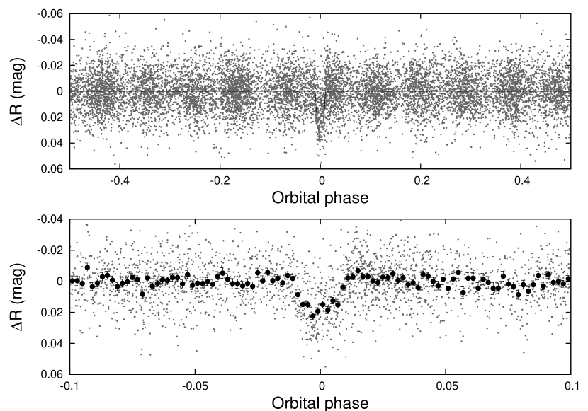
Figure 1.— Unbinned light curve of HAT-P-18 including all 10,000 instrumental $I$-band 5.5 minute cadence measurements obtained with the HAT-6 and HAT-9 telescopes of HATNet (see Table 1), and folded with the period $P=5.5080228$ days resulting from the global fit described in Section 3. The solid line shows a simplified transit model fit to the light curve (Section 3.3). The bold points in the lower panel show the light curve binned in phase with a bin-size of 0.002.

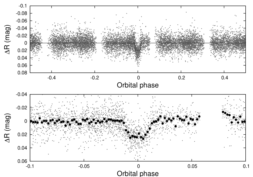
Figure 2.— Unbinned light curve of HAT-P-19 including all 10,000 instrumental $R$-band 5.5 minute cadence measurements obtained with the HAT-6, HAT-7, HAT-8 and HAT-9 telescopes of HATNet (see Table 1), and folded with the period $P=4.0087782$ days resulting from the global fit described in Section 3. The solid line shows a simplified transit model fit to the light curve (Section 3.3). The bold points in the lower panel show the light curve binned in phase with a bin-size of 0.002.

Table 1 Summary of photometric observations

Instrument/Field	Date(s)	Number of Images	Cadence (s)	Filter
HAT-P-18
HAT-6/G239	2007 Mar–2007 Jun	4383	330	$I$
HAT-9/G239	2007 Mar–2007 Jun	5719	330	$I$
KeplerCam	2008 Apr 25	215	73	Sloan $i$
KeplerCam	2009 May 10	185	133	Sloan $g$
HAT-P-19
HAT-7/G163	2007 Sep–2008 Jan	2324	330	$R$
HAT-8/G163	2007 Sep–2008 Jan	1617	330	$R$
HAT-6/G164	2007 Sep–2008 Feb	3676	330	$R$
HAT-9/G164	2007 Sep–2008 Feb	2711	330	$R$
KeplerCam	2009 Oct 06	37	84	Sloan $i$
KeplerCam	2009 Oct 30	97	150	Sloan $i$
KeplerCam	2009 Nov 27	76	84	Sloan $i$
KeplerCam	2009 Dec 01	194	89	Sloan $i$

2.2. Reconnaissance Spectroscopy

As is routine in the HATNet project, all candidates are subjected to careful scrutiny before investing valuable time on large telescopes. This includes spectroscopic observations at relatively modest facilities to establish whether the transit-like feature in the light curve of a candidate might be due to astrophysical phenomena other than a planet transiting a star. Many of such false positives are associated with large RV variations in the star (tens of $\rm km\,s^{-1}$) that are easily recognized. We made use of three different facilities to conduct these observations, including the Harvard-Smithsonian Center for Astrophysics (CfA) Digital Speedometer (DS; Latham, 1992), and the Tillinghast Reflector Echelle Spectrograph (TRES; Füresz, G., 2008), both on the 1.5 m Tillinghast Reflector at the Whipple Observatory on Mount Hopkins, Arizona, and the FIbre-fed Échelle Spectrograph (FIES; Frandsen & Lindberg, 1999) on the 2.5 m Nordic Optical Telescope (NOT; Djupvik & Andersen, 2010) at La Palma, Spain. We used these facilities to obtain high-resolution spectra, with typically low signal-to-noise (S/N) ratios that are nevertheless sufficient to derive RVs with moderate precisions of 0.5–1.0 $\rm km\,s^{-1}$ for slowly rotating stars. We also use these spectra to estimate the effective temperatures, surface gravities, and projected rotational velocities of the stars. With these observations we are able to reject many types of false positives, such as F dwarfs orbited by M dwarfs, grazing eclipsing binaries, or triple or quadruple star systems. Additional tests are performed with other spectroscopic material described in the next section. The observations and results for both stars are summarized in Table 2. Below we provide a brief description of each of the instruments used, the data reduction, and the analysis procedure.

We used the DS to conduct observations of both HAT-P-18 and HAT-P-19. This instrument delivers high-resolution spectra ($\lambda/\Delta\lambda\approx 35,\!000$) over a single order centered on the Mg I b triplet ($\sim$5187 Å). We measure the RV and stellar atmospheric parameters from the spectra following the method described by Torres et al. (2002).

We used FIES to conduct observations of HAT-P-19. We used the medium and the high-resolution fibers with resolving powers of $\lambda/\Delta\lambda\approx 46,\!000$ and $67,\!000$ respectively, giving a wavelength coverage of $\sim$ 3600-7400 Å. The spectra were extracted and analyzed to measure the RV and stellar atmospheric parameters following the procedures described by Buchhave et al. (2010). The velocities were corrected to the same system as the DS observations (heliocentric velocities with the gravitational redshift of the Sun subtracted) using 10 observations of the velocity standard HD 182488 obtained on the same nights as observations of HAT-P-19.

A single observation of HAT-P-19 was obtained with TRES. We used the medium-resolution fiber to obtain a spectrum with a resolution of $\lambda/\Delta\lambda\approx 44,000$ and a wavelength coverage of $\sim$ 3900-8900 Å. The spectrum was extracted and analyzed in a similar manner to the FIES observations. The velocity was corrected to the same system as the DS observations using a single TRES measurement of HD 182488 obtained on the same night. The velocity uncertainty reported in this case is our estimate of the systematic error based on the rms of multiple observations of HD 182488 obtained on other nights close in time.

Based on the reconnaissance spectroscopy observations we find that both systems have rms residuals consistent with no detectable RV variation within the precision of the measurements. All spectra were single-lined, i.e., there is no evidence that either target star has a stellar companion. Additionally, both stars have surface gravity measurements which indicate that they are dwarfs. We note that for HAT-P-19 all three instruments yielded similar results for the RV and stellar parameters. There is a $\sim 1$ $\rm km\,s^{-1}$ difference between the DS and the TRES/FIES observations of HAT-P-19. The last DS observation was obtained only four nights before the first FIES observation, and the DS and FIES data-sets each span significantly more than four nights, but do not show internal variations at the $\sim 1$ $\rm km\,s^{-1}$ level. We conclude that the velocity difference between the instruments does not indicate a physical variation in the velocity of HAT-P-19. The DS observations are all weak, with only a few counts per pixel, and the sky velocity is slightly more negative than the system velocity in all cases. This velocity difference may be due to a systematic error in the DS velocities due to sky contamination.

Table 2 Summary of reconnaissance spectroscopy observations

Instrument	Date(s)	Number of Spectra	$T_{\rm eff\star}$	$\log{g_{\star}}$	$v\sin{i}$	$\gamma_{\rm RV}$
			(K)	(cgs)	($\rm km\,s^{-1}$)	($\rm km\,s^{-1}$)
HAT-P-18
DS	2007 Sep–2008 Mar	4	$4750\pm 100$	$4.50\pm 0.25$	$1.5\pm 1.0$	$-11.92\pm 0.28$
HAT-P-19
DS	2008 Dec–2009 Jan	3	$4875\pm 125$	$4.25\pm 0.25$	$5\pm 5$	$-21.2\pm 0.5$
TRES	2009 Sep 04	1	$5000\pm 125$	$4.5\pm 0.25$	$2\pm 2$	$-20.20\pm 0.05$
FIES	2009 Jan–2009 Oct	7	$4875\pm 133$	$4.25\pm 0.27$	$2.1\pm 2$	$-20.22\pm 0.02$

2.3. High resolution, high S/N spectroscopy

We proceeded with the follow-up of each candidate by obtaining high-resolution, high-S/N spectra to characterize the RV variations, and to refine the determination of the stellar parameters. These observations are summarized in Table 3. The RV measurements and uncertainties for HAT-P-18 are given in Table 4, and for HAT-P-19 in Table 5. The period-folded data, along with our best fit described below in Section 3, are displayed in Figure 3 for HAT-P-18, and in Figure 4 for HAT-P-19. For HAT-P-18, we exclude five RV measurements that are significant outliers from the best fit model. These points are all strongly affected by contamination from scattered moonlight (see Section 3.2.1). Below we briefly describe the instruments used, the data reduction, and the analysis procedure.

Table 3 Summary of high-resolution/high-SN spectroscopic observations

Instrument	Date(s)	Number of
		RV obs.
HAT-P-18
Keck/HIRES	2007 Oct–2010 Mar	29
HAT-P-19
Keck/HIRES	2009 Oct–2010 Feb	13
Subaru/HDS	2009 Aug 8–2009 Aug 10	26

Observations were made of HAT-P-18 and HAT-P-19 with the HIRES instrument (Vogt et al., 1994) on the Keck I telescope located on Mauna Kea, Hawaii. The width of the spectrometer slit was $0\farcs 86$, resulting in a resolving power of $\lambda/\Delta\lambda\approx 55,\!000$, with a wavelength coverage of $\sim$3800–8000 Å. Exposures were obtained through an iodine gas absorption cell, which was used to superimpose a dense forest of $\mathrm{I}_{2}$ lines on the stellar spectrum and establish an accurate wavelength fiducial (see Marcy & Butler, 1992). For each target two additional exposures were taken without the iodine cell; in both cases we used the second, higher S/N, observation as the template in the reductions. Relative RVs in the solar system barycentric frame were derived as described by Butler et al. (1996), incorporating full modeling of the spatial and temporal variations of the instrumental profile.

We also made use of the High-Dispersion Spectrograph (HDS; Noguchi et al., 2002) on the Subaru telescope on Mauna Kea, Hawaii to obtain high-S/N spectroscopic observations of HAT-P-19 from which we derived high-precision RV measurements. Observations were made over three consecutive nights using a slit width of $0\farcs 6$, yielding a resolving power of $\lambda/\Delta\lambda\approx 60,\!000$. We used the I2b setup which provides a wavelength coverage of $\sim 3500-6200$ Å. To reduce the effect of changes in the barycentric velocity correction during an exposure, we limited exposure times to 15 minutes. As for Keck/HIRES, we made use of an iodine gas absorption cell to establish an accurate wavelength fiducial for each exposure. We also obtained six spectra without the iodine cell, which were combined to form the template observation. The spectra were extracted, and reduced to relative RVs in the solar system barycentric frame following the methods described by Sato et al. (2002, 2005).

Figure 3.— Top panel: Keck/HIRES RV measurements for HAT-P-18 shown as a function of orbital phase, along with our best-fit model (see Table 9). Zero phase corresponds to the time of mid-transit. The center-of-mass velocity has been subtracted. Second panel: Velocity $O\!-\!C$ residuals from the best fit. The error bars include a component from velocity jitter ($5.0$ $\rm m\,s^{-1}$) added in quadrature to the formal errors (see Section 3.3). Third panel: Bisector spans (BS), with the mean value subtracted. The measurement from the template spectrum is included (see Section 3.2.1). These measurements have not been corrected for contamination from moonlight; the corrected BS are shown in Figure 8. Bottom panel: Relative chromospheric activity index $S$ measured from the Keck spectra. The formal errors on $S$ based on photon statistics are comparable to the size of the displayed symbols. The scatter, however, is likely dominated by systematic errors in the measurements. Note the different vertical scales of the panels.

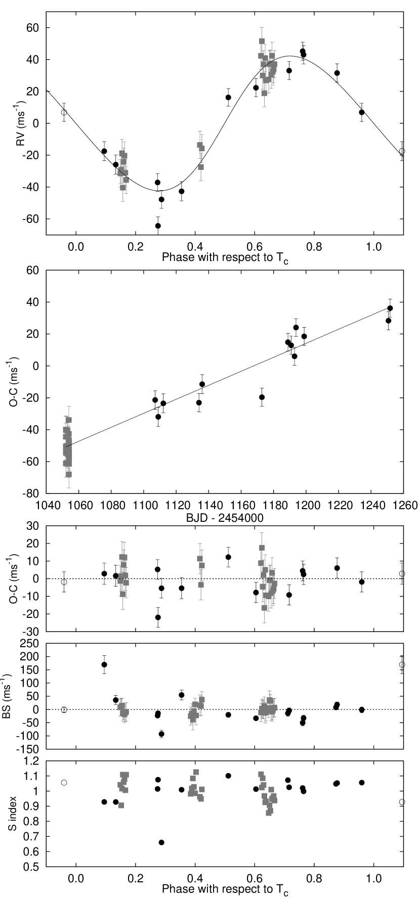
Figure 4.— Top panel: High-precision RV measurements for HAT-P-19 from Keck/HIRES (dark filled circles) and Subaru/HDS (light filled squares) shown as a function of orbital phase, along with our best-fit model (see Table 9). Zero phase corresponds to the time of mid-transit. The center-of-mass velocity and a linear trend (second panel) have been subtracted. Second panel: Velocity $O\!-\!C$ residuals from the best fit single Keplerian orbit model as a function of time. The residuals show a linear trend, indicative of a third body in the system. Note that the velocity zero points of the Subaru and Keck observations are independently free parameters. The linear trend is thus not constrained by the Subaru observations which span only 3 days. Third panel: Velocity $O\!-\!C$ residuals from the best fit including both the Keplerian orbit and linear trend, shown as a function of orbital phase. The error bars include a component from velocity jitter ($6.7$ $\rm m\,s^{-1}$) added in quadrature to the formal errors (see Section 3.3). Fourth panel: Bisector spans (BS), with the mean value subtracted. The measurement from the template spectrum is included (see Section 3.2.1). These measurements have not been corrected for contamination from moonlight; the corrected BS are shown in Figure 8. Bottom panel: Relative chromospheric activity index $S$ measured from the Keck spectra. The formal errors on $S$ based on photon statistics are comparable to the size of the displayed symbols. The scatter, however, is likely dominated by systematic errors in the measurements. Note the different vertical scales of the panels. Observations shown twice are represented with open symbols.

In each figure we show also the relative $S$ index, which is a measure of the chromospheric activity of the star derived from the flux in the cores of the Ca II H and K lines. This index was computed following the prescription given by Vaughan, Preston & Wilson (1978), after matching each spectrum to a reference spectrum using a transformation that includes a wavelength shift and a flux scaling that is a polynomial as a function of wavelength. The transformation was determined on regions of the spectra that are not used in computing this indicator. Note that our relative $S$ index has not been calibrated to the scale of Vaughan, Preston & Wilson (1978). We do not detect any significant variation of the index correlated with orbital phase; such a correlation might have indicated that the RV variations could be due to stellar activity, casting doubt on the planetary nature of the candidate.

Table 4 Relative radial velocities, bisector spans, and activity index measurements of HAT-P-18.

BJD	RV	$\sigma_{\rm RV}$	BS	$\sigma_{\rm BS}$	S	$\sigma_{\rm S}$
(2,454,000$+$)	($\rm m\,s^{-1}$)	($\rm m\,s^{-1}$)	($\rm m\,s^{-1}$)	($\rm m\,s^{-1}$)
$397.73420$	$-11.23$	$3.79$	$-28.29$	$13.90$	$0.8595$	$0.0099$
$548.08129$	$\cdots$	$\cdots$	$14.12$	$20.54$	$0.9267$	$0.0051$
$548.09633$	$25.83$	$2.26$	$-2.20$	$26.16$	$0.9344$	$0.0057$
$549.07743$	$22.80$	$2.27$	$3.36$	$14.43$	$0.9748$	$0.0048$
$602.83762$	$9.95$	$2.25$	$67.02$	$28.63$	$1.0102$	$0.0048$
$602.99835$	$15.96$	$2.29$	$12.79$	$12.66$	$1.0183$	$0.0045$
$603.83449$	$20.24$	$2.72$	$141.82$	$43.52$	$1.0057$	$0.0061$
$604.08627$	$10.30$	$2.51$	$-27.50$	$9.88$	$1.0266$	$0.0049$
$633.97708$	$-21.65$	$2.45$	$9.96$	$12.03$	$1.0472$	$0.0146$
$635.98889$	$20.26$	$2.69$	$52.95$	$10.05$	$0.9688$	$0.0058$
$639.02280$	$-25.53$	$2.29$	$-8.96$	$6.28$	$0.9811$	$0.0058$
$641.97905$	$31.77$	$2.88$	$-20.46$	$13.72$	$1.0007$	$0.0075$
$724.84068\tablenotemark{e}$	$6.49$	$3.39$	$-198.81$	$36.35$	$0.9206$	$0.0158$
$726.79620$	$-27.63$	$2.46$	$-72.66$	$14.74$	$0.9544$	$0.0091$
$727.79088$	$-26.34$	$2.31$	$-47.93$	$16.52$	$0.9805$	$0.0078$
$777.69605$	$-16.44$	$2.46$	$26.52$	$7.61$	$0.9408$	$0.0076$
$778.69476\tablenotemark{e}$	$35.06$	$3.21$	$45.44$	$11.89$	$0.8932$	$0.0127$
$779.70147\tablenotemark{e}$	$56.60$	$4.98$	$60.37$	$20.83$	$0.8978$	$0.0212$
$779.74051\tablenotemark{e}$	$61.15$	$5.71$	$134.75$	$51.14$	$0.8017$	$0.0458$
$865.15876$	$-25.60$	$4.88$	$-31.22$	$22.33$	$1.0424$	$0.0166$
$955.02444$	$14.38$	$2.41$	$-19.22$	$14.02$	$1.0448$	$0.0056$
$955.96262$	$30.73$	$2.64$	$-17.35$	$10.67$	$1.0609$	$0.0050$
$964.09646$	$-33.57$	$2.32$	$18.65$	$11.88$	$0.9697$	$0.0047$
$987.98665$	$20.65$	$2.88$	$76.71$	$20.29$	$1.0195$	$0.0057$
$988.90490$	$29.18$	$2.82$	$91.83$	$24.70$	$1.0630$	$0.0058$
$1109.76458\tablenotemark{e}$	$-49.58$	$3.25$	$-135.43$	$28.38$	$0.7973$	$0.0308$
$1016.99998$	$30.57$	$2.20$	$-25.04$	$8.82$	$1.0197$	$0.0076$
$1041.96078$	$-13.06$	$3.12$	$-12.39$	$11.79$	$1.0428$	$0.0162$
$1252.06235$	$-3.90$	$2.92$	$-45.97$	$12.38$	$1.0616$	$0.0065$
$1252.07745$	$\cdots$	$\cdots$	$-34.63$	$6.47$	$1.0437$	$0.0055$
$1261.11905$	$-19.39$	$2.39$	$-28.25$	$12.16$	$1.0019$	$0.0053$

Note. — Note that for the iodine-free template exposures we do not measure the RV but do measure the BS and S index. Such template exposures can be distinguished by the missing RV value.

Table 5 Relative radial velocities, bisector spans, and activity index measurements of HAT-P-19.

BJD	RV	$\sigma_{\rm RV}$	BS	$\sigma_{\rm BS}$	S	$\sigma_{\rm S}$	Inst.
(2,454,000$+$)	($\rm m\,s^{-1}$)	($\rm m\,s^{-1}$)	($\rm m\,s^{-1}$)	($\rm m\,s^{-1}$)
$1052.04317$	$-83.78$	$7.01$	$7.91$	$33.17$	$1.042$	$0.324$	Subaru
$1052.05438$	$-81.45$	$6.85$	$9.71$	$30.12$	$0.905$	$0.294$	Subaru
$1052.06559$	$-71.03$	$6.92$	$14.66$	$27.93$	$1.016$	$0.315$	Subaru
$1052.07680$	$-92.65$	$6.96$	$-14.95$	$29.17$	$1.109$	$0.328$	Subaru
$1052.08801$	$-76.43$	$6.91$	$-8.57$	$29.23$	$1.059$	$0.330$	Subaru
$1052.09923$	$-72.59$	$6.90$	$-18.67$	$31.68$	$1.079$	$0.329$	Subaru
$1052.11044$	$-83.27$	$6.87$	$-11.72$	$33.40$	$1.006$	$0.304$	Subaru
$1052.12165$	$-87.81$	$6.88$	$-8.79$	$35.31$	$1.108$	$0.340$	Subaru
$1052.99045$	$\cdots$	$\cdots$	$-25.11$	$34.01$	$0.982$	$0.313$	Subaru
$1053.00513$	$\cdots$	$\cdots$	$-15.75$	$37.37$	$1.018$	$0.318$	Subaru
$1053.01981$	$\cdots$	$\cdots$	$-38.58$	$39.13$	$1.083$	$0.330$	Subaru
$1053.03449$	$\cdots$	$\cdots$	$-6.01$	$32.64$	$1.028$	$0.332$	Subaru
$1053.04918$	$\cdots$	$\cdots$	$19.45$	$23.05$	$0.986$	$0.315$	Subaru
$1053.06386$	$\cdots$	$\cdots$	$-22.72$	$35.09$	$1.126$	$0.347$	Subaru
$1053.11425$	$-65.38$	$6.90$	$15.97$	$38.62$	$0.962$	$0.309$	Subaru
$1053.12894$	$-79.28$	$6.85$	$13.01$	$37.16$	$0.948$	$0.313$	Subaru
$1053.14023$	$-67.57$	$7.11$	$37.01$	$30.50$	$1.011$	$0.331$	Subaru
$1053.93729$	$-9.14$	$6.91$	$-11.41$	$35.52$	$1.111$	$0.338$	Subaru
$1053.94850$	$0.07$	$6.93$	$2.85$	$33.24$	$1.023$	$0.320$	Subaru
$1053.95970$	$-21.48$	$6.88$	$3.11$	$36.49$	$1.085$	$0.334$	Subaru
$1053.97091$	$-14.40$	$6.87$	$-1.28$	$34.68$	$1.040$	$0.314$	Subaru
$1053.98213$	$-32.56$	$6.87$	$12.91$	$33.85$	$0.968$	$0.301$	Subaru
$1053.99335$	$-10.54$	$6.84$	$-12.62$	$38.43$	$0.926$	$0.304$	Subaru
$1054.00457$	$-24.54$	$6.83$	$-10.77$	$32.87$	$0.933$	$0.306$	Subaru
$1054.04057$	$-23.88$	$6.80$	$5.45$	$35.97$	$0.855$	$0.273$	Subaru
$1054.05178$	$-14.33$	$6.78$	$35.76$	$34.71$	$0.907$	$0.295$	Subaru
$1054.06300$	$-13.93$	$6.82$	$32.75$	$23.55$	$0.870$	$0.285$	Subaru
$1054.07421$	$-20.91$	$6.81$	$-4.30$	$35.97$	$1.009$	$0.323$	Subaru
$1054.08543$	$-9.03$	$6.81$	$-8.63$	$35.77$	$0.947$	$0.310$	Subaru
$1054.09665$	$-18.96$	$6.75$	$-3.25$	$35.11$	$0.953$	$0.304$	Subaru
$1054.10787$	$-17.49$	$6.78$	$5.49$	$35.24$	$0.967$	$0.308$	Subaru
$1054.11908$	$-14.29$	$6.82$	$7.07$	$34.89$	$0.937$	$0.297$	Subaru
$1107.06075$	$\cdots$	$\cdots$	$7.74$	$7.81$	$1.048$	$0.011$	Keck
$1107.07559$	$4.11$	$2.77$	$18.29$	$9.69$	$1.053$	$0.044$	Keck
$1108.99050$	$-69.19$	$3.09$	$54.83$	$18.48$	$1.009$	$0.014$	Keck
$1112.11372$	$-51.05$	$3.13$	$35.61$	$17.65$	$0.928$	$0.020$	Keck
$1134.04526$	$7.06$	$2.60$	$-33.21$	$6.43$	$1.013$	$0.024$	Keck
$1136.01174$	$-31.79$	$3.10$	$169.45$	$34.81$	$0.928$	$0.034$	Keck
$1172.81382$	$-61.98$	$2.36$	$-14.18$	$3.85$	$1.075$	$0.011$	Keck
$1188.84358$	$-27.51$	$2.19$	$-22.96$	$5.20$	$1.014$	$0.010$	Keck
$1190.80886$	$53.47$	$2.62$	$-32.46$	$11.07$	$0.998$	$0.011$	Keck
$1192.90496$	$-36.33$	$2.34$	$-92.65$	$14.20$	$0.660$	$0.020$	Keck
$1193.80419$	$28.07$	$2.18$	$-20.27$	$8.65$	$1.101$	$0.011$	Keck
$1198.81373$	$59.29$	$2.49$	$-50.27$	$11.66$	$1.020$	$0.010$	Keck
$1250.72949$	$\cdots$	$\cdots$	$-14.06$	$11.36$	$1.072$	$0.011$	Keck
$1250.74616$	$70.58$	$2.56$	$-4.56$	$10.41$	$1.025$	$0.015$	Keck
$1251.72400$	$44.90$	$2.60$	$-1.30$	$10.91$	$1.056$	$0.016$	Keck

Note. — Note that for the iodine-free template exposures we do not measure the RV but do measure the BS and S index. Such template exposures can be distinguished by the missing RV value.

2.4. Photometric follow-up observations

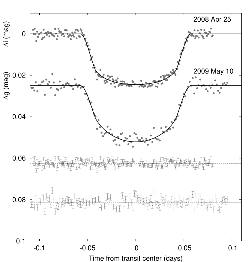
Figure 5.— Unbinned transit light curves for HAT-P-18, acquired with KeplerCam at the FLWO 1.2 m telescope. The light curves have been EPD and TFA processed, as described in § 3.3. The dates of the events are indicated. The second curve is displaced vertically for clarity. Our best fit from the global modeling described in Section 3.3 is shown by the solid lines. Residuals from the fits are displayed at the bottom, in the same order as the top curves. The error bars represent the photon and background shot noise, plus the readout noise.

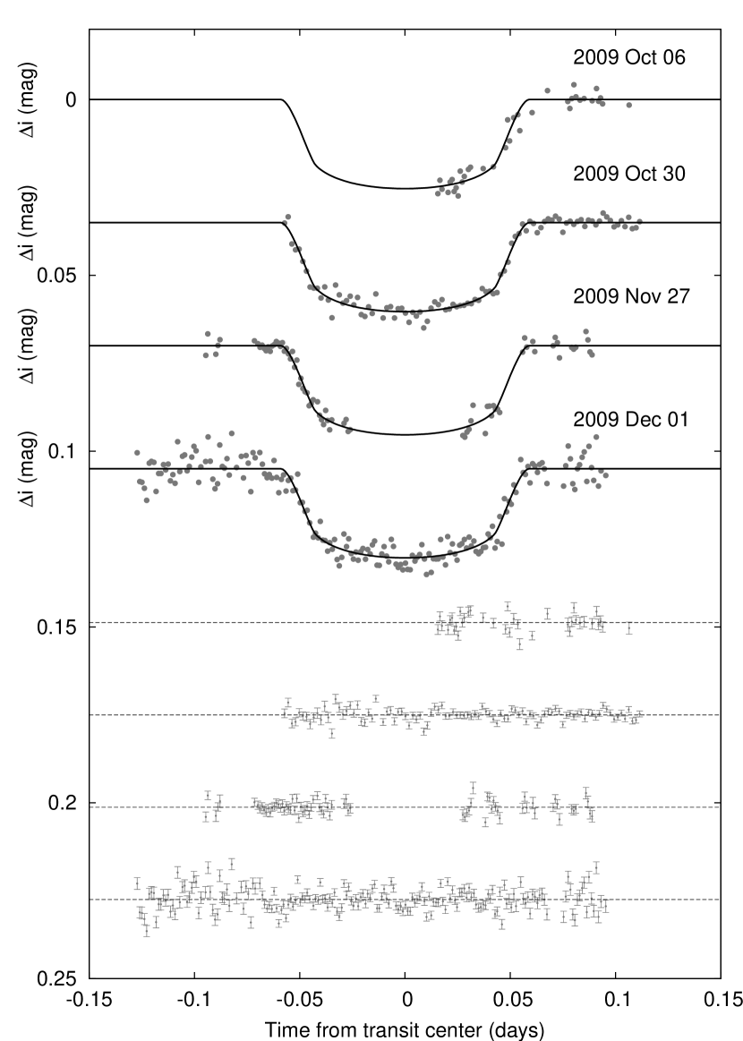
Figure 6.— Similar to Figure 5; here we show the follow-up light curves for HAT-P-19.

In order to permit a more accurate modeling of the light curves, we conducted additional photometric observations with the KeplerCam CCD camera on the FLWO 1.2 m telescope. The observations for each target are summarized in Table 1.

The reduction of these images, including basic calibration, astrometry, and aperture photometry, was performed as described by Bakos et al. (2010). We performed EPD and TFA to remove trends simultaneously with the light curve modeling (for more details, see Section 3, and Bakos et al., 2010). The final time series, together with our best-fit transit light curve model, are shown in the top portion of Figures 5 and 6 for HAT-P-18 and HAT-P-19 respectively; the individual measurements are reported in Tables 6 and 7.

Table 6 High-precision differential photometry of HAT-P-18.

BJD	Mag	$\sigma_{\rm Mag}$	Mag(orig)	Filter
(2,400,000$+$)
$54582.72249$	$-0.00198$	$0.00093$	$10.79530$	$i$
$54582.72334$	$0.00006$	$0.00093$	$10.79800$	$i$
$54582.72420$	$-0.00247$	$0.00093$	$10.79660$	$i$
$54582.72506$	$0.00024$	$0.00093$	$10.79950$	$i$
$54582.72592$	$0.00344$	$0.00093$	$10.80160$	$i$
$54582.72677$	$-0.00104$	$0.00093$	$10.79740$	$i$
$54582.72760$	$0.00148$	$0.00092$	$10.79980$	$i$
$54582.72848$	$0.00027$	$0.00092$	$10.79820$	$i$
$54582.72933$	$0.00002$	$0.00092$	$10.79590$	$i$
$54582.73102$	$-0.00066$	$0.00092$	$10.79560$	$i$

Note. — This table is available in a machine-readable form in the online journal. A portion is shown here for guidance regarding its form and content.

Table 7 High-precision differential photometry of HAT-P-19.

BJD	Mag	$\sigma_{\rm Mag}$	Mag(orig)	Filter
(2,400,000$+$)
$55111.59368$	$0.02677$	$0.00139$	$11.66270$	$i$
$55111.59465$	$0.02295$	$0.00130$	$11.65390$	$i$
$55111.59562$	$0.02551$	$0.00142$	$11.65450$	$i$
$55111.59853$	$0.02643$	$0.00133$	$11.66000$	$i$
$55111.59949$	$0.02348$	$0.00120$	$11.65220$	$i$
$55111.60045$	$0.02275$	$0.00140$	$11.65930$	$i$
$55111.60140$	$0.02615$	$0.00126$	$11.65320$	$i$
$55111.60236$	$0.02510$	$0.00126$	$11.65380$	$i$
$55111.60333$	$0.02741$	$0.00130$	$11.66230$	$i$
$55111.60430$	$0.02038$	$0.00121$	$11.64810$	$i$

Note. — This table is available in a machine-readable form in the online journal. A portion is shown here for guidance regarding its form and content.

3. Analysis

3.1. Properties of the parent star

Fundamental parameters for each of the host stars, including the mass ($M_{\star}$) and radius ($R_{\star}$), which are needed to infer the planetary properties, depend strongly on other stellar quantities that can be derived spectroscopically. For this we have relied on our template spectra obtained with the Keck/HIRES instrument, and the analysis package known as Spectroscopy Made Easy (SME; Valenti & Piskunov, 1996), along with the atomic line database of Valenti & Fischer (2005). For each star, SME yielded the following initial values and uncertainties (which we have conservatively increased by a factor of two to include our estimates of the systematic errors):

• HAT-P-18 – effective temperature $T_{\rm eff\star}=$$4850\pm 75$ K, stellar surface gravity $\log{g_{\star}}=$$4.7\pm 0.1$ (cgs), metallicity $\rm[Fe/H]=$$+0.12\pm 0.05$ dex, and projected rotational velocity $v\sin{i}=$$1.2\pm 0.5$ $\rm km\,s^{-1}$.

• HAT-P-19 – effective temperature $T_{\rm eff\star}=$$5037\pm 44$ K, stellar surface gravity $\log{g_{\star}}=$$4.7\pm 0.1$ (cgs), metallicity $\rm[Fe/H]=$$+0.24\pm 0.03$ dex, and projected rotational velocity $v\sin{i}=$$2.4\pm 0.5$ $\rm km\,s^{-1}$.

As discussed in Section 3.2.1, contamination from scattered moonlight affects the bisector spans and radial velocities measured for HAT-P-18 and the bisector spans measured for HAT-P-19. For HAT-P-18 the moon was below the horizon when the template used for the SME analysis was obtained, so it is not affected by contamination. For HAT-P-19 we estimate that scattered moonlight may have contributed $\sim 0.1\%$ of the total flux to the template spectrum used for SME analysis. The error in the parameters that results from this contamination is likely dwarfed by other systematic errors in the parameter determination.

In principle the effective temperature and metallicity, along with the surface gravity taken as a luminosity indicator, could be used as constraints to infer the stellar mass and radius by comparison with stellar evolution models. However, the effect of $\log{g_{\star}}$ on the spectral line shapes is rather subtle, and as a result it is typically difficult to determine accurately, so that it is a rather poor luminosity indicator in practice. For planetary transits a stronger constraint is often provided by the $a/R_{\star}$ normalized semimajor axis, which is closely related to $\rho_{\star}$, the mean stellar density. The quantity $a/R_{\star}$ can be derived directly from the transit light curves (see Sozzetti et al., 2007, and also Section 3.3). This, in turn, allows us to improve on the determination of the spectroscopic parameters by supplying an indirect constraint on the weakly determined spectroscopic value of $\log{g_{\star}}$, which removes degeneracies. We take this approach here, as described below. The validity of our assumption, namely that the best physical model describing our data is a planetary transit (as opposed to a blend), is shown later in Section 3.2.1.

For each system, our initial values of $T_{\rm eff\star}$, $\log{g_{\star}}$, and $\rm[Fe/H]$ were used to determine auxiliary quantities needed in the global modeling of the follow-up photometry and radial velocities (specifically, the limb-darkening coefficients). This modeling, the details of which are described in Section 3.3, uses a Monte Carlo approach to deliver the numerical probability distribution of $a/R_{\star}$ and other fitted variables. For further details we refer the reader to Pál (2009b). When combining $a/R_{\star}$ (used as a proxy for luminosity) with assumed Gaussian distributions for $T_{\rm eff\star}$ and $\rm[Fe/H]$ based on the SME determinations, a comparison with stellar evolution models allows the probability distributions of other stellar properties to be inferred, including $\log{g_{\star}}$. Here we use the stellar evolution calculations from Yonsei-Yale (YY; Yi et al., 2001) for both stars. The comparison against the model isochrones was carried out for each of 10,000 Monte Carlo trial sets for HAT-P-18, and 20,000 Monte Carlo trial sets for HAT-P-19 (see Section 3.3). Parameter combinations corresponding to unphysical locations in the H-R diagram (41% of the trials for HAT-P-18 and 31% of the trials for HAT-P-19) were ignored, and replaced with another randomly drawn parameter set. For each system we carried out a second SME iteration in which we adopted the value of $\log{g_{\star}}$ so determined and held it fixed in a new SME analysis (coupled with a new global modeling of the RV and light curves), adjusting only $T_{\rm eff\star}$, $\rm[Fe/H]$, and $v\sin{i}$. This gave

• HAT-P-18 – $T_{\rm eff\star}=$$4803\pm 80$ K, $\log{g_{\star}}=$$4.56\pm 0.06$, $\rm[Fe/H]=$$+0.10\pm 0.08$, and $v\sin{i}=$$0.5\pm 0.5$ $\rm km\,s^{-1}$.

• HAT-P-19 – $T_{\rm eff\star}=$$4990\pm 130$ K, $\log{g_{\star}}=$$4.53\pm 0.06$ (fixed), $\rm[Fe/H]=$$+0.23\pm 0.08$, and $v\sin{i}=$$0.7\pm 0.5$ $\rm km\,s^{-1}$.

In each case the conservative uncertainties for $T_{\rm eff\star}$ and $\rm[Fe/H]$ have been increased by a factor of two over their formal values, as before. For each system, a further iteration did not change $\log{g_{\star}}$ significantly, so we adopted the values stated above, together with the new $\log{g_{\star}}$ values resulting from the global modeling, as the final atmospheric properties of the stars. They are collected in Table 8 for both stars.

With the adopted spectroscopic parameters the model isochrones yield the stellar mass and radius, and other properties. These are listed for each of the systems in Table 8. According to these models HAT-P-18 is a dwarf star with an estimated age of $12.4_{-6.4}^{+4.4}$ Gyr, and HAT-P-19 is a dwarf star with an estimated age of $8.8\pm 5.2$ Gyr. The inferred location of each star in a diagram of $a/R_{\star}$ versus $T_{\rm eff\star}$, analogous to the classical H-R diagram, is shown in Figure 7. The stellar properties and their 1$\sigma$ and 2$\sigma$ confidence ellipsoids are displayed against the backdrop of model isochrones for a range of ages, and the appropriate stellar metallicity. For comparison, the locations implied by the initial SME results are also shown with triangles.

Figure 7.— Left: model isochrones from Yi et al. (2001) for the measured metallicity of HAT-P-18, $\rm[Fe/H]$= $+0.10$, and ages of 0.2, 0.5, and 1 to 14 Gyr, in 1 Gyr increments (left to right). The adopted values of $T_{\rm eff\star}$ and $a/R_{\star}$ are shown together with their 1$\sigma$ and 2$\sigma$ confidence ellipsoids. The initial values of $T_{\rm eff\star}$ and $a/R_{\star}$ from the first SME and light curve analyses are represented with a triangle. Right: same as left, here we show the results for HAT-P-19, with $\rm[Fe/H]$= $+0.23$, and ages of 1 to 13 Gyr in steps of 1 Gyr (left to right).

The stellar evolution modeling provides color indices that may be compared against the measured values as a sanity check. For each star, the best available measurements are the near-infrared magnitudes from the 2MASS Catalogue (Skrutskie et al., 2006), which are given in Table 8. These are converted to the photometric system of the models (ESO system) using the transformations by Carpenter (2001). The resulting color index is $J-K=0.623\pm 0.036$, and $J-K=0.583\pm 0.031$ for HAT-P-18, and HAT-P-19 respectively. These are both within $1\sigma$ of the predicted values from the isochrones of $J-K=0.61\pm 0.02$ and $J-K=0.57\pm 0.03$. The distance to each object may be computed from the absolute $K$ magnitude from the models and the 2MASS $K_{s}$ magnitudes, which has the advantage of being less affected by extinction than optical magnitudes. The results are given in Table 8, where in each case the uncertainty excludes possible systematics in the model isochrones that are difficult to quantify.

Table 8 Stellar parameters for HAT-P-18 and HAT-P-19

Parameter	HAT-P-18	HAT-P-19	Source
Spectroscopic properties
$T_{\rm eff\star}$ (K)	$4803\pm 80$	$4990\pm 130$	SME
$\rm[Fe/H]$	$+0.10\pm 0.08$	$+0.23\pm 0.08$	SME
$v\sin{i}$ ($\rm km\,s^{-1}$)	$0.5\pm 0.5$	$0.7\pm 0.5$	SME
$v_{\rm mac}$ ($\rm km\,s^{-1}$)	$2.53$	$2.81$	SME
$v_{\rm mic}$ ($\rm km\,s^{-1}$)	$0.85$	$0.85$	SME
$\gamma_{\rm RV}$ ($\rm km\,s^{-1}$)	$-11.92\pm 0.28$	$-20.22\pm 0.02$	DS/FIES
Photometric properties
$V$ (mag)	12.759	12.901	TASS
$V\!-\!I_{C}$ (mag)	$1.18\pm 0.13$	$1.04\pm 0.13$	TASS
$J$ (mag)	$10.822\pm 0.020$	$11.095\pm 0.020$	2MASS
$H$ (mag)	$10.340\pm 0.019$	$10.644\pm 0.022$	2MASS
$K_{s}$ (mag)	$10.234\pm 0.017$	$10.546\pm 0.019$	2MASS
Derived properties
$M_{\star}$ ($M_{\sun}$)	$0.770\pm 0.031$	$0.842\pm 0.042$	YY+$a/R_{\star}$+SME
$R_{\star}$ ($R_{\sun}$)	$0.749\pm 0.037$	$0.820\pm 0.048$	YY+$a/R_{\star}$+SME
$\log{g_{\star}}$ (cgs)	$4.57\pm 0.04$	$4.54\pm 0.05$	YY+$a/R_{\star}$+SME
$L_{\star}$ ($L_{\sun}$)	$0.27\pm 0.04$	$0.37_{-0.06}^{+0.08}$	YY+$a/R_{\star}$+SME
$M_{V}$ (mag)	$6.50\pm 0.19$	$6.08\pm 0.24$	YY+$a/R_{\star}$+SME
$M_{K}$ (mag,ESO)	$4.17\pm 0.12$	$3.92\pm 0.15$	YY+$a/R_{\star}$+SME
Age (Gyr)	$12.4_{-6.4}^{+4.4}$	$8.8\pm 5.2$	YY+$a/R_{\star}$+SME
Distance (pc)	$166\pm 9$	$215\pm 15$	YY+$a/R_{\star}$+SME

3.2. Rejecting Blend Scenarios

Our initial spectroscopic analyses discussed in Section 2.2 and Section 2.3 rule out the most obvious astrophysical false positive scenarios. However, more subtle phenomena such as blends (contamination by an unresolved eclipsing binary, whether in the background or associated with the target) can still mimic both the photometric and spectroscopic signatures we see. In the following sections we consider and rule out the possibility that such scenarios may have caused the observed photometric and spectroscopic features.

3.2.1 Spectral line-bisector analysis

Following Torres et al. (2007), we explored the possibility that the measured radial velocities are not real, but are instead caused by distortions in the spectral line profiles due to contamination from a nearby unresolved eclipsing binary. A bisector analysis for each system based on the Keck spectra (and the Subaru spectra for HAT-P-19) was done as described in §5 of Bakos et al. (2007).

Each system shows excess scatter in the bisector spans (BS), above what is expected from the measurement errors (see Figure 3, third panel, and Figure 4, fourth panel). For HAT-P-18 there may be a slight correlation between the RV and the BS, while for HAT-P-19 no correlation is apparent. Such a correlation could indicate that the photometric and spectroscopic signatures are due to a blend scenario rather than a single planet transiting a single star. We note that for HAT-P-19, the Keck spectra show excess BS variation, while the Subaru spectra do not.

Following our earlier work (Kovács et al., 2010; Hartman et al., 2009) we investigated the effect of contamination from moonlight on the measured BS values. As in Kovács et al. (2010), we estimate the expected BS value for each spectrum by modeling the spectrum cross-correlation function (CCF) as the sum of two Lorentzian functions, shifted by the known velocity difference between the star and the moon, and scaled by their expected flux ratio (estimated following equation 3 of Hartman et al., 2009). We refer to the simulated BS value as the sky contamination factor (SCF). We find a strong correlation between the SCF and BS for both systems (see Figure 8). After correcting for this correlation, we find that the BS show no significant variations, and the correlation between the RV and BS variations is insignificant for both systems. Therefore, we conclude that the the velocity variations are real for both stars, and that both stars are orbited by close-in giant planets. An independent method for arriving at this same conclusion is also presented in the following section.

We have also investigated the effect of sky contamination on the measured RVs. The expected RV due to sky contamination for a given spectrum is estimated by finding the peak of the simulated CCF. Note that the real RV measurements are obtained by directly modeling the spectra and not by performing cross-correlation. We therefore only expect a crude agreement between the estimated RVs due to sky contamination, and the real RVs. Figure 9 compares the expected RVs to the measured RV residuals from the best-fit model for HAT-P-18 and HAT-P-19. For HAT-P-18 we find a rough correlation between the estimated and measured RV residuals. Five of the RV measurements which are significant outliers from the best-fit model are rejected. These spectra are also among the most strongly affected by sky contamination. For HAT-P-19 the values do not appear to be correlated.

Figure 8.— A: BS vs SCF for Keck spectra of HAT-P-18. The strong correlation between these quantities indicates that much of the BS variation for this object can be accounted for by changes in the sky contamination of the spectra. B: BS vs orbital phase for HAT-P-18 after fitting and subtracting a linear relation between BS and SCF. The residual BS is uncorrelated with the orbital phase, justifying our conclusion that this system is not a blend. Bottom: BS vs SCF for Keck spectra of HAT-P-19. Again the BS variation for this target can be accounted for by the changing sky contamination. The Subaru spectra of HAT-P-19 do not show significant BS variations; these spectra were taken within a span of 3 days, under similar sky conditions. D: Same as panel B, here shown for HAT-P-19.

Figure 9.— Top: Residual RV from best-fit model vs estimated RV due to sky contamination for Keck spectra of HAT-P-18. There is a rough correlation between the values. Open circles show RV outliers which were excluded when modeling the orbit, filled circles show all other measurements. The excluded measurements come from observations which are expected to be strongly contaminated by the sky. Bottom: Same as above, here we show the results for HAT-P-19. In this case there is no apparent correlation between the observed RV residuals and the expected RVs due to sky contamination.

3.2.2 Blend Modeling of the Photometry

As an independent test on the possibility that the observations for either HAT-P-18 or HAT-P-19 could be caused by a blend scenario, we follow Torres et al. (2005), Hartman et al. (2009), and Bakos et al. (2010) in attempting to model the photometric observations for each object as either a hierarchical triple system, or a blend between a bright foreground star and a background eclipsing binary. We will show that for both HAT-P-18 and HAT-P-19 blend scenarios that do not include a transiting planet may be rejected from the photometric observations alone. We consider 5 possibilities:

1. One star orbited by a planet,

2. Hierarchical system, 3 stars, 2 fainter stars are eclipsing,

3. Hierarchical system, 2 stars, 1 planet, planet orbits the fainter star,

4. Hierarchical system, 2 stars, 1 planet, planet orbits the brighter star,

5. Chance alignment, 3 stars, 2 background stars are eclipsing.

Here case 1 is the fiducial model to which we compare the various blend models. We model the observed follow-up and HATNet light curves (including only points that are within one transit duration of the primary transit or secondary eclipse assuming zero eccentricity) together with the 2MASS and TASS photometry. In all cases we vary the distance to the brightest star in the system, parameters allowing for dilution in the HATNet light curves, and we include simultaneous EPD and TFA in fitting the light curves (see Section 3.3). We draw the stellar radii and magnitudes from the Padova isochrones (Girardi et al., 2000), extended below 0.15 $M_{\sun}$ with the Baraffe et al. (1998) isochrones. We use these rather than the YY isochrones for this analysis because of the need to allow for stars with $M<0.4$ $M_{\sun}$, which is the lower limit available for the YY models. We use the JKTEBOP program (Southworth et al., 2004a, b) which is based on the Eclipsing Binary Orbit Program (EBOP; Popper & Etzel, 1981; Etzel, 1981; Nelson & Davis, 1972) to generate the model light curves. We optimize the free parameters using the Downhill Simplex Algorithm together with the classical linear least squares algorithm for the EPD and TFA parameters. We rescale the errors for each light curve such that $\chi^{2}$ per degree of freedom is 1.0 for the out of transit portion of the light curve. Note that this is done prior to applying EPD/TFA corrections for systematic errors. As a result, the $\chi^{2}$ per degree of freedom is less than 1.0 for many of the best-fit models discussed below. If the rescaling is not performed, the difference in $\chi^{2}$ between the best-fit models is even more significant than what is given below, and the blend models may be rejected with even higher confidence. For HAT-P-18 we fix the mass, age, and [Fe/H] metallicity of the brightest star in the system to $0.76$ $M_{\sun}$, $12.4$ Gyr, and $+0.10$ respectively to reproduce the effective temperature, metallicity, and surface gravity of the bright star as determined from the SME analysis when using the Padova isochrones. For HAT-P-19 we fix the mass, age, and metallicity to $0.83$ $M_{\sun}$, $8.8$ Gyr, and $+0.23$ respectively.

Case 1: 1 star, 1 planet: In addition to the parameters mentioned above, in this case we vary the radius of the planet and the impact parameter of the transit. For HAT-P-18 the best-fit model has $\chi^{2}_{\rm 18,Case1}=1542.4$ for 1712 degrees of freedom. For HAT-P-19 the best-fit model has $\chi^{2}_{\rm 19,Case1}=2710.0$ for 2746 degrees of freedom. The parameters that we obtain for both objects are comparable to those obtained from the global modelling described in Section 3.3.

Case 2: Hierarchical system, 3 stars: For case 2 we vary the masses of the eclipsing components, and the impact parameter of the eclipse. We take the radii and magnitudes of all three stars from the same isochrone. For HAT-P-18 we find $\chi^{2}_{\rm 18,Case2}=1566.9$ for 1711 degrees of freedom, while for HAT-P-19 we find $\chi^{2}_{\rm 19,Case2}=2753.6$ for 2745 degrees of freedom. The best-fit model for HAT-P-18 consists of a $0.76$ $M_{\sun}$ star that is blended with a eclipsing binary with components of mass $0.74$ $M_{\sun}$ and $0.12$ $M_{\sun}$. For HAT-P-19 the best-fit model consists of two equal $0.83$ $M_{\sun}$ stars with a $0.13$ $M_{\sun}$ M dwarf eclipsing one of the two K stars. For both HAT-P-18 and HAT-P-19 the best-fit case 2 model has higher $\chi^{2}$ with fewer degrees of freedom than the best-fit case 1 model, so for both objects the case 1 model is prefered. To establish the significance at which we may reject the Case 2 model in favor of the Case 1 model, we conduct Monte Carlo simulations which account for the possibility of uncorrected systematic errors in the light curves as described in Hartman et al. (2009). For HAT-P-18 we reject the best-fit Case 2 model at the $\sim 4.4\sigma$ confidence level, while for HAT-P-19 we reject the best-fit Case 2 model at the $\sim 5.1\sigma$ confidence level. We also note that for both objects the only hierarchical triple stellar system that could potentially fit the photometric observations is a system where the two brightest stars have nearly equal masses. Because both HAT-P-18 and HAT-P-19 have narrow spectral lines ($v\sin{i}=$$0.5\pm 0.5$ $\rm km\,s^{-1}$ and $0.7\pm 0.5$ $\rm km\,s^{-1}$ respectively), a second component with a luminosity ratio close to one and a RV semi-amplitude of several tens of $\rm km\,s^{-1}$ would have easily been detected in the spectra of these objects.

Case 3: Hierarchical system, 2 stars, 1 planet, planet orbits fainter star: In this scenario the system contains a transiting planet, but it would have a radius that is larger than what we infer assuming there is only one star in the system. For this case we vary the mass of the faint planet-hosting star, the radius of the planet, and the impact parameter of the transit. We assume the mass of the planet is negligible relative to the mass of its faint host star. For HAT-P-18 the best-fit Case 3 model has $\chi^{2}_{\rm 18,Case3}=1590.0$ while for HAT-P-19 the best-fit Case 3 model has $\chi^{2}_{\rm 19,Case3}=2726.1$. For both objects the best-fit is when the two stars in the system are of equal mass. Repeating the Monte Carlo simulations to determine the statistical significance of this $\chi^{2}$ difference, we find that for HAT-P-18 we may reject the Case 3 model in favor of the Case 1 model at the $\sim 4.9\sigma$ confidence level, while for HAT-P-19 we may reject the Case 3 model at the $\sim 3.6\sigma$ confidence level. As for the Case 2 model, the only Case 3 models that could potentially fit the photometric observations for either HAT-P-18 or HAT-P-19 are models where both stars in the system have nearly equal mass. The narrow spectral lines for both HAT-P-18 and HAT-P-19 means that the systemic velocities for the putative binary star companions would need to be very similar to those of the brighter stars not hosting the planets (within $\sim 1$ $\rm km\,s^{-1}$) for the secondary stars to have gone undetected in any of our spectroscopic observations.

Case 4: Hierarchical system, 2 stars, 1 planet, planet orbits brighter star: As in Case 3, in this scenario the system constains a transiting planet, but it would have a radius that is larger than what we infer assuming there is only one star in the system. For this case we vary the mass of the faint contaminating star, the radius of the planet, and the impact parameter of the transit. Again we assume the mass of the planet is negligible relative to the mass of its host star. For HAT-P-18 the best-fit model occurs when the mass of the contaminating star is negligible with respect to the mass of the planet-hosting star (which effectively corresponds to the Case 1 model), with $\chi^{2}_{\rm 18,Case4}$ increasing as the mass of the faint companion is increased. We find that a fainter companion with $M>0.62$ $M_{\sun}$ is rejected at the $3\sigma$ confidence level, while a companion with $M>0.51$ $M_{\sun}$ is rejected at the $2\sigma$ confidence level. This corresponds to $3\sigma$ and $2\sigma$ upper limits on the $V$-band luminosity ratios of a possible contaminating star of $0.25$ and $0.09$ respectively. At the $2\sigma$ level, the radius of HAT-P-18b could be $5\%$ larger than what we measure in Section 3.3 if there is an undetected faint companion star. For HAT-P-19 we find that a fainter companion with $M>0.81$ $M_{\sun}$ is rejected at the $3\sigma$ level, while a fainter companion with $M>0.69$ $M_{\sun}$ is rejected at the $2\sigma$ level. This corresponds to $3\sigma$ and $2\sigma$ upper limits on the $V$-band luminosity ratios of a possible contaminating star of $0.84$ and $0.27$ respectively. At the $2\sigma$ level, the radius of HAT-P-19b could be $\sim 18\%$ larger than what we measure in Section 3.3 if there is an undetected faint companion star. While $\chi^{2}$ generally increases when the mass of the faint star increases, its minimum actually occurs when the faint star has a mass of $\sim 0.4-0.5$ $M_{\sun}$, where the value of $\chi^{2}$ is 4 less than the value when the faint companion is excluded (the Case 1 model). The difference is too low to be statistically significant, but it is nonetheless interesting that this object also exhibits a linear drift in its radial velocity, which might indicate the presence of a low-mass stellar companion. If there is a $0.45$ $M_{\sun}$ faint companion, the radius of HAT-P-19b would be $\sim 3\%$ larger than what we measure in Section 3.3.

Case 5: Chance alignment, 3 stars, background stars are eclipsing: For case 5 we vary the masses of the two eclipsing stars, the impact parameter of their eclipses, the age of the background system, the metallicity of the background system, and the difference in distance modulus between the foreground star and the background binary $\Delta V$. For HAT-P-18 we find that the best-fit model has $\chi^{2}_{\rm 18,Case5}=1561.2$ and consists of a “background” binary at $\Delta V=0$ with a primary component that has the same mass as the foreground star. This is effectively Case 2, except that the age and metallicity of the binary are allowed to vary, so that the result has a slightly lower $\chi^{2}$ value than the best-fit Case 2 model. The value of $\chi^{2}_{\rm 18,Case5}$ steadily increases with $\Delta V$. For HAT-P-18 the best-fit Case 5 model may be rejected in favor of the Case 1 fiducial model at the $\sim 4.1\sigma$ confidence level. We may reject models with $\Delta V>0.2$ with greater than $5\sigma$ confidence. The $5\sigma$ lower limit on the $V$-band luminosity ratio between the primary component of the background binary and the foreground star is $\sim 0.75$. Such a system would have easily been identified and rejected as a spectroscopic double-lined object in either the Keck or TRES spectra. For HAT-P-19 we find that the best-fit model has $\chi^{2}_{\rm 19,Case5}=2727.7$ and consists of a background binary at $\Delta V=0.1$ mag. The primary component of the binary has a mass of 0.85 $M_{\sun}$, while the secondary has a mass of $0.14$ $M_{\sun}$. The binary system has an age of 9 Gyr and a metallicity of [Fe/H]$=+0.4$. This model can be rejected in favor of the fiducial model at the $3.5\sigma$ confidence level. We note that we can reject models with $\Delta V>0.9$ mag at the $5\sigma$ level. The $5\sigma$ lower limit on the $V$-band luminosity ratio between the primary component of the background binary and the foreground star is $\sim 0.58$. As for HAT-P-18, such a system would have easily been identified and rejected as a spectroscopic double-lined object in either the Keck or TRES spectra. We conclude that for HAT-P-18 and HAT-P-19 a blend model consisting of a single star and a background eclipsing binary is inconsistent with the photometric observations at the $3$-$4\sigma$ level, and any models that are not inconsistent with greater than $5\sigma$ confidence are inconsistent with the spectroscopic observations. This reaffirms our conclusion in the previous section about the true planetary nature of the signals in both HAT-P-18 and HAT-P-19.

3.3. Global modeling of the data

This section describes the procedure we followed for each system to model the HATNet photometry, the follow-up photometry, and the radial velocities simultaneously. Our model for the follow-up light curves used analytic formulae based on Mandel & Agol (2002) for the eclipse of a star by a planet, with limb darkening being prescribed by a quadratic law. The limb darkening coefficients for the Sloan $i$-band and Sloan $g$-band were interpolated from the tables by Claret (2004) for the spectroscopic parameters of each star as determined from the SME analysis (Section 3.1). The transit shape was parametrized by the normalized planetary radius $p\equiv R_{p}/R_{\star}$, the square of the impact parameter $b^{2}$, and the reciprocal of the half duration of the transit $\zeta/R_{\star}$. We chose these parameters because of their simple geometric meanings and the fact that these show negligible correlations (see Bakos et al., 2010). The relation between $\zeta/R_{\star}$ and the quantity $a/R_{\star}$, used in Section 3.1, is given by

$$a/R_{\star}=P/2\pi(\zeta/R_{\star})\sqrt{1-b^{2}}\sqrt{1-e^{2}}/(1+e\sin\omega)$$ (1)

(see, e.g., Tingley & Sackett, 2005). Our model for the HATNet data was a simplified version of the Mandel & Agol (2002) analytic functions (an expansion in terms of Legendre polynomials), for the reasons described in Bakos et al. (2010). Following the formalism presented by Pál (2009), the RVs were fitted with an eccentric Keplerian model parametrized by the semiamplitude $K$ and Lagrangian elements $k\equiv e\cos\omega$ and $h\equiv e\sin\omega$, in which $\omega$ is the longitude of periastron.

We assumed that there is a strict periodicity in the individual transit times. For each system we assigned the transit number $N_{tr}=0$ to the first complete follow-up light curve. For HAT-P-18b this was the light curve obtained on 2008 Apr 25, and  for HAT-P-19b this was the light curve obtained on 2009 Dec 1. The adjustable parameters in the fit that determine the ephemeris were chosen to be the time of the first transit center observed with HATNet ($T_{c,-71}$, and $T_{c,-204}$ for HAT-P-18b, and HAT-P-19b respectively) and that of the last transit center observed with the FLWO 1.2 m telescope ($T_{c,+69}$, and $T_{c,0}$ for HAT-P-18b, and HAT-P-19b respectively). We used these as opposed to period and reference epoch in order to minimize correlations between parameters (see Pál et al., 2008). Times of mid-transit for intermediate events were interpolated using these two epochs and the corresponding transit number of each event, $N_{tr}$. For HAT-P-18b, the eight main parameters describing the physical model were thus the times of first and last transit center, $R_{p}/R_{\star}$, $b^{2}$, $\zeta/R_{\star}$, $K$, $k\equiv e\cos\omega$, and $h\equiv e\sin\omega$. For HAT-P-19b we included as a ninth parameter a velocity acceleration term to account for an apparent linear drift in the velocity residuals after fitting for a Keplerian orbit. Three additional parameters were included for HAT-P-18b that have to do with the instrumental configuration. For HAT-P-19b, six additional parameters were included. These include the HATNet blend factors $B_{\rm inst}$ (one for each HATNet field for HAT-P-19b), which accounts for possible dilution of the transit in the HATNet light curve from background stars due to the broad PSF (20″ FWHM), the HATNet out-of-transit magnitude $M_{\rm 0,HATNet}$ (also one for each HATNet field for HAT-P-19b), and the relative zero-point $\gamma_{\rm rel}$ of the Keck RVs (and the Subaru RVs for HAT-P-19b).

We extended our physical model with an instrumental model that describes brightness variations caused by systematic errors in the measurements. This was done in a similar fashion to the analysis presented by Bakos et al. (2010). The HATNet photometry has already been EPD- and TFA-corrected before the global modeling, so we only considered corrections for systematics in the follow-up light curves. We chose the “ELTG” method, i.e., EPD was performed in “local” mode with EPD coefficients defined for each night, and TFA was performed in “global” mode using the same set of stars and TFA coefficients for all nights. The five EPD parameters were the hour angle (representing a monotonic trend that changes linearly over time), the square of the hour angle (reflecting elevation), and the stellar profile parameters (equivalent to FWHM, elongation, and position angle of the image). The functional forms of the above parameters contained six coefficients, including the auxiliary out-of-transit magnitude of the individual events. For each system the EPD parameters were independent for all nights, implying 12, and 24 additional coefficients in the global fit for HAT-P-18b and HAT-P-19b respectively. For the global TFA analysis we chose 20 template stars for each system that had good quality measurements for all nights and on all frames, implying an additional 20 parameters in the fit for each system. In both cases the total number of fitted parameters (43, and 49 for HAT-P-18b and HAT-P-19b respectively) was much smaller than the number of data points (422, and 438, counting only RV measurements and follow-up photometry measurements).

The joint fit was performed as described in Bakos et al. (2010). We minimized $\chi^{2}$ in the space of parameters by using a hybrid algorithm, combining the downhill simplex method (AMOEBA; see Press et al., 1992) with a classical linear least squares algorithm. Uncertainties for the parameters were derived applying the Markov Chain Monte-Carlo method (MCMC, see Ford, 2006) using “Hyperplane-CLLS” chains (Bakos et al., 2010). This provided the full a posteriori probability distributions of all adjusted variables. The a priori distributions of the parameters for these chains were chosen to be Gaussian, with eigenvalues and eigenvectors derived from the Fisher covariance matrix for the best-fit solution. The Fisher covariance matrix was calculated analytically using the partial derivatives given by Pál (2009).

Following this procedure we obtained the a posteriori distributions for all fitted variables, and other quantities of interest such as $a/R_{\star}$. As described in Section 3.1, $a/R_{\star}$ was used together with stellar evolution models to infer a theoretical value for $\log{g_{\star}}$ that is significantly more accurate than the spectroscopic value. The improved estimate was in turn applied to a second iteration of the SME analysis, as explained previously, in order to obtain better estimates of $T_{\rm eff\star}$ and $\rm[Fe/H]$. The global modeling was then repeated with updated limb-darkening coefficients based on those new spectroscopic determinations. The resulting geometric parameters pertaining to the light curves and velocity curves for each system are listed in Table 9.

Included in each table is the RV “jitter”. This is a component of noise that we added in quadrature to the internal errors for the RVs in order to achieve $\chi^{2}/{\rm dof}=1$ from the RV data for the global fit. It is unclear to what extent this excess noise is intrinsic to the star, and to what extent it is due to instrumental effects which have not been accounted for in the internal error estimates.

The planetary parameters and their uncertainties can be derived by combining the a posteriori distributions for the stellar, light curve, and RV parameters. In this way we find masses and radii for each planet. These and other planetary parameters are listed at the bottom of Table 9. We find:

• HAT-P-18b – the planet has mass $M_{p}=$$0.197\pm 0.013$ $M_{\rm J}$, radius $R_{p}=$$0.995\pm 0.052$ $R_{\rm J}$, and mean density $\rho_{p}=$$0.25\pm 0.04$ $\rm g\,cm^{-3}$.

• HAT-P-19b – the planet has mass $M_{p}=$$0.292\pm 0.018$ $M_{\rm J}$, radius $R_{p}=$$1.132\pm 0.072$ $R_{\rm J}$, and mean density $\rho_{p}=$$0.25\pm 0.04$ $\rm g\,cm^{-3}$.

Both planets have an eccentricity consistent with zero ($e=$$0.084\pm 0.048$ for HAT-P-18b, and $e=$$0.067\pm 0.042$ for HAT-P-19b). As mentioned above, for HAT-P-19, the RV residuals from a single-Keplerian orbital fit exhibit a linear trend in time. We therefore included an acceleration term to account for this trend. We find $\dot{\gamma}=$$0.439\pm 0.048$ $\rm m\,s^{-1}\,d^{-1}$. In Section 4 we consider the implication of additional bodies (stellar or planetary) in the HAT-P-19 system.

Table 9Orbital and planetary parameters for HAT-P-18b and HAT-P-19b

Parameter	HAT-P-18b	HAT-P-19b
Light curve parameters
$P$ (days)	$5.508023\pm 0.000006$	$4.008778\pm 0.000006$
$T_{c}$ (${\rm BJD}$)	$2454715.02174\pm 0.00020$	$2455091.53417\pm 0.00034$
$T_{14}$ (days)	$0.1131\pm 0.0009$	$0.1182\pm 0.0014$
$T_{12}=T_{34}$ (days)	$0.0150\pm 0.0008$	$0.0172\pm 0.0014$
$a/R_{\star}$	$16.04\pm 0.75$	$12.24\pm 0.67$
$\zeta/R_{\star}$	$20.36\pm 0.08$	$19.76\pm 0.12$
$R_{p}/R_{\star}$	$0.1365\pm 0.0015$	$0.1418\pm 0.0020$
$b^{2}$	$0.105_{-0.040}^{+0.040}$	$0.163_{-0.057}^{+0.055}$
$b\equiv a\cos i/R_{\star}$	$0.324_{-0.078}^{+0.055}$	$0.404_{-0.088}^{+0.061}$
$i$ (deg)	$88.8\pm 0.3$	$88.2\pm 0.4$
Limb-darkening coefficients
$a,i$ (linear term, $i$ filter)	$0.4372$	$0.4135$
$b,i$ (quadratic term)	$0.2276$	$0.2459$
$a,g$	$0.8477$	$0.8016$
$b,g$	$-0.0060$	$0.0368$
RV parameters
$K$ ($\rm m\,s^{-1}$)	$27.1\pm 1.6$	$42.0\pm 2.1$
$\dot{\gamma}$ ($\rm m\,s^{-1}\,d^{-1}$)	$\ldots$	$0.439\pm 0.048$
$k_{\rm RV}$	$-0.035\pm 0.038$	$-0.009\pm 0.029$
$h_{\rm RV}$	$0.063\pm 0.062$	$-0.058\pm 0.054$
$e$	$0.084\pm 0.048$	$0.067\pm 0.042$
$\omega$ (deg)	$120\pm 56$	$256\pm 77$
RV jitter ($\rm m\,s^{-1}$)	$5.0$	$6.7$
Secondary eclipse parameters
$T_{s}$ (BJD)	$2454717.65\pm 0.13$	$2455093.515\pm 0.074$
$T_{s,14}$	$0.127\pm 0.014$	$0.107\pm 0.010$
$T_{s,12}$	$0.0173\pm 0.0029$	$0.0149\pm 0.0020$
Planetary parameters
$M_{p}$ ($M_{\rm J}$)	$0.197\pm 0.013$	$0.292\pm 0.018$
$R_{p}$ ($R_{\rm J}$)	$0.995\pm 0.052$	$1.132\pm 0.072$
$C(M_{p},R_{p})$	$0.19$	$0.35$
$\rho_{p}$ ($\rm g\,cm^{-3}$)	$0.25\pm 0.04$	$0.25\pm 0.04$
$\log g_{p}$ (cgs)	$2.69\pm 0.05$	$2.75\pm 0.05$
$a$ (AU)	$0.0559\pm 0.0007$	$0.0466\pm 0.0008$
$T_{\rm eq}$ (K)	$852\pm 28$	$1010\pm 42$
$\Theta$	$0.029\pm 0.002$	$0.028\pm 0.002$
$\langle F\rangle$ ($10^{8}$$\rm erg\,s^{-1}\,cm^{-2}$)	$1.19\pm 0.16$	$2.35\pm 0.41$

4. Discussion

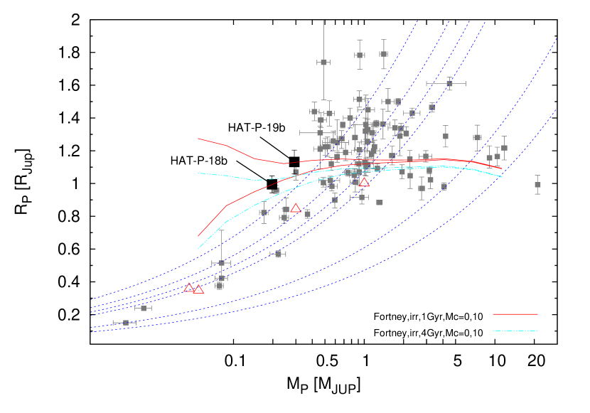
Figure 10.— Mass–radius diagram of known TEPs (small filled squares). HAT-P-18b and HAT-P-19b are shown as large filled squares. Overlaid are Fortney et al. (2007) planetary isochrones interpolated to the solar equivalent semi-major axis of HAT-P-18b for ages of 1.0 Gyr (upper, solid lines) and 4 Gyr (lower dashed-dotted lines) and core masses of 0 and 10 $M_{\earth}$(upper and lower lines respectively), as well as isodensity lines for 0.4, 0.7, 1.0, 1.33, 5.5 and 11.9$\rm g\,cm^{-3}$(dashed lines). Solar system planets are shown with open triangles.

Figure 10 compares HAT-P-18b and HAT-P-19b to other known TEPs on a mass-radius diagram. We discuss the properties of each planet in turn.

4.1. HAT-P-18b

From the Fortney et al. (2007) planetary models, the expected radius for a coreless $0.20\pm 0.01$ $M_{\rm J}$ planet orbiting a 4.5 Gyr star with a Solar-equivalent semi-major axis of $0.1073\pm 0.0071$ AU is $\sim 1.02$ $R_{\rm J}$, which is consistent with the measured radius for HAT-P-18b of $1.00\pm 0.05$ $R_{\rm J}$. The preferred age for HAT-P-18 from the YY isochrones ($12.4_{-6.4}^{+4.4}$ Gyr), is somewhat older than 4.5 Gyr, in which case the expected planetary radius would be even smaller. If a slight core of $10$ $M_{\earth}$ is assumed, the expected radius of $0.91$ $R_{\rm J}$ is below the measured radius. We conclude therefore that HAT-P-18b is a predominately hydrogen-helium gas giant planet, and does not possess a significant heavy element core.

HAT-P-18b is perhaps most similar in properties to the slightly higher density planet HAT-P-12b ($M=0.211\pm 0.012$ $M_{\rm J}$, $R=0.959_{-0.021}^{+0.029}$ $R_{\rm J}$; Hartman et al., 2009). Both planets orbit K dwarfs (HAT-P-18 has mass $M_{\star}=0.77\pm 0.03$ $M_{\sun}$, and HAT-P-12 has mass $M_{\star}=0.73\pm 0.02$ $M_{\sun}$). However HAT-P-18 appears to be older than HAT-P-12, having an isochrone age of $12.4_{-6.4}^{+4.4}$ Gyr compared with $2.5\pm 2.0$ Gyr for HAT-P-12. HAT-P-18 is also more metal rich ([Fe/H]=$+0.10\pm 0.08$) than HAT-P-12 ([Fe/H]=$-0.36\pm 0.04$).

4.2. HAT-P-19b

Like HAT-P-18b, HAT-P-19b also does not appear to possess a signficant heavy element core. From the Fortney et al. (2007) planetary models, the expected radius for a coreless $0.29\pm 0.02$ $M_{\rm J}$ planet orbiting a 4.5 Gyr star with a Solar-equivalent semi-major axis of $0.0763\pm 0.0065$ AU is $\sim 1.02$ $R_{\rm J}$, which is lower than the measured radius for HAT-P-19b of $1.13\pm 0.07$ $R_{\rm J}$. If an age of 1.0 Gyr is assumed, the expected planet radius increases to 1.06 $R_{\rm J}$, but is still slightly lower than, though consistent with, the measured radius.

Like HAT-P-18b, HAT-P-19b is also very similar in mass/radius to another TEP, in this case WASP-21b ($M=0.30\pm 0.01$ $M_{\rm J}$, $R=1.07\pm 0.05$ $R_{\rm J}$; Bouchy et al., 2010). WASP-21b orbits a somewhat hotter star than HAT-P-19b (WASP-21 has $M=1.01_{-0.025}^{+0.024}$ $M_{\sun}$, while HAT-P-19 has $M=0.84\pm 0.04$ $M_{\sun}$). HAT-P-19 is also more metal rich than WASP-21 ([Fe/H]=$+0.23\pm 0.08$ for HAT-P-19, while [Fe/H]=$-0.4\pm 0.1$ for WASP-21).

As noted in Section 3.3, the RV residuals of HAT-P-19 show a linear trend in time, which is evidence for a third body in the system. The evidence for this trend comes entirely from the Keck/HIRES observations which span 144 days. Although the Subaru/HDS observations predate the Keck/HIRES observations, the uncertain RV zero-point difference between these two datasets prevents us from comparing the Subaru/HDS observations with the Keck/HIRES observations to extend the baseline for measuring the linear variation in the RV residuals. The Subaru/HDS observations span only 3 days, so the trend is not evident in this dataset. Following Winn et al. (2010), we set $\dot{\gamma}\sim GM_{c}\sin i_{c}/a_{c}^{2}$ to give an order-of-magnitude constraint on the third body, assuming the orbit is circular. This gives

$$\left(\frac{M_{c}\sin i_{c}}{M_{\rm J}}\right)\left(\frac{a_{c}}{1AU}\right)^{-2}\sim 0.9$$ (2)

The time span of the RV measurements, and the lack of evidence for jerk ($\ddot{\gamma}$) in the RV residuals, lets us put a rough limit on the third body’s orbital period of $P_{c}\gtrsim 2\times 144=288$ d, or $a_{c}\gtrsim 0.8$ AU. This gives a rough lower limit on the mass of the third body of $M_{c}\gtrsim 0.6$ $M_{\rm J}$, though this depends on the eccentricity, argument of periastron, and time of conjunction. The object could also be a low-mass star with $M>90$ $M_{\rm J}$ if it has $a_{c}\gtrsim 10$ AU.

4.3. Core Mass–Metallicity Correlation

As noted in the introduction, the previously known Saturn-mass planets exhibited a suggestive correlation between core mass (or density) and host star metallicity. The two low density planets HAT-P-12b and WASP-21b are consistent with having no core, and orbit sub-solar metallicity stars. While the higher density planets Kepler-9b, Kepler-9c, CoRoT-8b, WASP-29b, and HD 149026b are consistent with having substantial cores, and orbit super-solar metallicity stars. The apparent correlation between planet core mass and host star metallicity was previously noted by Guillot et al. (2006) and Burrows et al. (2007) for all TEPs known at the time (nine and fourteen respectively). Many of the planets with $M\gtrsim 0.4$ $M_{\rm J}$ have radii that are larger than can be accommodated by theoretical models, so it is unclear whether the inferred core masses are physically meaningful for these planets. Nonetheless, for planets in the mass-range $0.4$–$0.7$ $M_{\rm J}$ Enoch et al. (2010) find that planet radius is inversely proportional to host star metallicity, which is what would be expected if the heavy element content of these planets (or core mass) is proportional to host star metallicity. Figure 11 shows the relation between core mass inferred from the Fortney et al. (2007) models and stellar metallicity for planets with $0.15<M<0.4$ $M_{\rm J}$, and $0.4<M<0.6$ $M_{\rm J}$. HAT-P-18b and HAT-P-19b do not follow the correlation that was previously seen for the other Saturn-mass planets. However, since the sample size of known Saturn-mass TEPs is still quite small, further discoveries are needed to illuminate the properties of planets in this mass-range.

Figure 11.— Planet core mass vs. host star metallicity for planets with $0.15<M<0.4$ $M_{\rm J}$ (left) and $0.4<M<0.6$ $M_{\rm J}$ (right). The core mass for each planet is determined by linear interpolation within the Fortney et al. (2007) planet model tables for the estimated age, mass, and solar-equivalent semimajor axis of the planet. We adopt an age of $4.0$ Gyr or $0.3$ Gyr for systems with an estimated age greater or less than these limits, and we adopt a solar-equivalent semimajor axis of $9.5$ AU for Saturn. Planets with a negative inferred core mass have radii that are too large to be accommodated by the Fortney et al. (2007) models. In this case the core mass is linearly extrapolated from the models, and provides a measure for the degree to which the observed radius disagrees with the models. The location of Saturn is indicated by the “S” in the left plot. HAT-P-18b and HAT-P-19b do not follow the previously suggestive correlation between core mass and host star metallicity for Saturn-mass planets. No correlation is apparent for planets with $M>0.6$ $M_{\rm J}$.

References

- Alibert et al. (2005) Alibert, Y., Mordasini, C., Benz, W., & Winisdoerffer, C. 2005, A&A, 434, 343
- Bakos et al. (2004) Bakos, G. Á., Noyes, R. W., Kovács, G., Stanek, K. Z., Sasselov, D. D., & Domsa, I. 2004, PASP, 116, 266
- Bakos et al. (2007) Bakos, G. Á., et al. 2007, ApJ, 670, 826
- Bakos et al. (2010) Bakos, G. Á., et al. 2010, ApJ, 710, 1724
- Baraffe et al. (1998) Baraffe, I., Chabrier, G., Allard, F., & Hauschildt, P. H. 1998, A&A, 337, 403
- Bordé et al. (2010) Bordé, P., et al. 2010, A&A, in press, arXiv:1008.0325
- Bouchy et al. (2010) Bouchy, F., et al. 2010, A&A, 519, 98
- Buchhave et al. (2010) Buchhave, L. A., et al. 2010, ApJ, 720, 1118
- Burrows et al. (2007) Burrows, A., Hubeny, I., Budaj, J., & Hubbard, W. B. 2007, ApJ, 661, 502
- Butler et al. (1996) Butler, R. P. et al. 1996, PASP, 108, 500
- Cabrera et al. (2010) Cabrera, J., et al. 2010, A&A, submitted
- Carpenter (2001) Carpenter, J. M. 2001, AJ, 121, 2851
- Carter et al. (2009) Carter, J. A., Winn, J. N., Gilliland, R., & Holman, M. J. 2009, ApJ, 696, 241
- Charbonneau (2009) Charbonneau, D. 2009, in “Transiting Planets, Proceedings of the International Astronomical Union, IAU Symposium, Volume 253”, eds. F. Pont, D. Sasselov, & M. Holman, (Cambridge: Cambridge), p. 1
- Claret (2004) Claret, A. 2004, A&A, 428, 1001
- Djupvik & Andersen (2010) Djupvik, A. A., & Andersen, J. 2010, in “Highlights of Spanish Astrophysics V” eds. J. M. Diego, L. J. Goicoechea, J. I. González-Serrano, & J. Gorgas (Springer: Berlin), p. 211
- Droege et al. (2006) Droege, T. F., Richmond, M. W., & Sallman, M. 2006, PASP, 118, 1666
- Enoch et al. (2010) Enoch, B., et al. 2010, MNRAS, submitted. arXiv:1009.5917
- Etzel (1981) Etzel, P. B. 1981, NATO ASI, p. 111
- Frandsen & Lindberg (1999) Frandsen, S., & Lindberg, B. 1999, in “Astrophysics with the NOT”, eds. H. Karttunen, & V. Piirola, (Piikkio, Finland: University of Turku, Tuorla Observatory), p. 71
- Ford (2006) Ford, E. 2006, ApJ, 642, 505
- Fortney et al. (2007) Fortney, J. J., Marley, M. S., & Barnes, J. W. 2007, ApJ, 659, 1661
- Füresz, G. (2008) Füresz, G. 2008, Ph.D. thesis, University of Szeged, Hungary
- Girardi et al. (2000) Girardi, L., Bressan, A., Bertelli, G., & Chiosi, C. 2000, A&AS, 141, 371
- Gray (1992) Gray, D. F. 1992, Camb. Astrophys. Ser., Vol. 20,
- Guillot et al. (2006) Guillot, T., Santos, N. C., Pont, F., Iron, N., Melo, C., & Ribas, I. 2006, A&A, 453, L21
- Hartman et al. (2009) Hartman, J. D., et al. 2009, ApJ, 706, 785
- Hansen & Barman (2007) Hansen, B. M. S., & Barman, T. 2007, ApJ, 671, 861
- Hebb et al. (2009) Hebb, L., et al. 2009, ApJ, 693, 1920
- Hellier et al. (2010) Hellier, C., et al. 2010, ApJ, submitted, arXiv:1009.5318
- Holman et al. (2010) Holman, M. J., et al. 2010, Science, 330, 51
- Kovács et al. (2002) Kovács, G., Zucker, S., & Mazeh, T. 2002, A&A, 391, 369
- Kovács et al. (2005) Kovács, G., Bakos, G. Á., & Noyes, R. W. 2005, MNRAS, 356, 557
- Kovács et al. (2010) Kovács, G., et al. 2010, ApJ submitted, arXiv:1005.5300
- Latham (1992) Latham, D. W. 1992, in IAU Coll. 135, Complementary Approaches to Double and Multiple Star Research, ASP Conf. Ser. 32, eds. H. A. McAlister & W. I. Hartkopf (San Francisco: ASP), 110
- Mandel & Agol (2002) Mandel, K., & Agol, E. 2002, ApJ, 580, L171
- Marcy & Butler (1992) Marcy, G. W., & Butler, R. P. 1992, PASP, 104, 270
- Nelson & Davis (1972) Nelson, B., & Davis, W. D. 1972, ApJ, 174, 617
- Noguchi et al. (2002) Noguchi, N., et al. 2002, PASJ, 54, 819
- Pál & Bakos (2006) Pál, A., & Bakos, G. Á. 2006, PASP, 118, 1474
- Pál et al. (2008) Pál, A., et al. 2008, ApJ, 680, 1450
- Pál (2009) Pál, A. 2009, MNRAS, 396, 1737
- Pál (2009b) Pál, A. 2009b, arXiv:0906.3486, PhD thesis
- Popper & Etzel (1981) Popper, D. M., & Etzel, P. B. 1981, AJ, 86, 102
- Press et al. (1992) Press, W. H., Teukolsky, S. A., Vetterling, W. T. & Flannery, B. P., 1992, Numerical Recipes in C: the art of scientific computing, Second Edition, Cambridge University Press
- Sato et al. (2002) Sato, B., et al. 2002, PASJ, 54, 873
- Sato et al. (2005) Sato, B., et al. 2005, ApJ, 633, 465
- Skrutskie et al. (2006) Skrutskie, M. F., et al. 2006, AJ, 131, 1163
- Southworth et al. (2004a) Southworth, J., Maxted, P. F. L., & Smalley, B. 2004a, MNRAS, 351, 1277
- Southworth et al. (2004b) Southworth, J., Zucker, S., Maxted, P. F. L., & Smalley, B. 2004b, MNRAS, 355, 986
- Sozzetti et al. (2007) Sozzetti, A. et al. 2007, ApJ, 664, 1190
- Standish (1995) Standish, E. M. 1995, Highlights Astron., 10, 180
- Tingley & Sackett (2005) Tingley, B., & Sackett, P. D. 2005, ApJ, 627, 1011
- Torres et al. (2002) Torres, G., Neuhäuser, R., & Guenther, E. W. 2002, AJ, 123, 701
- Torres et al. (2005) Torres, G., Konacki, M., Sasselov, D. D., & Jha, S. 2005, ApJ, 619, 558
- Torres et al. (2007) Torres, G. et al. 2007, ApJ, 666, 121
- Valenti & Fischer (2005) Valenti, J. A., & Fischer, D. A. 2005, ApJS, 159, 141
- Valenti & Piskunov (1996) Valenti, J. A., & Piskunov, N. 1996, A&AS, 118, 595
- Vogt et al. (1994) Vogt, S. S. et al. 1994, Proc. SPIE, 2198, 362
- Vaughan, Preston & Wilson (1978) Vaughan, A. H., Preston, G. W., & Wilson, O. C. 1978, PASP, 90, 267
- Winn et al. (2010) Winn, J. N., et al. 2010, ApJ, 718, 575
- Yi et al. (2001) Yi, S. K. et al. 2001, ApJS, 136, 417