Extremal Charged Rotating Dilaton Black Holes
in Odd Dimensions

Abstract

Employing higher order perturbation theory, we find a new class of charged rotating black hole solutions of Einstein-Maxwell-dilaton theory with general dilaton coupling constant. Starting from the Myers-Perry solutions, we use the electric charge as the perturbative parameter, and focus on extremal black holes with equal-magnitude angular momenta in odd dimensions. We perform the perturbations up to 4th order for black holes in 5 dimensions and up to 3rd order in higher odd dimensions. We calculate the physical properties of these black holes and study their dependence on the charge and the dilaton coupling constant.

I Introduction

Starting with the pioneering work of Kaluza and Klein, the quest to unify the fundamental forces of nature has led to higher dimensional theories, yielding additional fields upon reduction to lower dimensions. In the low energy limit of the string theory, one recovers for instance, Einstein gravity along with a scalar dilaton field which is non-minimally coupled to matter fields Green:1987sp .

Exact solutions for charged dilaton black holes where the dilaton is coupled to the Maxwell field have been considered by many authors. This showed that the presence of the dilaton has important consequences for the black hole properties. Gibbons and Maeda, for instance, obtained the general family of static charged dilaton black holes in $D$ dimensions Gibbons:1987ps ; Garfinkle:1990qj ; Gregory:1992kr . They demonstrated that the physical properties of the black holes depend sensitively on the value of the dilaton coupling constant, with critical values of this coupling constant separating qualitatively different thermodynamical behaviour.

Exact rotating dilaton black hole solutions have been obtained only for special values of the dilaton coupling constant. In 4 dimensions, rotating charged dilaton black holes are known for the Kaluza-Klein value of the coupling constant, where solution generating techniques can be applied Frolov:1987rj ; Rasheed:1995zv ; Larsen:1999pp . For general dilaton coupling constant, only perturbative results for small angular momentum Horne:1992zy ; Shiraishi:1992jt or small charge Casadio:1996sj are available Horne:1992zy ; Casadio:1996sj as well as numerical results Kleihaus:2003df . Interestingly, already a small amount of rotation leads to a qualitative change of the properties of extremal black holes. Moreover, the presence of both electric and magnetic charge allows for rotating black holes with static Rasheed:1995zv and counterrotating horizons Kleihaus:2003df .

In higher dimensions, the charged dilatonic generalizations of the Myers-Perry black holes Myers:1986un are known for the respective Kaluza-Klein value of the dilaton coupling constant, which depends on the number of dimensions $D$. Their domain of existence and their properties were discussed in Kunz:2006jd . The inclusion of additional fields, as required by supersymmetry or string theory, led to further exact solutions of higher dimensional rotating dilatonic black holes Youm:1997hw ; Llatas:1996gh ; Horowitz:1995tm .

Generalizing the lowest order perturbative Einstein-Maxwell results for higher-dimensional charged rotating black holes Aliev:2005npa ; Aliev:2006yk to the case of Einstein-Maxwell-dilaton theory with general dilaton coupling constant, the properties of charged rotating dilaton black holes with infinitesimally small angular momentum were investigated in Sheykhi:2008bs . Also charged rotating dilaton black rings were constructed perturbatively Kunduri:2004da . Rotating dilatonic black holes with the charge as the perturbative parameter have not yet been obtained for general dilaton coupling.

In general, rotating black holes in $D$ dimensions possess $[(D-1)/2]$ independent angular momenta Myers:1986un . When specializing to black holes with equal-magnitude angular momenta in odd dimensions, however, the symmetry of the solutions enhances greatly. This reduces the problem from cohomogeneity-$[(D-1)/2]$ to cohomogeneity-1, and thus makes the solutions amenable to higher order perturbative techniques.

Recently, employing higher order perturbation theory with the charge as the perturbative parameter, the properties of such cohomogeneity-1 rotating Einstein-Maxwell black holes were investigated in five dimensions NavarroLerida:2007ez . Subsequently, this perturbative method was extended to obtain Einstein-Maxwell black holes with equal-magnitude angular momenta in general odd dimensions, focussing on extremal black holes Allahverdizadeh:2010xx .

These higher order perturbative results confirmed previous numerical studies Kunz:2005nm ; Kunz:2006eh , showing that the lowest order perturbative results for the gyromagnetic ratio, $g=D-2$ Aliev:2004ec ; Aliev:2005npa ; Aliev:2006yk receive corrections, depending upon the charge to mass ratio $Q/M$. Indeed, in 3rd order the gyromagnetic ratio becomes $g=(D-2)\left[1+\frac{1}{16}\left(\frac{Q}{M}\right)^{2}\right]$ Allahverdizadeh:2010xx . The higher order perturbative method was also employed to study cohomogeneity-1 black holes in Einstein-Maxwell-Chern-Simons theory Allahverdizadeh:2010xx , allowing for further insight into these intriguing black holes Breckenridge:1996sn ; Breckenridge:1996is ; Cvetic:2004hs ; Chong:2005hr ; Kunz:2005ei ; Kunz:2006yp ; Aliev:2008bh .

The symmetry enhancement for black holes in odd dimensions with equal-magnitude angular momenta is retained in the presence of a dilaton field. In this paper we are thus led to apply the higher order perturbative method to find charged rotating black holes in dilaton gravity. Again, we focus on black holes at extremality. Starting from the Myers-Perry black holes, we evaluate the perturbative series up to 4th order in the charge for black holes in 5 dimensions, and up to 3rd order for black holes in more than 5 dimensions. We determine the physical properties of these black holes for general dilaton coupling constant. In particular, we investigate the effects of the presence of the dilaton field and the perturbative parameter on the gyromagnetic ratio of these rotating black holes.

The remainder of this paper is outlined as follows. In the next section, we present the metric, the dilaton field and the gauge potential for black holes in odd dimensions with equal-magnitude angular momenta. We introduce the perturbation series and present the global and horizon properties for these black holes. In section III we give the perturbative solution for extremal black holes of Einstein-Maxwell-dilaton theory in 5 dimensions. In section IV we present the generalization to general odd dimensions. We demonstrate the effect of the presence of the dilaton field and the charge on the mass, the angular momentum, the magnetic moment and the gyromagnetic ratio of these extremal rotating black holes. We also evaluate their horizon properties. Our conclusions are drawn in section V. The formulae for the metric, the dilaton field and the gauge potential in $D$ dimensions are given in the Appendix.

II Black hole properties

II.1 Einstein-Maxwell dilaton theory

We consider Einstein-Maxwell dilaton theory in $D$ dimensions, possessing the action

$$S = \int d^{D}x\sqrt{-g}\left(R\text{ }-\frac{1}{2}\partial_{\mu}\Phi\partial^{\mu}\Phi-\frac{1}{4}e^{-2h\Phi}F_{\mu\nu}F^{\mu\nu}\right),$$ (1)

where ${R}$ is the scalar curvature, $\Phi$ is the dilaton field, $F_{\mu\nu}=\partial_{\mu}A_{\nu}-\partial_{\nu}A_{\mu}$ is the electromagnetic field tensor, and $A_{\mu}$ is the electromagnetic potential. $h$ is an arbitrary constant governing the strength of the coupling between the dilaton and the Maxwell field. The units are chosen such that $16\pi G_{D}=1$.

The equations of motion can be obtained by varying the action with respect to the metric $g_{\mu\nu}$, the dilaton field $\Phi$ and the gauge potential $A_{\mu}$, yielding

$$G_{\mu\nu}=\frac{1}{2}\left[\partial_{\mu}\Phi\partial_{\nu}\Phi-\frac{1}{2}g_{\mu\nu}\partial_{\rho}\Phi\partial^{\rho}\Phi+e^{-2h\Phi}\left(F_{\mu\rho}{F_{\nu}}^{\rho}-\frac{1}{4}g_{\mu\nu}F_{\rho\sigma}F^{\rho\sigma}\right)\right]\ ,$$ (2)

$$\nabla^{2}\Phi=-\frac{h}{2}e^{-2h\Phi}F_{\mu\nu}F^{\mu\nu}\ ,$$ (3)

$$\nabla_{\mu}\left(e^{-2h\Phi}F^{\mu\nu}\right)=0\ .\$$ (4)

II.2 Black holes in odd dimensions

In general, stationary black holes in $D$ dimensions possess $N=[(D-1)/2]$ independent angular momenta $J_{i}$ associated with $N$ orthogonal planes of rotation Myers:1986un . ($[(D-1)/2]$ denotes the integer part of $(D-1)/2$, corresponding to the rank of the rotation group $SO(D-1)$.) The general black holes solutions then fall into two classes, into even-$D$ and odd-$D$-solutions Myers:1986un . Here we focus on perturbative charged rotating black holes in odd dimensions.

When all $N$ angular momenta have equal-magnitude, the symmetry of the Myers-Perry black holes is strongly enhanced. In odd dimensions, the symmetry then increases from $R\times U(1)^{N}$ to $R\times U(N)$, thus changing the problem from cohomogeneity-$N$ to cohomogeneity-1. The original system of partial differential equations in $N$ variables then reduces to a system of ordinary differential equations. In the presence of an electromagnetic field, this symmetry enhancement is retained Kunz:2006eh , and likewise in the presence of a dilaton field. Since the angular dependence factorizes, the rotating cohomogeneity-1 black holes of Einstein-Maxwell-dilaton theory are amenable to higher order perturbation theory, as developed recently NavarroLerida:2007ez ; Allahverdizadeh:2010xx for Einstein-Maxwell and Einstein-Maxwell-Chern-Simons theory.

To obtain such perturbative charged dilatonic generalizations of the $D$-dimensional Myers-Perry solutions Myers:1986un , we employ the following parametrization for the metric Kunz:2006eh ; Kunz:2006yp

$$ds^{2} = g_{tt}dt^{2}+\frac{dr^{2}}{W}+r^{2}\left[\sum^{N-1}_{i=1}\left(\prod^{i-1}_{j=0}\cos^{2}\theta_{j}\right)d\theta^{2}_{i}+\sum^{N}_{k=1}\left(\prod^{k-1}_{l=0}\cos^{2}\theta_{l}\right)\sin^{2}\theta_{k}d\varphi^{2}_{k}\right]$$

$$+ V\left[\sum^{N}_{k=1}\left(\prod^{k-1}_{l=0}\cos^{2}\theta_{l}\right)\sin^{2}\theta_{k}\varepsilon_{k}d\varphi_{k}\right]^{2}-2B\sum^{N}_{k=1}\left(\prod^{k-1}_{l=0}\cos^{2}\theta_{l}\right)\sin^{2}\theta_{k}\varepsilon_{k}d\varphi_{k}dt\ ,\phantom{a=a}$$

where $\theta_{0}\equiv 0$, $\theta_{i}\in[0,\pi/2]$ for $i=1,...,N-1$, $\theta_{N}\equiv\pi/2$, $\varphi_{k}\in[0,2\pi]$ for $k=1,...,N$, and $\varepsilon_{k}=\pm 1$ denotes the sense of rotation in the $k$-th orthogonal plane of rotation. An adequate parametrization for the gauge potential is given by

$$A_{\mu}dx^{\mu} = a_{t}dt+a_{\varphi}\sum^{N}_{k=1}\left(\prod^{k-1}_{l=0}\cos^{2}\theta_{l}\right)\sin^{2}\theta_{k}\varepsilon_{k}d\varphi_{k}\ ,$$ (6)

where the metric functions $g_{tt}$, $W$, $V$, $B$, the functions for the gauge potential $a_{t}$, $a_{\varphi}$, and the dilaton function $\Phi$ depend only on the radial coordinate $r$.

II.3 Perturbation theory

We now consider perturbations about the Myers-Perry solutions, with the electric charge as the perturbative parameter. In the presence of the dilaton field we obtain the perturbation series in the general form

$$g_{tt}=-1+\frac{2\hat{M}}{r^{D-3}}+q^{2}g^{(2)}_{tt}+q^{4}g^{(4)}_{tt}+O(q^{6})\ ,$$ (7)

$$W=1-\frac{2\hat{M}}{r^{D-3}}+\frac{2\hat{J}^{2}}{\hat{M}r^{D-1}}+q^{2}W^{(2)}+q^{4}W^{(4)}+O(q^{6})\ ,$$ (8)

$$V=\frac{2\hat{J}^{2}}{\hat{M}r^{D-3}}+q^{2}V^{(2)}+q^{4}V^{(4)}+O(q^{6})\ ,$$ (9)

$$B=\frac{2\hat{J}}{r^{D-3}}+q^{2}B^{(2)}+q^{4}B^{(4)}+O(q^{6})\ ,$$ (10)

$$\Phi=q^{2}\Phi^{(2)}+q^{4}\Phi^{(4)}+O(q^{6})\ ,$$ (11)

$$a_{t}=qa^{(1)}_{t}+q^{3}a^{(3)}_{t}+O(q^{5})\ ,$$ (12)

$$a_{\varphi}=qa^{(1)}_{\varphi}+q^{3}a^{(3)}_{\varphi}+O(q^{5})\ ,$$ (13)

where $q$ is the perturbative parameter associated with the electric charge (see Eq. (IV) below). Because of charge reversal symmetry the perturbations contain only even powers of $q$ in the metric and the dilaton, and only odd powers of $q$ in the gauge potential.

Inserting the metric Eq. (II.2) and the gauge potential Eq. (6) with the perturbation expansion Eqs. (7-13) into the field equations Eqs. (2-4), we then solve these equations order by order.

II.4 Physical Quantities

The mass $M$, the equal-magnitude angular momenta $|J_{i}|=J$, the dilaton charge $\Sigma$, the electric charge $Q$, and the magnetic moments $\mu_{\rm mag}$ can be read off the asymptotic behavior of the metric, the dilaton function, and the gauge potential Kunz:2006eh ; Kunz:2006yp

$$g_{tt}=-1+\frac{\tilde{M}}{r^{D-3}}+...\ ,\quad B=\frac{\tilde{J}}{r^{D-3}}+...\ ,\quad\Phi=\frac{\tilde{\Sigma}}{r^{D-3}}+...\ ,$$

$$a_{t}=\frac{\tilde{Q}}{r^{D-3}}+...\ ,\quad a_{\varphi}=\frac{\tilde{\mu}_{\rm mag}}{r^{D-3}}+...\ ,$$ (14)

where

$$\tilde{M} = \frac{1}{(D-2)A(S^{D-2})}M\ ,$$

$$\tilde{J} = \frac{1}{2A(S^{D-2})}J\ ,$$

$$\tilde{\Sigma} = \frac{1}{(D-3)A(S^{D-2})}\Sigma\ ,$$

$$\tilde{Q} = \frac{1}{(D-3)A(S^{D-2})}Q\ ,$$

$$\tilde{\mu}_{\rm mag} = \frac{1}{(D-3)A(S^{D-2})}\mu_{\rm mag}\ ,$$ (15)

and $A(S^{D-2})$ is the area of the unit $(D-2)$-sphere. The definition of the magnetic moment is gauge-invariant and refers to an asymptotic rest frame Aliev:2004ec ; Allahverdizadeh:2010xx . The gyromagnetic ratio $g$ is given by

$$g=\frac{2M\mu_{\rm mag}}{QJ}\ .$$ (16)

The event horizon is located at $r=r_{\rm H}$. The horizon angular velocities $|\Omega_{i}|=\Omega$ can be defined by imposing the Killing vector field

$$\chi=\xi+\Omega\sum^{N}_{k=1}\epsilon_{k}\eta_{k}\ ,$$ (17)

to be null on and orthogonal to the horizon ($\chi=\partial_{t}$ and $\eta_{k}=\partial_{\varphi_{k}}$). The horizon electrostatic potential $\Psi_{\rm el,H}$ of these black holes is given by

$$\Psi_{\rm el,H}=\left.(a_{t}+\Omega a_{\varphi})\right|_{r=r_{\rm H}}\ ,$$ (18)

and the surface gravity $\kappa_{\rm sg}$ is defined by

$$\kappa^{2}_{\rm sg}=\left.-\frac{1}{2}(\nabla_{\mu}\chi_{\nu})(\nabla^{\mu}\chi^{\nu})\right|_{r=r_{\rm H}}\ .$$ (19)

The black holes further satisfy the Smarr-like mass formula Kleihaus:2002tc ; Kleihaus:2003df ; Kunz:2006jd

$$M=2\frac{D-2}{D-3}{\kappa_{\rm sg}A_{\rm H}}+\frac{D-2}{D-3}N\Omega J+2\Psi_{\rm el,H}Q+\frac{\Sigma}{h}\ .$$ (20)

With the relation

$$\frac{\Sigma}{h}=-\Psi_{\rm el,H}Q\ ,$$ (21)

the Smarr mass formula can be given its usual form Gauntlett:1998fz

$$M=2\frac{D-2}{D-3}{\kappa_{\rm sg}A_{\rm H}}+\frac{D-2}{D-3}N\Omega J+\Psi_{\rm el,H}Q\ .$$ (22)

Since the relations Eq. (21) and  (22) must also hold for the perturbation solutions, this provides a good check of consistency for the perturbative scheme.

III Charged dilaton black holes in 5 dimensions

Here we first present the perturbative solutions, obtained in 4th order in the charge, for extremal black holes with equal-magnitude angular momenta in Einstein-Maxwell-dilaton theory for general dilaton coupling constant $h$.

We now perform perturbation theory in the charge to 4th order. We impose the extremality condition on the black holes and fix the angular momentum $J$ for all orders. We further impose a regularity condition at the horizon. This choice then fixes all integration constants which appear in the scheme.

Introducing the parameter $\nu$ for the extremal Myers-Perry solutions by

$${\hat{M}}=2\nu^{2},\quad\quad{\hat{J}}=2\nu^{3},$$ (23)

we obtain for the metric and the dilaton field the perturbation expansion up to 5th order in the perturbative parameter $q$ and for the gauge potential functions up to 4th order

$$g_{tt} = -1+\frac{4\nu^{2}}{r^{2}}+\frac{r^{2}-4\nu^{2}}{12\nu^{2}r^{4}}q^{2}$$

$$+\left[\frac{(2-3h^{2})(r^{2}-2\nu^{2})^{2}}{216\nu^{8}r^{4}}\ln\left(1-\frac{2\nu^{2}}{r^{2}}\right)+\frac{(11-18h^{2})\nu^{2}r^{4}-16(2-3h^{2})\nu^{4}r^{2}+16\nu^{6}}{576\nu^{8}r^{6}}\right]q^{4}$$

$$+O(q^{6})\ ,$$

$$W = 1-\frac{4\nu^{2}}{r^{2}}+\frac{4\nu^{4}}{r^{4}}-\frac{r^{2}-2\nu^{2}}{12\nu^{2}r^{4}}q^{2}+\Bigg{\{}\frac{(2-3h^{2})(r^{2}-2\nu^{2})^{3}}{288\nu^{10}r^{4}}\ln\left(1-\frac{2\nu^{2}}{r^{2}}\right)$$

$$+\frac{12(2-3h^{2})r^{8}-(121-186h^{2})\nu^{2}r^{6}+(181-204h^{2})\nu^{4}r^{4}-8(8-15h^{2})\nu^{6}r^{2}+144h^{2}\nu^{8}}{1728\nu^{8}r^{8}}\Bigg{\}}q^{4}$$

$$+O(q^{6})\ ,$$

$$V = \frac{4\nu^{4}}{r^{2}}-\frac{(r^{2}+2\nu^{2})}{6r^{4}}q^{2}-\Bigg{\{}\frac{(2-3h^{2})(r^{2}-2\nu^{2})(3r^{6}+8\nu^{6})}{864\nu^{10}r^{4}}\ln\left(1-\frac{2\nu^{2}}{r^{2}}\right)$$

$$+\frac{4(2-3h^{2})r^{8}-4(2-3h^{2})\nu^{2}r^{6}-7\nu^{4}r^{4}+16(1-3h^{2})\nu^{6}r^{2}-16\nu^{8}}{576\nu^{8}r^{6}}\Bigg{\}}q^{4}+O(q^{6})\ ,$$

$$B = \frac{4\nu^{3}}{r^{2}}-\frac{\nu}{3r^{4}}q^{2}-\Bigg{\{}\frac{(2-3h^{2})(r^{2}-2\nu^{2})(3r^{4}-6\nu^{2}r^{2}+16\nu^{4})}{1728\nu^{9}r^{4}}\ln\left(1-\frac{2\nu^{2}}{r^{2}}\right)$$

$$+\frac{(2-3h^{2})r^{6}-3(2-3h^{2})\nu^{2}r^{4}+3(4-8h^{2})\nu^{4}r^{2}-8\nu^{6}}{288\nu^{7}r^{6}}\Bigg{\}}q^{4}+O(q^{6})\ ,$$

$$\Phi = \frac{-h}{4\nu^{2}r^{2}}q^{2}-\Bigg{\{}\frac{h(2-3h^{2})(r^{2}-2\nu^{2})}{144\nu^{8}r^{2}}\ln\left(1-\frac{2\nu^{2}}{r^{2}}\right)+\frac{((3-6h^{2})r^{2}-\nu^{2})h}{96\nu^{6}r^{4}}\Bigg{\}}q^{4}+O(q^{6})\ ,$$

$$a_{t} = \frac{1}{r^{2}}q+\Bigg{\{}\frac{(2-3h^{2})(r^{2}-2\nu^{2})}{72\nu^{6}r^{2}}\ln\left(1-\frac{2\nu^{2}}{r^{2}}\right)-\frac{(2+6h^{2})\nu^{2}-(2-3h^{2})r^{2}}{36\nu^{4}r^{4}}\Bigg{\}}q^{3}+O(q^{5})\ ,\ \ \ \$$

$$a_{\varphi} = -\frac{\nu}{r^{2}}q-\Bigg{\{}\frac{(2-3h^{2})(r^{4}-4\nu^{4})}{144\nu^{7}r^{2}}\ln\left(1-\frac{2\nu^{2}}{r^{2}}\right)$$ (24)

$$+\frac{(2-3h^{2})r^{4}+(1-6h^{2})\nu^{2}r^{2}-(4+12h^{2})\nu^{4}}{72\nu^{5}r^{4}}\Bigg{\}}q^{3}+O(q^{5})\ .$$

Clearly, for vanishing dilaton coupling constant, the previous results for rotating Einstein-Maxwell black holes are recovered NavarroLerida:2007ez .

We note, that for generic values of the dilaton coupling constant $h$ logarithms appear in the expansion. These logarithms disappear for the special value

$$h=h_{\rm KK}=\sqrt{\frac{2}{3}}\ .$$ (25)

This value precisely coincides with that value of the dilaton coupling, for which the exact general rotating black hole solutions are known Kunz:2006jd .

This situation is thus analogous to the case of Einstein-Maxwell-Chern-Simons theory Allahverdizadeh:2010xx , where the logarithms disappear, when the Chern-Simons coupling assumes its supergravity value, for which the exact general rotating black hole solutions are known Chong:2005hr . In fact, in both these special cases, the logarithms disappear at all orders.

From the above expansions the physical properties of the rotating dilaton black hole solutions can be extracted. To 4th order the global physical quantities are given by

$$M = 24\pi^{2}\nu^{2}+\frac{\pi^{2}}{2\nu^{2}}q^{2}+\frac{\pi^{2}(1-6h^{2})}{288\nu^{6}}q^{4}+O(q^{6})\ ,$$

$$J = 16\pi^{2}\nu^{3}\ (\mbox{for any order})\ ,$$

$$\Sigma = -\frac{\pi^{2}h}{\nu^{2}}q^{2}-\frac{\pi^{2}h(1-6h^{2})}{72\nu^{6}}q^{4}+O(q^{6})\ ,$$

$$Q = 4\pi^{2}q\ ,$$

$$\mu_{\rm{mag}} = 4\pi^{2}\nu q-\frac{\pi^{2}(1+3h^{2})}{18\nu^{3}}q^{3}+O(q^{5})\ ,$$ (26)

and the gyromagnetic ratio $g$ is given by

$$g=3+\frac{(1-6h^{2})}{48\nu^{4}}q^{2}+O(q^{4})\ .$$ (27)

Recently, it was shown that the presence of the dilaton field modifies the gyromagnetic ratio $g$, by applying lowest order perturbation theory with respect to the angular momentum and thus evaluating $g$ in the slowly rotating case Sheykhi:2008bs . Here, we can see that the dilaton field generically modifies the value of the gyromagnetic ratio in 2nd order in the charge, unless $h^{2}=h_{\rm cr}^{2}=1/6$. For $h<h_{\rm cr}$ the gyromagnetic ratio grows with increasing charge to mass ratio $Q/M$, whereas for $h>h_{\rm cr}$ it decreases with increasing $Q/M$, as seen in Fig. 1.

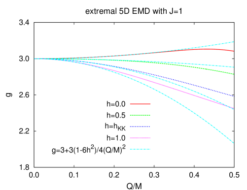
Figure 1: The 3rd order perturbative values for the gyromagnetic ratio $g$ versus the charge to mass ratio $Q/M$ for $D=5$ Einstein-Maxwell-dilaton black holes for several values of the dilaton coupling constant $h$ (cyan/dot-dashed). For comparison, the analytically known result ($h_{\rm KK}$) and exact numerical results ($h=0$, 0.5, 1.0) are also shown.

We compare in Fig. 1 the 3rd order perturbative results for the gyromagnetic ratio $g$ with the analytically known result for the Kaluza-Klein case ($h_{\rm KK}$) and numerical results for other values of the dilaton coupling constant ($h=0$, 0.5, 1.0). We note, that for small $h$ ($h=0$, 0.5) the perturbative results are rather good up to about one third of the domain of existence. Note, that the range of possible values of the charge to mass ratio $Q/M$ for these 5-dimensional black holes is bounded by $(Q/M)_{\rm max}$, where

$$\left(\frac{Q}{M}\right)_{\rm max}=\sqrt{\frac{1}{3}+h^{2}}\ .$$ (28)

For larger values of $h$ ($h_{\rm KK}$, 1.0) the range of validity of the 3rd order perturbative results decreases.

Let us now turn to the horizon properties of these black holes. Their event horizon is located at $r=r_{\rm H}$, where

$$r_{\rm H}=\sqrt{2}\nu+\frac{\sqrt{2}}{96\nu^{3}}q^{2}+\frac{\sqrt{2}(11-48h^{2})}{18432\nu^{7}}q^{4}+O(q^{6})\ .$$ (29)

The horizon angular velocity $\Omega$, the horizon area $A_{\rm H}$, and the horizon electrostatic potential $\Psi_{\rm el,H}$ are given by

$$\Omega=\frac{1}{2\nu}-\frac{1}{96\nu^{5}}q^{2}-\frac{(1-6h^{2})}{4608\nu^{9}}q^{4}+O(q^{6})\ ,$$

$$A_{\rm H}=8\pi^{2}\nu^{3}+O(q^{6})\ ,$$

$$\Psi_{\rm el,H}=\frac{1}{4\nu^{2}}q+\frac{(1-6h^{2})}{288\nu^{6}}q^{3}+O(q^{5})\ ,$$ (30)

and the surface gravity $\kappa_{\rm sg}$ vanishes for these extremal solutions.

IV Charged black holes in odd dimensions

To obtain the perturbative Einstein-Maxwell-dilaton black holes in the general case of $D$ odd dimensions, we proceed as in 5 dimensions. We fix the angular momentum for any perturbative order, and impose the extremality condition for all orders. We then introduce the parameter $\nu$ for the extremal Myers-Perry solutions in $D$ dimensions by

$$\hat{M}=\frac{(D-1)^{\frac{(D-1)}{2}}\nu^{D-3}}{4(D-3)^{\frac{(D-3)}{2}}}\ ,\quad\quad\hat{J}=\frac{(D-1)^{\frac{(D-1)}{2}}\nu^{D-2}}{4(D-3)^{\frac{(D-3)}{2}}}\ .$$ (31)

To fix all of the integration constants, we again need to make use of the regularity condition of the horizon. We employ the Smarr relation as a consistency check of the new perturbative black hole solutions.

The perturbative expansion for the metric, the dilaton field, and the gauge potential is exhibited in Appendix A for generic values of the dilaton coupling constant $h$. These expressions hold for the metric and the dilaton field in 3rd order, and for the gauge potential in 4th order. We note, that for generic values of $h$ the higher order expansions contain non-rational functions. As in 5 dimensions, however, the expansions simplify considerably when $h$ assumes the special dimension-dependent value

$$h_{\rm KK}=\frac{D-1}{\sqrt{2(D-1)(D-2)}}\ ,$$ (32)

for which the black hole solutions are known analytically Kunz:2006jd . Since the Einstein equations are modified by the presence of the dilaton in 4th order, the expansions for the metric functions given in the Appendix (namely, Eqs. (39-42)) do not depend on the dilaton coupling constant $h$. Concerning the dilaton field $\Phi$ the corresponding expression for the Kaluza-Klein solutions is nothing but Eq. (43) with $h$ restricted to Eq. (32). At the order of the perturbations we are treating in this paper, the main simplification for $h=h_{\rm KK}$ occurs for the gauge potential functions. The complicated integral expressions appearing in Eqs. (44-A) reduce to the following simple formulae for the Kaluza-Klein solutions:

$$a_{t} = \frac{q}{r^{D-3}}-\frac{1}{D-2}\left(\frac{D-3}{D-1}\right)^{\frac{D-3}{2}}\frac{1}{r^{2(D-3)}\nu^{D-3}}q^{3}+O(q^{5})\ ,$$ (33)

$$a_{\varphi} = -\frac{\nu q}{r^{D-3}}+\frac{(D-3)^{\frac{D-3}{2}}}{(D-2)(D-1)^{\frac{D-3}{2}}}\left[\frac{1}{r^{2(D-3)}\nu^{D-4}}+\frac{2(D-3)^{\frac{D-3}{2}}}{(D-1)^{\frac{D-1}{2}}}\frac{1}{r^{D-3}\nu^{2D-7}}\right]q^{3}$$ (34)

$$+O(q^{5})\ .$$

For a generic value of the dilaton coupling constant, by extracting the asymptotic behavior of the solutions Eqs. (39-45) from the perturbative expansion, we now obtain the global properties for these Einstein-Maxwell-dilaton black holes

$$M = A(S^{D-2})\left[\frac{\nu^{(D-3)}(D-2)(D-1)^{\frac{D-1}{2}}}{2(D-3)^{\frac{D-3}{2}}}+\frac{q^{2}(D-3)^{\frac{D-1}{2}}}{\nu^{D-3}(D-1)^{\frac{D-1}{2}}}\right]+O(q^{4})\ ,$$

$$J = \frac{A(S^{D-2})\nu^{D-2}(D-1)^{\frac{D-1}{2}}}{(D-3)^{\frac{D-3}{2}}}\ ,$$

$$\Sigma = -\frac{2A(S^{D-2})(D-3)^{\frac{D-1}{2}}h}{\nu^{D-3}(D-1)^{\frac{D-1}{2}}}q^{2}+O(q^{4})\ ,$$

$$Q = A(S^{D-2})(D-3)q\ ,$$

$$\mu_{\rm mag} = A(S^{D-2})(D-3)\left[q\nu-\frac{q^{3}(D-3)^{D-3}(D-3+2(D-2)h^{2})}{\nu^{2D-7}(D-2)^{2}(D-1)^{D-2}}\right]+O(q^{5})\ .$$ (35)

The dilaton charge $\Sigma$ is exhibited in Fig. 2 versus the charge to mass ratio $Q/M$ for Einstein-Maxwell-dilaton black holes in 5, 7 and 9 dimensions for the dilaton coupling constant $h_{\rm KK}$, where the solutions are known analytically Kunz:2006jd . Comparison shows, that the interval, where the 3rd order perturbative results are rather good, increases considerably with increasing dimension. (For the dilaton coupling constant $h_{\rm KK}$ the range of possible values of the charge to mass ratio $Q/M$ is bounded by $Q/M\leq 1$ in all dimensions.)

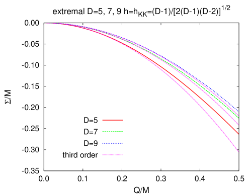
Figure 2: The 3rd order perturbative values for the dilaton charge $\Sigma$ versus the charge to mass ratio $Q/M$ for Einstein-Maxwell-dilaton black holes in 5, 7 and 9 dimensions for the dilaton coupling constant $h_{\rm KK}$ (purple/dotted). For comparison, the analytically known results are also shown.

The gyromagnetic ratio $g$, in particular, is given by

$$g=D-2+q^{2}\frac{(D-3)^{D-3}((D-3)^{2}-2(D-1)(D-2)h^{2})}{(D-2)(D-1)^{D-1}\nu^{2(D-3)}}+O(q^{4})\ .$$ (36)

Clearly, the gyromagnetic ratio of these fast rotating black holes is modified from its lowest order value $g=D-2$ in higher order perturbation theory, with appreciable contributions coming from the dilaton field (proportional to $h^{2}$). The gyromagnetic ratio is exhibited in Fig. 3 versus the charge to mass ratio $Q/M$ for Einstein-Maxwell-dilaton black holes in 5, 7 and 9 dimensions for the dilaton coupling constant $h_{\rm KK}$ and compared to the analytically known results Kunz:2006jd . As for the dilaton charge, we note that the 3rd order perturbative results are the better the higher the dimension.

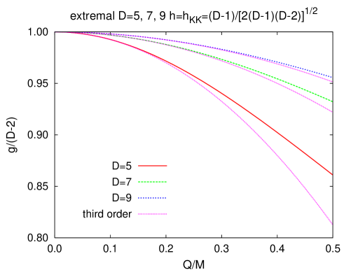
Figure 3: The 3rd order perturbative values for the gyromagnetic ratio $g$ versus the charge to mass ratio $Q/M$ for Einstein-Maxwell-dilaton black holes in 5, 7 and 9 dimensions for the dilaton coupling constant $h_{\rm KK}$ (purple/dotted). For comparison, the analytically known results are also shown.

The event horizon of these rotating dilaton black holes is located at

$$r_{\rm H}=\sqrt{\frac{D-1}{D-3}}\nu+\frac{(D-3)^{D-\frac{5}{2}}}{(D-2)(D-1)^{D-\frac{3}{2}}\nu^{2D-7}}q^{2}+O(q^{4})\ .$$ (37)

The horizon angular velocity $\Omega$, and the horizon area $A_{H}$ are given by

$$\Omega=\frac{D-3}{\nu(D-1)}-\frac{2q^{2}(D-3)^{D-1}}{\nu^{2D-5}(D-2)(D-1)^{D}}+O(q^{4})\ ,$$

$$A_{\rm H}=\frac{\sqrt{2}A(S^{D-2})(D-1)^{\frac{(D-1)}{2}}\nu^{D-2}}{2(D-3)^{\frac{(D-2)}{2}}}+O(q^{4})\ ,$$ (38)

and the surface gravity $\kappa_{\rm sg}$ vanishes for these extremal solutions.

V Summary and Conclusion

Focussing on odd dimensions, which allow for a cohomogeneity-1 reduction, we have presented new perturbative solutions for extremal charged rotating dilaton black holes with equal-magnitude angular momenta. These solutions are asymptotically flat and their horizon has spherical topology.

Our strategy for obtaining these solutions was based on the perturbative method, where we solved the equations of motion up to at least 3rd order in the perturbative parameter, which we chose proportional to the charge. In particular, we started from the rotating black hole solutions in higher dimensions Myers:1986un , and considered the effect of adding a small amount of charge to the solutions. We then evaluated how the perturbative parameter and the dilaton field modify the physical properties of the solutions.

In 5 dimensions, we derived in this way the metric and the dilaton field up to the 5th order in the perturbative parameter, and the gauge potential up the 4th order. We obtained the physical properties of these extremal charged rotating black holes for general values of the dilaton coupling constant $h$. In particular, we investigated the effect of the presence of the dilaton field on the gyromagnetic ratio of these rapidly rotating black holes.

In $D>5$ odd dimensions, we presented the 3rd order perturbative expansion for the metric and the dilaton field, and the 4th order expansion for the gauge potential for general values of the dilaton coupling constant, and investigated their physical properties. Comparison with the properties of the available analytical solutions Kunz:2006jd and with numerical results (in 5 dimensions) demonstrated that the range of validity of these 3rd order perturbative results covers a considerable portion of the domain of existence of these solutions. Interestingly, our results reveal that the new perturbative solutions are the better the higher the dimension.

The generalization to asymptotically nonflat dilaton black holes will represent the next important step. While asymptotically (anti-)de Sitter vacuum black holes are known Gibbons:2004js , their generalizations to Einstein-Maxwell theory are known only either numerically Kunz:2007jq ; Brihaye:2007vm ; Brihaye:2008br or in the limit of slow rotation Aliev:2006tt ; Aliev:2007qi . Slowly rotating (anti-)de Sitter black holes were also considered with a dilaton field included Sheykhi:2008rm ; Sheykhi:2009vb .

In the presence of Liouville-type dilatonic potentials perturbative black hole solutions were also obtained for small angular momentum. These may be asymptotically anti-de Sitter Ghosh:2007jb or neither asymptotically flat nor (anti-)de Sitter Ghosh:2002ut ; Sheykhi:2006jh ; Sheykhi:2006ee . Also rotating dilaton black rings with such unusual asymptotics were obtained Yazadjiev:2005aw . Moreover, dilaton black holes with squashed horizons could be constructed Yazadjiev:2006iv ; Allahverdizadeh:2009ay . Known only in the limit of slow rotation, application of the present method will allow to obtain their fast rotating counterparts.

Appendix A

Here we give the perturbative expressions for the metric and the gauge potential in Einstein-Maxwell-dilaton theory for general odd $D$. The solutions up to 3rd order read

$$g_{tt} = -1+\frac{(D-1)^{\frac{(D-1)}{2}}\nu^{D-3}}{2(D-3)^{\frac{(D-3)}{2}}r^{D-3}}$$ (39)

$$-q^{2}\left[\frac{(D-3)}{2(D-2)r^{2(D-3)}}-\frac{(D-3)^{\frac{D-1}{2}}}{(D-2)(r\nu)^{D-3}(D-1)^{\frac{D-1}{2}}}\right]+O(q^{4})\ ,$$

$$W = 1-\frac{(D-1)^{\frac{(D-1)}{2}}\nu^{D-3}}{2(D-3)^{\frac{(D-3)}{2}}r^{D-3}}+\frac{(D-1)^{\frac{(D-1)}{2}}\nu^{D-1}}{2(D-3)^{\frac{(D-3)}{2}}r^{D-1}}-\frac{q^{2}}{2(D-2)}\Bigg{\{}\frac{2(D-3)^{\frac{(D-1)}{2}}}{(r\nu)^{D-3}(D-1)^{\frac{(D-1)}{2}}}$$ (40)

$$+\frac{(D-3)^{\frac{(D-3)}{2}}}{\nu^{D-5}r^{D-1}(D-1)^{\frac{(D-3)}{2}}}+\frac{(D-5)\nu^{2}}{r^{2(D-2)}}-\frac{D-3}{r^{2(D-3)}}\Bigg{\}}+O(q^{4})\ ,$$

$$V = \frac{(D-1)^{\frac{(D-1)}{2}}\nu^{D-1}}{2(D-3)^{\frac{(D-3)}{2}}r^{D-3}}$$ (41)

$$-q^{2}\left[\frac{(D-3)\nu^{2}}{2(D-2)r^{2(D-3)}}+\frac{(D-3)^{\frac{D-3}{2}}}{(D-2)(D-1)^{\frac{D-3}{2}}\nu^{D-5}r^{D-3}}\right]+O(q^{4})\ ,$$

$$B=\frac{(D-1)^{\frac{(D-1)}{2}}\nu^{D-2}}{2(D-3)^{\frac{(D-3)}{2}}r^{D-3}}-\frac{\nu(D-3)q^{2}}{2(D-2)r^{2(D-3)}}+O(q^{4})\ ,$$ (42)

$$\Phi=\frac{-2h(D-3)^{\frac{(D-3)}{2}}}{\nu^{D-3}(D-1)^{\frac{(D-1)}{2}}r^{D-3}}q^{2}+O(q^{4})\ ,$$ (43)

$$a_{t} = \frac{q}{r^{D-3}}+q^{3}\int_{\infty}^{r}\frac{1}{\nu^{D-3}z^{3(D-2)}}\Bigg{\{}\frac{(D-3)^{D-1}z^{2(D-2)}}{(D-2)2^{\frac{D-7}{2}}(D-1)^{\frac{D-1}{2}}}\times I_{1}-S_{2}\times I_{4}\Bigg{\}}dz$$ (44)

$$+O(q^{5})\ ,$$

$$a_{\varphi} = \frac{-\nu q}{r^{D-3}}+q^{3}r^{2}\Bigg{\{}\int_{\infty}^{r}\frac{1}{\left[\nu^{2D-7}z^{4D-5}-\frac{\nu^{3D-10}(D-1)^{\frac{D-1}{2}}z^{3D-2}}{2(D-3)^{\frac{D-3}{2}}}+\frac{(D-1)^{\frac{D-1}{2}}\nu^{3D-8}z^{3D-4}}{2(D-3)^{\frac{D-3}{2}}}\right]}$$ (45)

$$\Bigg{\{}\frac{\nu^{D-3}(D-3)^{D-2}z^{2(D-2)}}{2^{D-6}(D-2)(D-1)^{\frac{D-3}{2}}}\left(z^{D-1}-\frac{\nu^{D-3}(D-1)^{\frac{D-1}{2}}z^{2}}{2(D-3)^{\frac{D-3}{2}}}+\frac{\nu^{D-1}(D-1)^{\frac{D-1}{2}}}{2(D-3)^{\frac{D-3}{2}}}\right)\times I_{3}$$

$$-2^{\frac{D-7}{2}}(D-1)\nu^{D-3}\left(\sum^{\frac{D-5}{2}}_{i=0}(i+1)\nu^{2i}(\frac{D-1}{2})^{i}(\frac{D-3}{2})^{\frac{D-2i-7}{2}}x^{D-2i-5}\right)$$

$$\times\frac{((D-3)z^{2}-(D-1)\nu^{2})^{2}}{(D-3)^{\frac{D-1}{2}}}S_{2}\times I_{4}+S_{3}\Bigg{\}}dz\Bigg{\}}+O(q^{5})\ ,$$

where in the above equations $I_{1}$, $I_{2}$, $I_{3}$, $I_{4}$, $S_{1}$, $S_{2}$ and $S_{3}$ are

$$I_{1} = \int_{\infty}^{z}\left(\frac{1}{y^{D-2}}-\frac{\nu^{D-3}(D-1)^{\frac{D-1}{2}}}{2(D-3)^{\frac{D-3}{2}}y^{2D-5}}+\frac{(D-1)^{\frac{D-1}{2}}\nu^{D-1}}{2(D-3)^{\frac{D-3}{2}}y^{2D-3}}\right)\times S_{1}\times I_{2}dy\ ,$$ (46)

$$S_{1} = \nu^{D-1}(\frac{D-1}{2})^{\frac{D+1}{2}}+h^{2}(D-2)(\frac{D-1}{2})^{\frac{D-1}{2}}\nu^{D-1}(D-3)$$ (47)

$$-h^{2}\nu^{D-3}(D-2)(D-4)y^{2}-h^{2}(D-2)(\frac{D-3}{2})^{\frac{D-3}{2}}y^{D-1}\ ,$$

$$I_{2}=\int_{\infty}^{y}\frac{x^{D-2}}{\left(\frac{(D-3)x^{2}}{2}-\frac{(D-1)\nu^{2}}{2}\right)^{4}\left(\sum^{\frac{D-5}{2}}_{i=0}(i+1)\nu^{2i}(\frac{D-1}{2})^{i}(\frac{D-3}{2})^{\frac{D-2i-7}{2}}x^{D-2i-5}\right)^{2}}dx\ ,$$ (48)

$$S_{2} = \frac{1}{2^{D-3}}\bigg{\{}\frac{4h^{2}(D-3)^{\frac{3D-5}{2}}z^{2D-2}}{(D-1)^{\frac{D-1}{2}}}-\frac{\nu^{2}(D-3)^{\frac{3D-7}{2}}(\frac{D-1}{2(D-2)}-h^{2})z^{2D-4}}{(D-2)(D-1)^{\frac{D-5}{2}}}-4h^{2}\nu^{D-3}(D-3)^{D-1}z^{D+1}$$ (49)

$$+4\nu^{D-1}(D-4)(D-3)^{D-2}(\frac{D-1}{2(D-2)(D-4)}+h^{2})z^{D-1}+h^{2}\nu^{2D-6}(D-1)^{\frac{D-1}{2}}(D-3)^{\frac{D+1}{2}}z^{4}$$

$$-\nu^{2D-4}(2D-7)(D-1)^{\frac{D-1}{2}}(D-3)^{\frac{D-1}{2}}(\frac{D-1}{2(D-2)(2D-7)}+h^{2})z^{2}$$

$$+\frac{\nu^{2D-2}(D-1)^{\frac{D-1}{2}}(D-3)^{\frac{D+3}{2}}(\frac{D-1}{2(D-2)(D-3)}+h^{2})}{D-2}\bigg{\}}\ ,$$

$$I_{3} = \int_{\infty}^{z}\frac{\left(y^{D-1}-\frac{\nu^{D-3}(D-1)^{\frac{D-1}{2}}y^{2}}{2(D-3)^{\frac{D-3}{2}}}+\frac{\nu^{D-1}(D-1)^{\frac{D-1}{2}}}{2(D-3)^{\frac{D-3}{2}}}\right)\times S_{1}\times I_{2}}{y^{2D-3}}dy\ ,$$ (50)

$$I_{4}=\int_{\infty}^{z}\frac{x^{D-2}}{\left(\frac{(D-3)x^{2}}{2}-\frac{(D-1)\nu^{2}}{2}\right)^{4}\left(\sum^{\frac{D-5}{2}}_{i=0}(i+1)\nu^{2i}(\frac{D-1}{2})^{i}(\frac{D-3}{2})^{\frac{D-2i-7}{2}}x^{D-2i-5}\right)^{2}}dx\ ,$$ (51)

$$S_{3} = \frac{-2(D-3)^{D-3}(h^{2}+\frac{D-3}{2(D-2)})z^{3D-5}}{(D-2)(D-1)^{D-3}}+\frac{8\nu^{D-3}(D-3)^{\frac{D-3}{2}}(h^{2}+\frac{(D-1)(D-3)}{8(D-2)})z^{2D-2}}{(D-1)^{\frac{D-1}{2}}}$$

$$+\frac{\nu^{D-1}(D-3)^{\frac{D-3}{2}}z^{2D-4}}{(D-2)(D-1)^{\frac{D-5}{2}}}-2h^{2}\nu^{2D-6}z^{D+1}+\frac{2\nu^{2D-4}(D-3)(h^{2}+\frac{D-1}{2(D-2)(D-3)})z^{D-1}}{(D-2)}\ .$$

References

- (1) M. B. Green, J. H. Schwarz and E. Witten, Cambridge, UK: Univ. Pr. (1987) (Cambridge Monographs On Mathematical Physics)
- (2) G. W. Gibbons and K. i. Maeda, Nucl. Phys. B 298, 741 (1988).
- (3) D. Garfinkle, G. T. Horowitz and A. Strominger, Phys. Rev. D 43, 3140 (1991) [Erratum-ibid. D 45, 3888 (1992)].
- (4) R. Gregory and J. A. Harvey, Phys. Rev. D 47, 2411 (1993) [arXiv:hep-th/9209070].
- (5) V. P. Frolov, A. I. Zelnikov and U. Bleyer, Annalen Phys. 44, 371 (1987).
- (6) D. Rasheed, Nucl. Phys. B 454, 379 (1995) [arXiv:hep-th/9505038].
- (7) F. Larsen, Nucl. Phys. B 575, 211 (2000) [arXiv:hep-th/9909102].
- (8) J. H. Horne and G. T. Horowitz, Phys. Rev. D 46, 1340 (1992) [arXiv:hep-th/9203083].
- (9) K. Shiraishi, Phys. Lett. A 166, 298 (1992).
- (10) R. Casadio, B. Harms, Y. Leblanc and P. H. Cox, Phys. Rev. D 55, 814 (1997) [arXiv:hep-th/9606069].
- (11) B. Kleihaus, J. Kunz and F. Navarro-Lerida, Phys. Rev. D 69, 081501 (2004) [arXiv:gr-qc/0309082].
- (12) R. C. Myers and M. J. Perry, Annals Phys. 172, 304 (1986).
- (13) J. Kunz, D. Maison, F. Navarro-Lerida and J. Viebahn, Phys. Lett. B 639, 95 (2006) [arXiv:hep-th/0606005].
- (14) D. Youm, Phys. Rept. 316, 1 (1999) [arXiv:hep-th/9710046].
- (15) P. M. Llatas, Phys. Lett. B 397, 63 (1997) [arXiv:hep-th/9605058].
- (16) G. T. Horowitz and A. Sen, Phys. Rev. D 53, 808 (1996) [arXiv:hep-th/9509108].
- (17) A. N. Aliev, Mod. Phys. Lett. A 21, 751 (2006) [arXiv:gr-qc/0505003].
- (18) A. N. Aliev, Phys. Rev. D 74, 024011 (2006) [arXiv:hep-th/0604207].
- (19) A. Sheykhi, M. Allahverdizadeh, Y. Bahrampour and M. Rahnama, Phys. Lett. B 666, 82 (2008) [arXiv:0805.4464 [hep-th]].
- (20) H. K. Kunduri and J. Lucietti, Phys. Lett. B 609, 143 (2005) [arXiv:hep-th/0412153].
- (21) F. Navarro-Lerida, Gen. Relativ. Gravit. (2010) in press [arXiv:0706.0591 [hep-th]].
- (22) M. Allahverdizadeh, J. Kunz and F. Navarro-Lérida, Phys. Rev. D 82, 024030 (2010) [arXiv:1004.5050 [gr-qc]].
- (23) J. Kunz, F. Navarro-Lerida and A. K. Petersen, Phys. Lett. B 614, 104 (2005) [arXiv:gr-qc/0503010].
- (24) J. Kunz, F. Navarro-Lerida and J. Viebahn, Phys. Lett. B 639, 362 (2006) [arXiv:hep-th/0605075].
- (25) A. N. Aliev and V. P. Frolov, Phys. Rev. D 69, 084022 (2004) [arXiv:hep-th/0401095].
- (26) J. C. Breckenridge, D. A. Lowe, R. C. Myers, A. W. Peet, A. Strominger and C. Vafa, Phys. Lett. B 381, 423 (1996) [arXiv:hep-th/9603078].
- (27) J. C. Breckenridge, R. C. Myers, A. W. Peet and C. Vafa, Phys. Lett. B 391, 93 (1997) [arXiv:hep-th/9602065].
- (28) M. Cvetic, H. Lu and C. N. Pope, Phys. Lett. B 598, 273 (2004) [arXiv:hep-th/0406196].
- (29) Z. W. Chong, M. Cvetic, H. Lu and C. N. Pope, Phys. Rev. Lett. 95, 161301 (2005) [arXiv:hep-th/0506029].
- (30) J. Kunz and F. Navarro-Lerida, Phys. Rev. Lett. 96, 081101 (2006) [arXiv:hep-th/0510250].
- (31) J. Kunz and F. Navarro-Lerida, Phys. Lett. B 643, 55 (2006) [arXiv:hep-th/0610036].
- (32) A. N. Aliev and D. K. Ciftci, Phys. Rev. D 79, 044004 (2009) [arXiv:0811.3948 [hep-th]].
- (33) B. Kleihaus, J. Kunz and F. Navarro-Lerida, Phys. Rev. Lett. 90, 171101 (2003) [arXiv:hep-th/0210197].
- (34) J. P. Gauntlett, R. C. Myers and P. K. Townsend, Class. Quant. Grav. 16, 1 (1999) [arXiv:hep-th/9810204].
- (35) G. W. Gibbons, H. Lu, D. N. Page and C. N. Pope, Phys. Rev. Lett. 93, 171102 (2004) [arXiv:hep-th/0409155].
- (36) J. Kunz, F. Navarro-Lerida and E. Radu, Phys. Lett. B 649, 463 (2007) [arXiv:gr-qc/0702086].
- (37) Y. Brihaye, E. Radu and C. Stelea, Class. Quant. Grav. 24, 4839 (2007) [arXiv:hep-th/0703046].
- (38) Y. Brihaye and T. Delsate, Phys. Rev. D 79, 105013 (2009) [arXiv:0806.1583 [gr-qc]].
- (39) A. N. Aliev, Class. Quant. Grav. 24, 4669 (2007) [arXiv:hep-th/0611205].
- (40) A. N. Aliev, Phys. Rev. D 75, 084041 (2007) [arXiv:hep-th/0702129].
- (41) A. Sheykhi and M. Allahverdizadeh, Phys. Rev. D 78, 064073 (2008) [arXiv:0809.1131 [gr-qc]].
- (42) A. Sheykhi and M. Allahverdizadeh, Gen. Rel. Grav. 42, 367 (2010) [arXiv:0904.1776 [hep-th]].
- (43) T. Ghosh and S. SenGupta, Phys. Rev. D 76, 087504 (2007) [arXiv:0709.2754 [hep-th]].
- (44) T. Ghosh and P. Mitra, Class. Quant. Grav. 20, 1403 (2003) [arXiv:gr-qc/0212057].
- (45) A. Sheykhi and N. Riazi, Int. J. Mod. Phys. 22, 4849 (2007) [arXiv:hep-th/0605042].
- (46) A. Sheykhi and N. Riazi, Int. J. Theor. Phys. 45, 2453 (2006) [arXiv:hep-th/0605072].
- (47) S. S. Yazadjiev, Phys. Rev. D 72, 104014 (2005) [arXiv:hep-th/0511016].
- (48) S. S. Yazadjiev, Phys. Rev. D 74, 024022 (2006) [arXiv:hep-th/0605271].
- (49) M. Allahverdizadeh, K. Matsuno, and A. Sheykhi, Phys. Rev. D 81, 044001 (2010) [arXiv:0908.2484 [hep-th]].