Chiral and Parity Symmetry Breaking for Planar Fermions: Effects of a Heat Bath and Uniform External Magnetic Field

Abstract

We study chiral symmetry breaking for relativistic fermions, described by a parity violating Lagrangian in 2+1-dimensions, in the presence of a heat bath and a uniform external magnetic field. Working within their four-component formalism allows for the inclusion of both parity-even and -odd mass terms. Therefore, we can define two types of fermion anti-fermion condensates. For a given value of the magnetic field, there exist two different critical temperatures which would render one of these condensates identically zero, while the other would survive. Our analysis is completely general: it requires no particular simplifying hierarchy among the energy scales involved, namely, bare masses, field strength and temperature. However, we do reproduce some earlier results, obtained or anticipated in literature, corresponding to special kinematical regimes for the parity conserving case. Relating the chiral condensate to the one-loop effective Lagrangian, we also obtain the magnetization and the pair production rate for different fermion species in a uniform electric field through the replacement $B\to-iE$.

I Introduction

Quantum electrodynamics in three dimensions (QED3) is of enormous and recurrent interest due to its qualitative similarity with QCD. It exhibits confinement and dynamical chiral symmetry breaking despite its tremendous simplicity as compared to its non-abelian partner. Being super renormalizable, it has no ultraviolet divergences, implying that its perturbative beta function is zero. Therefore, it serves as an ideal framework within which one can have a better understanding of the phenomena of confinement, dynamical mass generation and the connection between them, Bashir-Raya:2007-2009 . Moreover, the infra-red behavior of a $d$-dimensional theory at high temperature has been shown to be equivalent to the $(d-1)$-dimensional theory at zero temperature, Gross:1981 . In particular, QED4 at high temperature has features equivalent to QED3 with coupling $e^{2}T$. Findings in Pisarski:1981 ; Ayala-Bashir:2003 provide vivid examples of this connection.

There are many condensed matter systems whose low energy spectrum resembles that of fermions in (2+1)-dimensions Sharapov ; supercon ; ddw ; lg ; Tesanoviv:2001-2002 , including graphene in the massless version graphene . In this connection, QED3 has been suggested to strongly resemble the theory describing superconductor-insulator transition at $T=0$ and the pseudo-gap phase in under-doped cuprates. There appears to exist a chiral symmetry at low enough energies in standard $d$-wave superconductors. The destruction of the super-conducting phase which leads to the appearance of the anti-ferromagnetism corresponds to the spontaneous breaking of this chiral symmetry. This mechanism of spontaneous chiral symmetry breaking has been seen to be formally analogous to the dynamical mass generation in QED3 Tesanoviv:2001-2002 . Interest in the behavior of such systems in the presence of a heat bath and external fields sparks a corresponding interest to explore QED3 under these conditions.

One should note that new features emerge in the underlying QED3 Lagrangian, like the appearance of an additional mass term which is parity non-invariant and is associated with a second fermion condensate in the theory. The Lagrangian thus describes two fermion species which, in a convenient “flavor”-basis, are non-degenerate in mass and describe a light and a heavy fermion. Such parity violating Lagrangians are relevant, for instance, in several four-fermion interaction models cond4F . Moreover, in the context of the phase transition in $Bi_{2}Sr_{2}CaCu_{2}O_{8}$ observed by Krishana et. al., Krishana-1997 , it has been suggested Laughlin-1998 that parity and time reversal violating planar models could provide a plausible explanation of the phenomenon observed at finite temperature and in the presence of a background magnetic field, further triggering the need to study a model with these characteristics.

In this article, we study parity violating QED3 with a 4-dimensional reducible representation of the Lagrangian. The breaking of chiral symmetry is caused by adding the mass term $m\bar{\psi}\psi$. Though we also have the term $m_{o}\bar{\psi}\tau\psi$, with $\tau=[\gamma^{3},\gamma^{5}]/2$, often referred to as the Haldane mass term Haldane , it conserves chiral symmetry. Chiral and parity symmetry breaking give rise to the parity conserving condensate $\langle\bar{\psi}\psi\rangle$ (related to $m$) and the parity violating condensate $\langle\bar{\psi}\tau\psi\rangle$ (related to $m_{o}$), respectively. We can define convenient linear combinations of these condensates which separate the sectors of different fermion species, light and heavy. We denote them as $\langle\bar{\psi}\psi\rangle_{-}$ and $\langle\bar{\psi}\psi{\rangle}_{+}$, respectively, and derive their explicit expressions in the presence of a magnetic field and a heat bath without resorting to any particular hierarchy among the energy scales involved, i.e., the bare mass, the magnetic field strength $\sqrt{eB}$, and the temperature $T$. The effects of the external magnetic field and the thermal bath are found to be diametrically opposed for both of them. Earlier studies of dynamical chiral symmetry breaking with these ingredients, considered separately, have already demonstrated that magnetic fields support the formation of condensates while temperature tends to destroy them. Here, for given values of $eB$ and the parameter $a=m_{o}/m$, which accounts for parity-violation effects, there exist two different values of the critical temperature $T^{c}_{+}$ and $T^{c}_{-}$. $T^{c}_{+}$ corresponds to $\langle\bar{\psi}\psi\rangle_{+}\rightarrow 0$ while $\langle\bar{\psi}\psi\rangle_{-}\neq 0$ and $T^{c}_{-}$ ensures $\langle\bar{\psi}\psi\rangle^{-}\rightarrow 0$, maintaining $\langle\bar{\psi}\psi\rangle_{+}\neq 0$. We also compute the magnetization and then the pair production rate for the two fermion species in a uniform electric field through the replacement $B\to-iE$. The light fermions are produced more copiously than the heavy ones. Moreover, this effect is enhanced for intense electric fields.

The article is organized as follows: In Sect. II, we start out by describing the symmetries of the Dirac Lagrangian in a plane, including both parity conserving and violating fermion mass terms. Sect. III is devoted to calculating both the condensates in the presence of a uniform magnetic field and a heat bath. In Sect. IV, we relate the fermion condensate to the one-loop effective Lagrangian and obtain the expressions for the magnetization and the pair production rate for the two species of fermions. Conclusions are presented in Sect. V.

II Fermions in a plane

Let us briefly review the model we consider in this article. For details, see Ref. planarfemions . Working with an ordinary $4\times 4$ representation for the Dirac $\gamma^{\mu}$-matrices, it is plain that only three of them are required to describe the dynamics on a plane. We can choose them to be $\{\gamma^{0},\ \gamma^{1},\ \gamma^{2}\}$. As $\gamma^{3}$ and $\gamma^{5}$ commute with these three matrices, the corresponding massless Dirac Lagrangian is invariant under two chiral-like transformations $\psi\to e^{i\alpha\gamma^{3}}\psi$ and $\psi\to e^{i\beta\gamma^{5}}\psi$. In other words, it is invariant under a global $U(4)$ symmetry with generators $1$, $\gamma^{3}$, $\gamma^{5}$ and $[\gamma^{3},\gamma^{5}]$. This symmetry is broken by an ordinary mass term $m\bar{\psi}\psi$. Notice, however, that there exists the Haldane mass term Haldane , which is invariant under the chiral-like transformations : $m_{o}\bar{\psi}\tau\psi$. The term $m\bar{\psi}\psi$ is even under parity $\cal P$ and time reversal $\cal T$ transformations, whereas, $m_{o}\bar{\psi}\tau\psi$ is not. The corresponding free Dirac Lagrangian in this case has the form

$${\cal L}=\bar{\psi}(i{\not\!\partial}-m-m_{o}\tau)\psi\;.$$ (1)

There are many planar condensed matter models in which the low energy sector can be written as this effective form of QED3, for which the physical origin of the masses depends on the underlying system Sharapov . Examples are $d$-wave cuprate superconductors supercon ; Tesanoviv:2001-2002 , $d$-density-wave states ddw , layered graphite lg and graphene in the massless version graphene . We choose the Dirac matrices as

$$\gamma^{0}=\left(\begin{array}[]{cc}\sigma^{3}&\phantom{-}0\\ 0&-\sigma^{3}\end{array}\right),\quad\gamma^{k}=\left(\begin{array}[]{cc}i\sigma^{k}&\phantom{m}0\\ 0&-i\sigma^{k}\end{array}\right),$$ (2)

for $k=1,2$ and

$$\gamma^{3}=i\left(\begin{array}[]{cc}0&I\\ I&0\end{array}\right),\;\gamma^{5}=-i\left(\begin{array}[]{cc}0&-I\\ I&\phantom{-}0\end{array}\right),\;\tau=\left(\begin{array}[]{cc}I&0\\ 0&-I\end{array}\right).$$ (3)

Each of the mass terms is associated with a condensate; $m$ is related to the ordinary condensate, whereas $m_{o}$ is related to $\langle\bar{\psi}\tau\psi\rangle$. As mentioned before, the antonym properties of the mass terms suggest that the Lagrangian describes two fermion species, which in graphene correspond to the different species in each triangular sublattice of the hexagonal lattice. This can be comprehended easily if we work with chiral-like eigenstates rather than with parity eigenstates. For this purpose, it is convenient to introduce the chiral-like projectors

$$\chi_{\pm}=\frac{1}{2}(1\pm\tau)\;,$$ (4)

which verify, Kondo:1996 , $\chi_{\pm}^{2}=\chi_{\pm}$, $\chi_{+}\chi_{-}=0$, $\chi_{+}+\chi_{-}=I$, along with the trace properties

$$Tr[\chi_{\pm}] = 2\;,$$

$$Tr[\gamma^{\mu}\chi_{\pm}] = 0\;.$$ (5)

The “right handed” $\psi_{+}$ and “left handed” $\psi_{-}$ fermion fields are given by $\psi_{\pm}=\chi_{\pm}\psi$. The $\chi_{\pm}$ project the upper and lower two component spinors (fermion species) out of the four-component spinor $\psi$. The chiral-like decomposition of the free Dirac Lagrangian then becomes

$${\cal L}=\bar{\psi}_{+}(i{\not\!\partial}-m_{+})\psi_{+}+\bar{\psi}_{-}(i{\not\!\partial}-m_{-})\psi_{-}\;,$$ (6)

where $m_{\pm}=m\pm m_{o}$, and it obviously describes two species of fermions, each with a different mass, $m_{\pm}$. This allows us to define a more convenient set of condensates

$$\langle\bar{\psi}\psi\rangle_{\pm} = \langle\bar{\psi}\psi\rangle\pm\langle\bar{\psi}\tau\psi\rangle\;.$$ (7)

We evaluate these condensates in the next section by relating them to the fermion propagator and employing Schwinger’s proper time method.

III The Condensates

In the section, we calculate the condensates $\langle\bar{\psi}\psi\rangle_{\pm}$ in the presence of a thermal bath and a uniform magnetic field perpendicular to the plane of motion of the fermions. In terms of the fermion propagator, $\langle\bar{\psi}\psi\rangle_{\pm}=-Tr[S_{\pm}(x,x)]$. Following the notations and conventions of us , within the Schwinger’s proper time framework schwinger , the fermion propagator can be expanded over the Landau levels alanchodos as

$$S_{\pm}(k)=i\sum^{\infty}_{l=0}\frac{d_{l}(\frac{k_{\perp}^{2}}{eB})D+d^{\prime}_{l}(\frac{k_{\perp}^{2}}{eB})\bar{D}}{k^{2}_{0}-2leB-m_{\pm}^{2}+i\epsilon}\;\chi_{\pm}+\frac{{\not\!k_{\perp}}}{k^{2}_{\perp}}\;\chi_{\pm}\;,$$ (8)

where $d_{l}(\alpha)\equiv(-1)^{l}e^{-\alpha}L^{-1}_{l}(2\alpha)$, $d^{\prime}_{l}=\partial d_{l}/\partial\alpha$, $D=(m_{\pm}+{\not\!k_{0}})+{\not\!k_{\perp}}(m_{\pm}^{2}-k^{2}_{0})/k^{2}_{\perp}$ and $\bar{D}=-\gamma^{5}{\not\!u}\gamma^{3}(m_{\pm}+{\not\!k_{0}})$. Here $L_{l}^{m}(x)$ are the associated Laguerre polynomials and $u^{\mu}=(1,\vec{0})$. In case of a heat bath, the 4-vector $u^{\mu}$ describes the plasma rest frame. Hence, the condensate acquires the form

$$\langle\bar{\psi}\psi\rangle_{\pm}=-i2m_{\pm}\int\frac{d^{3}k}{(2\pi)^{3}}\sum_{l=0}^{\infty}\frac{(-1)^{l}e^{-\frac{k_{\perp}^{2}}{eB}}L_{l}^{-1}(\frac{2k_{\perp}^{2}}{eB})}{k_{0}^{2}-2leB-m_{\pm}^{2}+i\epsilon}\;.$$ (9)

We calculate the effect of a heat bath on the condensates within the imaginary-time formulation of thermal field theory (see, for example, kapusta ). In this formalism, the integration over time component $k_{0}$ is replaced by a sum over Matsubara frequencies according to the prescription

$$\int\frac{d^{3}k}{(2\pi)^{3}}f(k)\rightarrow T\sum_{n}\int\frac{d^{2}k}{(2\pi)^{2}}f(\omega_{n},{\bf k})\;,$$ (10)

where $\omega_{n}=(2n+1)\pi T$ for fermions, with $n=0,\pm 1,\pm 2,\pm 3\ldots$, and $T$ is the temperature. Thus at finite $T$ and $B$, the condensate is given by

$$\Delta\langle\bar{\psi}\psi\rangle_{\pm} = \frac{m_{\pm}eB}{2\pi}\sum_{l=0}^{\infty}\frac{(2-\delta_{0l})\tilde{n}(\sqrt{2leB+m_{\pm}^{2}})}{\sqrt{2leB+m_{\pm}^{2}}}$$ (11)

$$+ \Delta\langle\bar{\psi}\psi\rangle_{\pm}^{B}\;,$$

where $\tilde{n}(x)=(e^{\frac{x}{T}}+1)^{-1}$ is the Fermi-Dirac distribution. The notation used is $\Delta\langle\bar{\psi}\psi\rangle=\langle\bar{\psi}\psi\rangle-\langle\bar{\psi}\psi\rangle_{0}$, where the subscript $0$ stands for the value in pure vacuum, i.e., for $B,T=0$. The presence of the superscript $B$ on the last term on the right highlights the fact that this quantity is evaluated in the presence of a magnetic field but at zero temperature. We can rewrite Eq. (11) as follows :

$$\Delta\langle\bar{\psi}\psi\rangle_{\pm} = \frac{m_{\pm}eB}{4\pi^{\frac{3}{2}}}\int_{0}^{\infty}\frac{ds}{s^{\frac{1}{2}}}e^{-sm_{\pm}^{2}}\left[1-\Theta_{4}\left(0,{e}^{-\frac{1}{4T^{2}s}}\right)\right]$$ (12)

$$\times \coth(eBs)+\Delta\langle\bar{\psi}\psi\rangle_{\pm}^{B}\;,$$

where $\Theta_{4}(u,x)$ is the fourth Jacobi-theta function.

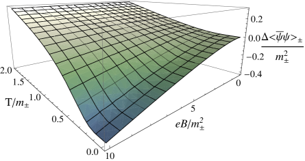
Figure 1: Temperature and magnetic field dependent fermion condensates as a function of $eB/m_{\pm}^{2}$ and $T/m_{\pm}$.

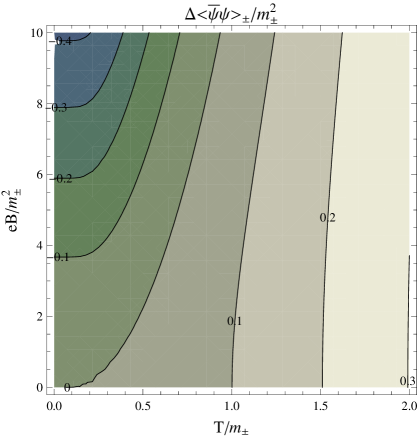
Figure 2: Contour plot for the temperature and magnetic field dependent fermion condensates as a function of $eB/m_{\pm}^{2}$ and $T/m_{\pm}$.

The exact expression for the condensates is plotted in Fig. 1. Due to the fact that the functional dependence of the condensates upon their respective bare masses is the same, we have defined dimensionless quantities in terms of the corresponding powers of $m_{\pm}$. The combined effects of the two agents on these quantities are such that at high temperatures and weak magnetic fields, the condensates are positive, but in the opposite regime when temperatures are low and the magnetic field is intense, it pulls down the condensates to their large negative values. In the region where the condensates do not deviate much from its zero value, temperature and magnetic field tend to nullify the effect of each other, as can be better seen from the contour plot displayed in Fig. 2. Of course the numerical details which define the intense and weak magnetic field limit for each fermion species depend on the value of the parameter $a=m_{o}/m$. As $\Delta\langle\bar{\psi}\psi\rangle_{\pm}=0$ would correspond to two different criticality curves, one deduces that there exist two critical temperatures. $T_{c}^{+}$ renders $\langle\bar{\psi}\psi\rangle_{+}=0$ while $\langle\bar{\psi}\psi\rangle_{-}\neq 0$ and $T_{c}^{-}$ guarantees $\langle\bar{\psi}\psi\rangle_{-}=0$, preserving $\langle\bar{\psi}\psi\rangle_{+}\neq 0$. This is better seen in Fig. 3, where the behavior of $T_{c}$ as a function of $eB$ for different values of a mass parameter $\tilde{m}$ is displayed. The critical temperature behaves as

$$T_{c}^{2}=\alpha({\tilde{m}}){\tilde{m}}^{2}+\kappa({\tilde{m}})\left(eB\right)^{1-\delta({\tilde{m}})}$$ (13)

$\tilde{m}$	$\alpha({\tilde{m}})$	$\kappa(\tilde{m})$	$\delta({\tilde{m}})$
1/20	0.0228	0.0583	0.0031
1/15	0.0235	0.0584	0.0031
1/10	0.0278	0.0586	0.0050
1/5	0.0410	0.0586	0.0110
1	0.0767	0.0627	0.0567
5	0.3088	0.0807	0.1397
10	0.8783	0.0977	0.1688
15	1.4696	0.1079	0.2256
20	2.1292	0.1144	0.2931

Table 1: Fit parameters for Eq. (13) in units of ${\tilde{m}}_{0}=0.05$.

The parameters are listed in Table 1 for different multiples of ${\tilde{m}_{0}}=0.05$. Note that as $\tilde{m}\to 0$, $\delta({\tilde{m}})\to 0$ and $\kappa({\tilde{m}})\to 0.0583$. For small values of mass, curves for the critical temperature are hardly distinguishable. A similar behavior was found in Ref. Farakos:1998 for the parity-preserving case. Moreover, the dependence of $T_{c}$ on mass becomes stronger as $\tilde{m}$ grows bigger. This implies that as $a\to 1$, $T_{c}^{+}$ depends more conspicuously on the mass, whereas $T_{c}^{-}$ is roughly independent of it.

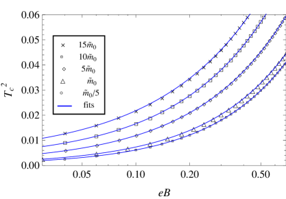
Figure 3: Critical temperature squared vs. magnetic field for different masses. Solid lines represent the fit in Eq. (13).

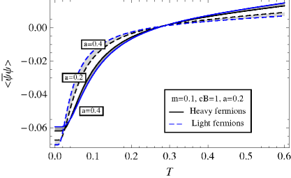
Figure 4: Temperature dependent condensates as a function of $T$ at fixed $eB=1$ and $m=0.1$ for $0.2\leq a\leq 0.4$. Light-shadowed region between dashed lines: Light-fermion condensate. Dark-shadowed region between solid lines: Heavy-fermion condensate.

Figure 4 displays the temperature dependent light- and heavy-fermion condensates for $0.1\leq a\leq 0.2$ at fixed $eB=1$ and $m=0.1$. We observe that for low temperatures, the effects of the magnetic field are dominant, as expected. The lighter the fermions, the more visible these effects are. As temperature increases, thermal effects start dominating the fermion condensation. In a selected range of values of $a$, we observe that the thermal effects for moderate values of $T$ are enhanced for light-fermions, but for heavy-fermions, thermal effects are more visible at sufficiently higher temperatures.

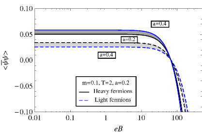
Figure 5: Magnetic field dependent condensates as a function of $eB$ at fixed $T=2$ and $m=0.1$ for $0.2\leq a\leq 0.4$. Light-shadowed region between dashed lines: Light-fermion condensate. Dark-shadowed region between solid lines: Heavy-fermion condensate.

In Fig. 5, we show the magnetic field dependence of the condensates for fixed values of $T$ ($T=2$) and $m$ ($m=0.1$). The parallel behavior of the two condensates seems to be affected only by the magnitude of the light- and heavy-fermion mass, and not necessarily by the parity-violating nature of $m_{o}$. Such an effect, however, might be evident at the non-perturbative level Edward . In this connection, study of the dynamical mass generation and the corresponding calculation of the thermal conductivity is currently under way Enif:2011 . Once the condensates have been evaluated, we can relate them with the Schwinger effect as we show in the next section.

IV Effective Lagrangian

An interesting application of our findings comes from the relation which exists between the condensate and the one-loop effective Lagrangian ${\cal L}^{(1)}$ schwinger ; gies

$$\langle\bar{\psi}\psi\rangle_{\pm}=-\frac{\partial{\cal L}^{(1)}_{\pm}}{\partial m_{\pm}}\;$$ (14)

in an external electromagnetic field. In this section we shall obtain the magnetization of a gas of noninteracting fermions andersen through this effective Lagrangian in the presence of a constant magnetic field. As a second application, by replacing $eB\rightarrow-ieE$, we derive this quantity in an external uniform electric field and compare against the Schwinger formula for pair production.

IV.1 Magnetization

Let us now proceed with the calculation of the magnetization of a gas of Dirac fermions of light and heavy species. The one-loop effective Lagrangian for each species at zero temperature in the presence of a magnetic field is simply given as

$${\cal L}^{(1)}_{\pm}=-\frac{1}{8\pi^{\frac{3}{2}}}\int_{0}^{\infty}\frac{ds\ e^{-sm^{2}_{\pm}}}{s^{\frac{5}{2}}}\left[eBs\coth{(eBs)}-1\right]\>.$$ (15)

Therefore, the magnetization $M_{\pm}={\partial{\cal L}_{\pm}^{(1)}}/{\partial B}$ for each species is

$$M_{\pm} = -\frac{e}{8\pi^{\frac{3}{2}}}\int_{0}^{\infty}\frac{ds\ e^{-sm^{2}_{\pm}}}{s^{\frac{3}{2}}}$$ (16)

$$\times\Bigg{[}\coth{(eBs)}-\frac{eBs}{\sinh^{2}{(eBs)}}\Bigg{]}\;.$$

In the weak field limit, expanding the expression in the square bracket and by direct integration, we find that

$$M_{\pm}=-\frac{e^{2}B}{12\pi m_{\pm}};$$ (17)

Expectedly, the magnetization grows linearly with the magnetic field and vanishes in its absence. Moreover, it is larger for the light species. The strong field case is better seen by writing Eq. (16) in the equivalent form

$$M_{\pm} = -\frac{em_{\pm}}{4\pi}-\frac{em^{2}_{\pm}}{\sqrt{32}\pi\sqrt{eB}}\zeta\left(\frac{1}{2},\frac{m^{2}_{\pm}}{2eB}\right)$$ (18)

$$+\frac{3e\sqrt{eB}}{\sqrt{8}\pi}\zeta\left(-\frac{1}{2},\frac{m^{2}_{\pm}}{2eB}\right)\;,$$

where $\zeta{(a,x)}$ is the Hurwitz-zeta function. Thus, taking the limit $m_{\pm}<<\sqrt{eB}$, we find that

$$M_{\pm}=\frac{3e\sqrt{eB}\zeta\left(-\frac{1}{2}\right)}{\sqrt{8}\pi}\;.$$ (19)

Here, $\zeta(x)$ is the Riemann-zeta function. Thus the linear dependence gets transformed into a square-root dependence for intense magnetic fields. After taking into account the fcator of 2 for the fermion species, expressions (18) and (19) compare correctly with the results which can be inferred from Eqs. (A4, 7.4) of Sharapov respectively.

Following the same reasoning, the effects of a thermal bath yield the following expression for the magnetization

$$M_{\pm} = -\frac{e}{8\pi^{\frac{3}{2}}}\int_{0}^{\infty}\frac{ds\ e^{-sm^{2}_{\pm}}}{s^{\frac{3}{2}}}\Theta_{4}\left(0,e^{-\frac{1}{4T^{2}s}}\right)$$ (20)

$$\times\Bigg{[}\coth{(eBs)}-\frac{eBs}{\sinh^{2}{(eBs)}}\Bigg{]}\;.$$

Again, assuming $eB$ to be the smallest energy scale, we have that

$$M_{\pm}=-\frac{e^{2}B}{12\pi m_{\pm}}\left(1-2\tilde{n}(m_{\pm})\right)\;,$$ (21)

which reduces to

$$M_{\pm}=-\frac{e^{2}B}{24\pi T}\;$$ (22)

at high temperatures. Thus in the high temperature limit, we recover the free case, as can be observed in Fig. 6. This is expected since in this regime, the effective Lagrangian approaches the thermodynamic potential for a gas of non interacting massive fermions. However, if $T\ll m_{\pm}$, the magnetization for each fermion species reduces to the vacuum case, Eq. (17), which agrees with the result of Ref. andersen for each species.

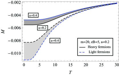
Figure 6: Magnetization as a function of $T$ at fixed $m=20$ and $B=5$ for $0.2\leq a\leq 0.4$. Light-shadowed region between dashed lines: Light-fermion. Dark-shadowed region between solid lines: Heavy-fermion.

In order to obtain the strong magnetic field behavior, let us focus on the thermal part of Eq. (11) alone. The vacuum part corresponds to Eq. (19). We integrate term by term with respect to $m_{\pm}$ the infinite sum and then differentiate with respect to $B$. Thus the thermal part of the magnetization can be expressed as

$$M_{\pm}^{T} = -\frac{e}{2\pi}\sum_{l=0}^{\infty}\left[\frac{eBl\ {\tilde{n}}(\sqrt{2eBl+m_{\pm}^{2}})}{\sqrt{2eBl+m_{\pm}^{2}}}\right.$$ (23)

$$\left.-T\ln(1+e^{-\sqrt{2eBl+m_{\pm}^{2}}/T})\right]\;,$$

In the strong field limit, we have

$$M_{\pm}^{T} = -\frac{e}{2\pi}\sum_{l=0}^{\infty}\left[\frac{\sqrt{eBl}\ {\tilde{n}}(\sqrt{2eBl})}{\sqrt{2}}\right.$$ (24)

$$\left.-T\ln\left(1+e^{-\sqrt{2eBl}/T}\right)\right]\;,$$

which is dominated by the $l=0$, magnetic field independent contribution. Higher Landau levels are exponentially suppressed. The contribution to the magnetization for the $l=0$ and $l=1$ levels, along with the vacuum contribution thus yields

$$M_{\pm} = -\frac{e\sqrt{eB}e^{-\frac{\sqrt{2eB}}{T}}}{\sqrt{8}\pi}+\frac{eT\ln(2)}{2\pi}$$ (25)

$$+\frac{3e\sqrt{eB}}{\sqrt{8}\pi}\zeta\left(-\frac{1}{2}\right)\;.$$

The last term, which corresponds to the vacuum contribution, leads the behavior of the magnetization in this regime. The weak- and strong magnetic field behavior of the magnetization are illustrated in Fig. 7. The strong field approximation, Eq. (25), which is a much simpler expression than Eq. (20), lies on top of the exact result for intense fields. When the fields are weak, the corresponding limit, Eq. (22) describes the exact result perfectly well. Note that it is not possible to appreciate the difference between the three results in that region due to the smallness of $M_{\pm}$ and the fact that the plot has been drawn on a logarithmic scale along the $x$-axis.

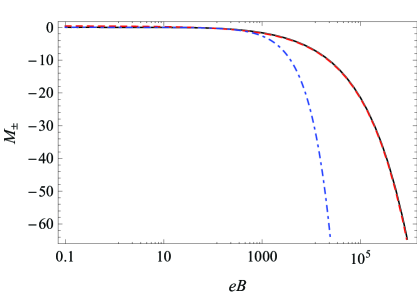
Figure 7: Magnetization as a function of $eB$ at fixed ${\tilde{m}}=0.05$ and $T=5$. Solid-line: Exact result, Eq. (20); Dashed-line: Strong field limit, Eq. (25); Dot–dashed-line: Weak field result, Eq. (22).

Next we consider the pair production rate.

IV.2 Pair production

We can perform a consistency check of our findings against the Schwinger’s formula for pair production, Ref. schwinger . Let us remember that the Schwinger mechanism is understood in terms of an imaginary part developed by the effective action due to the instability caused by an intense uniform electric field. Such an imaginary part is readily obtained from the condensate by simply replacing $eB\rightarrow-ieE$, i.e.,

$$\Delta\langle\bar{\psi}\psi\rangle^{E}_{\pm}=-\frac{m_{\pm}}{4\pi^{\frac{3}{2}}}\int_{0}^{\infty}\frac{d\eta}{\eta^{\frac{3}{2}}}e^{-\eta m_{\pm}^{2}}\left[eE\eta\cot(eE\eta)-1\right].$$ (26)

Using the identity

$$\cot(eE\eta)=\frac{1}{eE\eta}+\sum_{n=1}^{\infty}\sum_{s=\pm 1}\frac{1}{eE\eta+sn\pi}$$ (27)

in Eq. (26), we get

$$\Delta\langle\bar{\psi}\psi\rangle^{E}_{\pm}=-\frac{m_{\pm}eE}{4\pi^{\frac{3}{2}}}\sum_{n=1}^{\infty}\sum_{s=\pm 1}\int_{0}^{\infty}\frac{d\eta}{\eta^{\frac{1}{2}}}\frac{e^{-m_{\pm}^{2}\eta}}{eE\eta+sn\pi}\;.$$ (28)

In order to obtain the pair production probability, we use the prescription $m_{\pm}^{2}\rightarrow m_{\pm}^{2}+i\epsilon$ in Eq. (28). It is equivalent to moving the cotangent poles by an amount “$i\epsilon$” above the $Re(\eta)$ axis. Thus, it is easy to show that the imaginary part of the condensate in the presence of an electric field is

$$Im[\Delta\langle\bar{\psi}\psi\rangle_{\pm}^{E}] = -\frac{m_{\pm}eE}{4\pi^{\frac{1}{2}}}\sum_{n=1}^{\infty}\sum_{s=\pm 1}\int_{0}^{\infty}\frac{d\eta}{\eta^{\frac{1}{2}}}e^{-m_{\pm}^{2}\eta}$$ (29)

$$\hskip 28.45274pt\times\delta(eE\eta+sn\pi)$$

$$= -\frac{m_{\pm}(eE)^{\frac{1}{2}}}{4\pi}\sum_{n=1}^{\infty}\frac{e^{-\frac{m_{\pm}^{2}}{eE}n\pi}}{n^{\frac{1}{2}}}\;.$$

Therefore, the pair production rate is, Gusynin:1999 ,

$$2Im[{\cal L}^{(1)}_{\pm}]=\frac{1}{4\pi^{2}}(eE)^{\frac{3}{2}}\sum_{n=1}^{\infty}\frac{e^{-(\pi m_{\pm}^{2}/eE)n}}{n^{\frac{3}{2}}}\;.$$ (30)

Recall that the total rate is given by the first term in the summation alone. This result can be straightforwardly generalized to the case of parity violating mass terms considering now the light- and heavy-fermion species, shown in Fig. 8. Expectedly, increasing the intensity of the electric field, lighter fermions are much easier to produce than heavy ones. Thus, parity-violating effects favor the production of the light species over the heavy one.

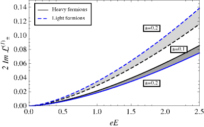
Figure 8: Pair production rate as a function of $eE$ at fixed $m=0.1$ for $0.1\leq a\leq 0.2$. Light-shadowed region between dashed lines: Light-fermion. Dark-shadowed region between solid lines: Heavy-fermion.

V Conclusions

We study the temperature and magnetic field dependence of the fermion anti-fermion condensate for planar QED, allowing for the parity violating mass terms. The 4-component study of this Lagrangian naturally leads us to consider two species of fermions which are non-degenerate in mass. Correspondingly, there are two types of condensates, with the magnetic field and temperature pulling them apart in diametrically opposed directions. The effects of the external ingredients are more pronounced for the lighter species of fermions as compared to the heavier one. We carry out a detailed quantitative analysis of this statement. Moreover, we also compute the magnetization induced by the magnetic fields and the pair production rate for both the species in the presence of an external electric field. For the former case, the magnetization becomes independent of the mass of each species as the field increases, but it vanishes when the temperature gets higher. In the later case, with the increasing electric field intensity, it is relatively easier to produce pairs of light species. For the mass $m=0.1$, the production rate for the light pairs is twice as much as that of the heavy species for the electric field intensity of the order of 3, as shown in the Fig. 8. Keeping in mind that the parity violating 2+1-dimensional Lagrangian has a host of applications in various condensed matter systems, we expect our results to have important bearing on their studies.

APPENDIX

Below we analyze different scenarios of relative strengths of the mass $m$ (for a general discussion in this appendix, we adopt the notation ${\tilde{m}}$ instead of $m_{\pm}$ and $\langle\bar{\psi}\psi\rangle$ instead of $\langle\bar{\psi}\psi\rangle_{\pm}$ ), the magnetic field $eB$ and the temperature $T$, namely, intense magnetic fields, i.e., ${\tilde{m}}\ll T\ll\sqrt{eB}$, intermediate magnetic fields, ${\tilde{m}}\ll\sqrt{eB}\ll T$, and weak magnetic fields, $\sqrt{eB}\ll{\tilde{m}}\ll T$. In these limits, we obtain uncomplicated and closed expressions. What is interesting is that in some cases, these simple results can be used instead of the complete Eq. (12) in all ranges of relative strengths of the energy scales involved without losing the quantitative precision by a significant margin. Some of these results can be compared and contrasted with the ones obtained in Anguiano:2007 ; Farakos:1998 .

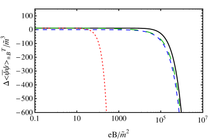
Figure 9: Temperature and field dependent fermion condensate in the units of ${\tilde{m}}^{2}$ as a function of $eB/{\tilde{m}}^{2}$ at fixed $T$. Solid line: exact result, Eq. (12). Dashed line: strong field limit, Eq. (31). Long-dashed line: intermediate field limit, Eq. (33). Dotted line: weak field limit, Eq. (37).

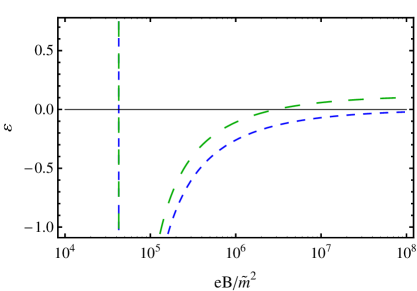
Figure 10: Relative error of the condensate. Dashed line: strong field asymptotics, Eq. (32). Long-Dashed line: intermediate field asymptotics, Eq. (34).

V.1 Strong field limit

Assuming the strength of the magnetic field to be the largest of the energy scales involved, the main contribution to the condensate comes from the lowest Landau level, $l=0$, which takes the form

$$\Delta\langle\bar{\psi}\psi\rangle_{B}^{T}=-\frac{eB}{4\pi}\left[1-2\tilde{n}({\tilde{m}})\right]\;.$$ (31)

Furthermore, when ${\tilde{m}}\ll T$, the leading contribution to the condensate is then given by

$$\Delta\langle\bar{\psi}\psi\rangle_{B}^{T}=-\frac{eB}{8\pi}\frac{{\tilde{m}}}{T}\;.$$ (32)

A comparison against the exact result is shown in Fig. 9. The dashed curve, that corresponds to the expression in Eq. (31), approaches the exact result (solid curve) as the strength of the field increases.

V.2 Intermediate Field

In order to obtain the intermediate field limit, we perform a high temperature expansion in the Fermi-Dirac distribution in Eq. (11). The leading term in this series can be written as follows

$$\Delta\langle\bar{\psi}\psi\rangle_{B}^{T} = \frac{{\tilde{m}}eB}{4\pi^{\frac{3}{2}}}\int_{\frac{3}{2\pi^{2}T^{2}}}^{\infty}\frac{d\eta}{\eta^{\frac{1}{2}}}e^{-\eta{\tilde{m}}^{2}}\coth(eB\eta)$$ (33)

$$-\frac{eB}{4\pi}\;,$$

where we have introduced an ultraviolet cutoff $(2/3)\pi^{2}T^{2}$ due to the fact that in the limit $eB\rightarrow 0$, each component of the transverse momentum contributes to the thermal bath with a factor $(1/3)\pi^{2}T^{2}$. Notice that in Fig. 5 the behavior of Eq. (33), displayed as the long-dashed curve, resembles the strong field behavior for large values of $eB$. In order to see the difference between Eqs. (31) and (33), we consider the regime where ${\tilde{m}}^{2}\ll eB$ in Eq. (33), which yields the following leading contribution to the condensate,

$$\Delta\langle\bar{\psi}\psi\rangle_{B}^{T} = -\sqrt{\frac{24}{\pi^{3}}}\frac{eB}{8\pi}\frac{{\tilde{m}}}{T}+\mathcal{O}\left(eB\frac{{\tilde{m}}^{3}}{T^{3}}\right)\;.$$ (34)

Comparing Eqs. (34) and (32), we see that

$$\frac{\{\Delta\langle\bar{\psi}\psi\rangle_{B}^{T}\}_{inter}}{\{\Delta\langle\bar{\psi}\psi\rangle_{B}^{T}\}_{strong}}=\sqrt{\frac{24}{\pi^{3}}}\approx 0.879794\;,$$ (35)

so that the asymptotic behavior of Eq. (33) for large values of $eB$ has an error of $12\%$ compared to strong field approximation (Eq. (32)) which is the exact behavior in that region. It may appear that for large magnetic field, the curve with intermediate magnetic field strength approximates the exact result better than the one with large field limit! This is not quite the case. This is depicted in Fig. 10, where we show the relative error,

$$\varepsilon=\frac{\{\Delta\langle\bar{\psi}\psi\rangle_{B}^{T}\}_{exact}-\{\Delta\langle\bar{\psi}\psi\rangle_{B}^{T}\}_{asymp}}{\{\Delta\langle\bar{\psi}\psi\rangle_{B}^{T}\}_{exact}}\;,$$ (36)

of the condensate as a function of the field strength for the asymptotic expressions of strong and intermediate field regions, Eqs. (32) and (34), respectively. The curve with the intermediate field strength in fact overshoots the exact result for large magnetic fields.

V.3 Weak field limit

In the weak field limit, we perform a Taylor’s series for $eB\ll{\tilde{m}}^{2}$ in Eq. (12) and we get

$$\Delta\langle\bar{\psi}\psi\rangle_{B}^{T} = \Delta\langle\bar{\psi}\psi\rangle^{T}$$ (37)

$$+ \frac{(eB)^{2}\tilde{n}({\tilde{m}})}{12\pi{\tilde{m}}^{2}}\left[1+\frac{{\tilde{m}}}{T}(1-\tilde{n}({\tilde{m}}))\right]$$

$$- \frac{1}{24\pi}\frac{(eB)^{2}}{{\tilde{m}}^{2}}\;.$$

This expression is shown as a dotted line in Fig. (5), which neatly matches onto the exact result for weak fields.

References

- (1) A. Bashir, A. Raya, S. Sanchez-Madrigal and C.D. Roberts, Few Body Sys. 46, 229 (2009); A. Bashir and A. Raya, Few Body Sys. 41, 185 (2007).
- (2) D.J. Gross, R.D. Pisarski and L.G. Jaffe, Rev. Mod. Phys. 53, 43 (1981).
- (3) T.W. Appelquist and R. Pisarski, Phys. Rev. D 23, 2305 (1981).
- (4) A. Ayala and A. Bashir, Phys. Rev. D 67, 076005 (2003).
- (5) S.G. Sharapov, V.P. Gusynin and H. Beck, Phys. Rev. B 69, 075104 (2004).
- (6) N. Dorey and N.E. Mavromatos, Nucl. Phys. B 386, 614 (1992); K. Farakos and N.E. Mavromatos, Mod. Phys. Lett. A 13, 1019 (1998); M. Sutherland et. al., Phys. Rev. Lett. 94, 147004 (2005).
- (7) M. Franz and Z. Tesanovic, Phys. Rev. Lett. 87, 257003 (2001); O. Vafek, A. Melikyan, M. Franz and Z. Tesanovic, Phys. Rev. B 63, 134509 (2001); Z. Tesanovic, O. Vafek and M. Franz, Phys. Lett. B 69, 180511 (2002); I.F. Herbut, Phys. Rev. B 66, 094504 (2002); M. Franz, Z. Tesanovic and O. Vafek, Phys. Rev. B 66, 054535 (2002).
- (8) A.A. Nersesyan and G.E. Vachanadze, J. Low Temp Phys. 77, 293 (1989): X. Yang and C. Nayak, Phys. Rev. B 65, 064523 (2002).
- (9) G.W. Semenoff, Phys. Rev. Lett. 53, 2449 (1984); J. González, F. Guinea and M.A.H. Vozmediano, Nucl. Phys. B 406, 771 (1993); J, González, F. Guinea and M.A.H. Vozmediano, Phys. Rev. 63, 134421 (2001).
- (10) V.P. Gusynin and S.G. Sharapov, Phys. Rev. Lett. 95, 146801 (2005); K.S. Novoselov et. al., Nature 438, 197 (2005); Y. Zhang et. al, Nature 438, 201 (2005).
- (11) A.S. Vshivtsev, B.V. Magnitskii, V.Ch. Zhukovskii, and K.G. Klimenko, Phys. Part. Nucl. 29, 523 (1998); V. Ch. Zhukovsky, K.G. Klimenko, and V.V. Khudyakov, Theor. Math. Phys. 124, 1132 (2000) [Teor. Mat. Fiz. 124, 323 (2000)].
- (12) K. Krishana et. al., Science 235 1196 (1997).
- (13) R.B. Laughlin, Phys. Rev. Lett. 80 5188 (1998).
- (14) F.D.M. Haldane, Phys. Rev. Lett. 61 2015 (1988).
- (15) K. Shimizu, Prog. Theor. Phys. 74, 610 (1985); Ma. de J. Anguiano and A. Bashir, Few Body Syst. 37, 71 (2005). A. Raya y E. Reyes, J. Phys. A 41, 355401 (2008).
- (16) K.-I. Kondo, Int. T. Mod. Phys. A 11, 777 (1996).
- (17) A. Ayala, A. Bashir, A. Raya, and A. Sánchez, J. Phys. G 37, 015001 (2010).
- (18) J. Schwinger, Phys. Rev. 82, 664 (1951).
- (19) A. Chodos, K. Everding, D. A. Owen. Phys. Rev. D 42, 2881 (1990).
- (20) J. I. Kapusta, Finite Temperature Field Theory, 1st. edition, Cambridge University Press (1989), ISBN 0-521-35155-3.
- (21) K. Farakos, G. Koutsoumbas and N.E. Mavromatos, Phys. Lett. B 431, 147 (1998).
- (22) A. Raya and E. Reyes, Phys. Rev. D 82, 016004 (2010).
- (23) A. Bashir, E. Gutiérrez, A. Raya and A. Sánchez, work in progress.
- (24) W. Dittrich and H. Gies, Probing the quantum vacuum. Perturbative effective action approach in quantum electrodynamics and its application. Springer Tracts in Modern Physics 166, (2000). ISSN 0081-3869.
- (25) J.O. Andersen and T Haughset, Phys. Rev. D51, 3073 (1995).
- (26) V.P. Gusynin and I.A. Shovkovy, J. Math. Phys. 40, 5406 (1999).
- (27) M. de J. Anguiano, A. Bashir and A. Raya Phys. Rev. D 76, 127702 (2007).