Modeling electronic structure and transport properties of graphene with resonant scattering centers

Abstract

We present a detailed numerical study of the electronic properties of single-layer graphene with resonant (“hydrogen”) impurities and vacancies within a framework of noninteracting tight-binding model on a honeycomb lattice. The algorithms are based on the numerical solution of the time-dependent Schrödinger equation and applied to calculate the density of states,  quasieigenstates, AC and DC conductivities of large samples containing millions of atoms. Our results give a consistent picture of evolution of electronic structure and transport properties of functionalized graphene in a broad range of concentration of impurities (from graphene to graphane), and show that the formation of impurity band is the main factor determining electrical and optical properties at intermediate impurity concentrations, together with a gap opening when approaching the graphane limit.

I Introduction

The experimental realization of a single layer of carbon atoms arranged in a honeycomb lattice (graphene) has prompted huge activity in both experimental and theoretical physics communities (for reviews, see Refs. r1, ; r2, ; r3, ; r4, ; r5, ; r6, ; r7, ; Cresti2008, ; Mucciolo2010, ; Peres2010, ). Graphene in real experiments always has different kinds of disorder or impurities, such as ripples, adatoms, admolecules, etc. One of the most important problems in graphene physics, especially, keeping in mind potential applications of graphene in electronics, is understanding the effect of these imperfections on the electronic structure and transport properties.

Being massless Dirac fermions with the wavelength much larger than the interatomic distance, charge carriers in graphene scatter rather weakly by generic short-range scattering centers, similar to weak light scattering from obstacles with sizes much smaller that the wavelength. The scattering theory for Dirac electrons in two dimensions is discussed in Refs. Shon1998, ; Katsnelson2007, ; Hentschel2007, ; Novikov2007, . Long-range scattering centers are of special importance for transport properties, such as charge impurities r6 ; Nomura2006 ; Ando2006 ; Hwang2007 , ripples created long-range elastic deformations r7 ; Katsnelson2008 , and resonant scattering centers Peres2006 ; Katsnelson2007 ; Katsnelson2008 ; Ostrovsky2006 ; Stauber2007 ; Titov2010 . In the latter case, the divergence of the scattering length provides a long-range scattering and a very slow, logarithmic, decay of the scattering phase near the Dirac (neutrality) point. Earlier the resonant scattering of Dirac fermions was studied in a context of $d$-wave high-temperature superconductivity Altland2002 . For the case of graphene, vacancies are prototype examples of the resonant scatterers Stauber2007 ; Chen2009 . Numerous adatoms and admolecules (including the important case of hydrogen atoms covalently bonded with carbon atoms) provide other examples Wehling2008 ; Wehling2009 ; Wehling2009b . Recently, some experimental Ni2010 and theoretical Wehling2010 evidence appeared that, probably, the resonant scattering due to carbon-carbon bonds between organic admolecules and graphene is the main restricting factor for electron mobility in graphene on a substrate. Resonant scattering also plays an important role in interatomic interactions and ordering of adatoms on graphene Shytov2009 . This all makes the theoretical study of graphene with resonant scattering centers an important problem.

In the present paper, we study this issue by direct numerical simulations of electrons on a honeycomb lattice in the framework of the tight-binding model. Numerical calculations based on exact diagonalization can only treat samples with relative small number of sites, for example, to study the quasilocalization of eigenstate close to the neutrality point around the vacancy Peres2006 ; Pereira2008 and the splitting of zero-energy Landau levels in the presence of random nearest neighbor hoping Pereira2009 . For large graphene sheet with millions of atoms, the numerical calculation of an important property, the density of states (DOS), is mainly performed by the recursion method Pereira2008 ; Pereira2008b ; Pereira2006 and time-evolution method DeRaedt2008 ; Wehling2010 . The time-evolution method is based on numerical solution of time-dependent Schrödinger equation with additional averaging over random superposition of basis states. In this paper, we extend the method of Ref. Hams2000, to compute the eigenvalue distribution of very large matrices to the calculation of transport coefficients. It allows us to carry out calculations for rather large systems, up to hundreds of millions of sites, with a computational effort that increases only linearly with the system size. Furthermore, another extension of the time-evolution method yields the quasieigenstate, a random superposition of degenerate energy eigenstates, as well as the AC and DC Wehling2010 conductivities.

The numerical calculation of the conductivity is based on the Kubo formula of noninteracting electrons. The details of these algorithm will be given in this paper. Our numerical results are consistent with the results on hydrogenated graphene Bang2010 and graphene with vacancies Wu2010 , which are based on the numerical calculation of the Kubo-Greenwood formula Roche1997 . Another widely used method of the numerical study of electronic transport in graphene is the recursive Green’s function method Cresti2007 ; Lewenkopf2007 ; Zhu2010 ; Hilke2009 ; ZhangYY2008 ; LongW2008 ; ZhangYY2009 ; ZhangYY2009b ; Lherbier2008 ; Mucciolo2009 , which is generally applied to relatively small samples followed by averaging of many different configurations. The recursive Green’s function method is a powerful tool to calculate the electronic transport in small system such as graphene ribbons, while the method that we employ in this paper is more suitable for large systems having millions of atoms and therefore does not involve averaging over different realizations.

The paper is organized as follows. Section II gives a description of the tight-binding Hamiltonian of single layer graphene including different types of disorders or impurities, in the absence and presence of a perpendicular magnetic field. In section III, we first discuss briefly the numerical method used to calculate the DOS, and show the accuracy of this algorithm by comparing the analytical and numerical results for clean graphene. Then, based on the calculation the DOS, we discuss the effects of vacancies or resonant impurities to the electronic structure of graphene, including the broadening of the Landau levels and the split of zero Landau levels. In section IV, we introduce the concept of a quasieigenstates, and use it to show the quasilocalization of the states around the vacancies or resonant impurities. Sections V and VI give discussions of the AC and DC conductivities, respectively. The details of numerical methods and various examples are discussed in detail in each section. Finally a brief general discussion is given in section VII.

II Tight-binding model

The tight-binding Hamiltonian of a single-layer graphene is given by

$$H=H_{0}+H_{1}+H_{v}+H_{imp},$$ (1)

where $H_{0}$ derives from the nearest neighbor interactions of the carbon atoms:

$$H_{0}=-\sum_{<i,j>}t_{ij}c_{i}^{+}c_{j},$$ (2)

$H_{1}$ represents the next-nearest neighbor interactions of the carbon atoms:

$$H_{1}=-\sum_{<<i,j>>}t_{ij}^{\prime}c_{i}^{+}c_{j},$$ (3)

$H_{v}$ denotes the on-site potential of the carbon atoms:

$$H_{v}=\sum_{i}v_{i}c_{i}^{+}c_{i},$$ (4)

and $H_{imp}$ describes the resonant impurities:

$$H_{imp}=\varepsilon_{d}\sum_{i}d_{i}^{+}d_{i}+V\sum_{i}\left(d_{i}^{+}c_{i}+H.c.\right).$$ (5)

For discussions of the last term see, e.g. Refs. Wehling2009b, ; Robinson2008, .

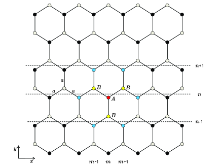
Figure 1: (Color online) The lattice structure of a graphene sheet. Each carbon is labeled by an coordinate $\left(m,n\right)$, where $m$ is along the zigzag edge and $n$ is along the armchair edge. Each carbon (red) has three nearest neighbors (yellow) and six next-nearest neighbors (blue).

The spin degree of freedom contributes only through a degeneracy factor and is omitted for simplicity in Eq. (1). Vacancies are introduced by simply removing the corresponding carbon atoms from the sample.

If a magnetic field is applied to the graphene layer, the hopping integrals are replaced by a Peierls substitution Vonsovsky1989 , that is, the hopping parameter becomes

$$t_{mn}\rightarrow t_{mn}e^{ie\int_{m}^{n}\mathbf{A}\cdot d\mathbf{l}}=t_{mn}e^{i\left(2\pi/\Phi_{0}\right)\int_{m}^{n}\mathbf{A}\cdot d\mathbf{l}},$$ (6)

where $\int_{m}^{n}\mathbf{A}\cdot d\mathbf{l}$ is the line integral of the vector potential from site $m$ to site $n$, and the flux quantum $\Phi_{0}=ch/e$.

Consider a single graphene layer with a perpendicular magnetic field $\mathbf{B}=(0,0,B)$. Let the zigzag edge be along the $x$ axis, and use the Landau gauge, that is, the vector potential $\mathbf{A}=(-By,0,0)$ Then $H_{0}$ changes into

$$H_{0} = \sum_{m,n}t_{\left(m,n\right),\left(m,n-1\right)}a_{m,n}^{+}b_{m,n-1}$$ (7)

$$+t_{\left(m,n\right),\left(m-1,n\right)}e^{i\pi n(\Phi/\Phi_{0})}a_{m,n}^{+}b_{m-1,n}$$

$$+t_{\left(m,n\right),\left(m+1,n\right)}e^{-i\pi n(\Phi/\Phi_{0})}a_{m,n}^{+}b_{m+1,n}$$

$$+H.c.$$

where

$$\Phi\equiv\frac{3\sqrt{3}}{2}Ba^{2},$$ (8)

$a$ is the nearest-neighbor interatomic distance.

III Density of States

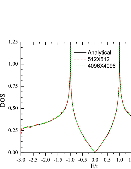
Figure 2: (Color online) Comparison of the analytical DOS (in units of $1/t$, black solid) with the numerical results of a sample contains $512\times 512$ (red dash) or $4096\times 4096$ (green dot) carbon atoms.

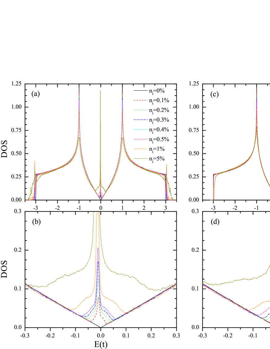
Figure 3: (Color online) Density of states (in units of $1/t$) as a function of energy $E$ (in units of $t$) for different resonant impurity ($\varepsilon_{d}=-t/16,$ $V=2t$) or vacancy concentrations: $n_{i}(n_{x})=0.1\%,$ $0.2\%,$ $0.3\%,$ $0.4\%,$ $0.5\%,$ $1\%,$ $5\%$. Sample size is $4096\times 4096.$

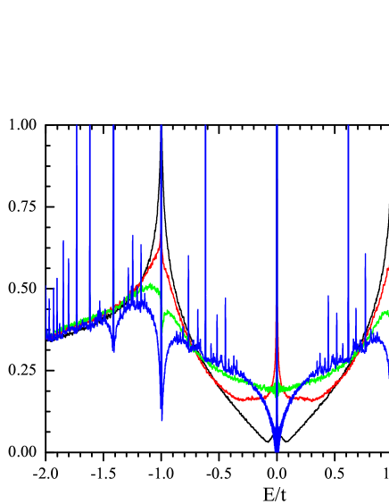
Figure 4: Density of states (in units of $1/t$) as a function of energy $E$ (in units of $t$) for the vacancies with large concentrations: $n_{x}=5\%,$ $10\%,$ $20\%,$ $30\%,$ $50\%,$ $90\%$. Sample size is $4096\times 4096$ for $n_{x}\leq 50\%$ and $8192\times 8192$ for $n_{x}=90\%$.

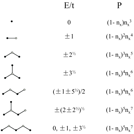
Figure 5: Typical atomic structures of most favourable isolated carbon groups in graphene with large concentration of vacancies. The energy eigenvalues of each group are listed in the central column (in units of $t$), and $P$ is the probability of a particular group to be found in a graphene sample.

Figure 6: Density of states (in units of $1/t$) as a function of energy $E$ (in units of $t$) for the resonant impurities ($\varepsilon_{d}=-t/16,$ $V=2t$) with large concentrations: $n_{i}=50\%,$ $90\%,$ $99\%,$ $99.5\%,$ $100\%$. Sample size is $2048\times 2048.$

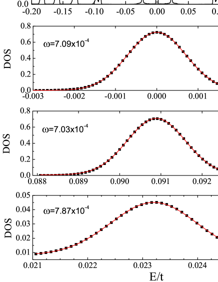
Figure 7: (Color online) Density of states (in units of $1/t$) as a function of energy $E$ (in units of $t$) in the presence of a uniform perpendicular magnetic field ($B=60T$) with vacancy concentration $n_{x}=0.01\%$. The red curves are Gaussian fits of Eq. (19) centered about each Landau levels, with $w=7.09\times 10^{-4}$ for $E_{N}=0$ $(N=0)$, $w=7.03\times 10^{-4}$ for $E_{N}=0.0909t$ $(N=1)$, and $w=7.87\times 10^{-4}$ for $E=0.0232t$ (between zero and first Landau levels). Sample size is $8192\times 8192.$

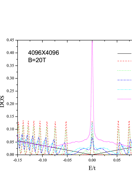
Figure 8: (Color online) Density of states (in units of $1/t$) as a function of energy $E$ (in units of $t$) in the presence of a uniform perpendicular magnetic field ($B=20T$) with different vacancy concentrations: $n_{x}=0\%,$ $0.01\%,$ $0.05\%,$ $0.1\%,$ $0.5\%$. Sample size is $4096\times 4096.$

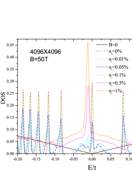
Figure 9: (Color online) Density of states (in units of $1/t$) as a function of energy $E$ (in units of $t$) in the presence of a uniform perpendicular magnetic field ($B=50T$) with different hydrogen concentrations $n_{i}=0\%,0.01\%,0.05\%,0.1\%,0.5\%,1\%$. Sample size is $4096\times 4096.$

The density of states describes the number of states at each energy level. An algorithm based on the evolution of time-dependent Schrödinger equation (TDSE) to find the eigenvalue distribution of very large matrices was described in Ref. Hams2000, . The main idea is to use a random superposition of all basis states as an initial state $\left|\varphi\left(0\right)\right\rangle$:

$$\left|\varphi\left(0\right)\right\rangle=\sum_{i}a_{i}\left|i\right\rangle,$$ (9)

where $\{\left|i\right\rangle\}$ are the basis states and $\{a_{i}\}$ are random complex numbers, solve the TDSE at equal time intervals, calculate the correlation function

$$\left\langle\varphi\left(0\right)\right|e^{-iHt}\left|\varphi\left(0\right)\right\rangle,$$ (10)

for each time step (we use units with $\hbar=1$): and then apply the Fourier transform to these correlation functions to get the local density of states (LDOS) on the initial state:

$$d\left(\varepsilon\right)=\frac{1}{2\pi}\int_{-\infty}^{\infty}e^{i\varepsilon t}\left\langle\varphi\left(0\right)\right|e^{-iHt}\left|\varphi\left(0\right)\right\rangle dt.$$ (11)

In practice the Fourier transform in Eq. (11) is performed by fast Fourier transformation (FFT). We use a Gaussian window to alleviate the effects of the finite time used in the numerical time integration of the TDSE. The number of time integration steps determines the energy resolution: Distinct eigenvalues that differ more than this resolution appear as separate peaks in the spectrum. If the eigenvalue is isolated from the rest of the spectrum, the width of the peak is determined by the number of time integration steps.

By averaging over different samples (random initial states) we obtain the density of states:

$$D\left(\varepsilon\right)=\lim_{S\rightarrow\infty}\frac{1}{S}\sum_{p=1}^{S}d_{p}\left(\varepsilon\right).$$ (12)

For a large enough system, for example, graphene crystallite consisting of $4096\times 4096\approx 1.6\times 10^{7}$ atoms, one initial random superposition state (RSS) is already sufficient to contain all the eigenstates, thus, its LDOS is approximately equal to the DOS of an infinite system, i.e.,

$$D\left(\varepsilon\right)\approx d\left(\varepsilon\right).$$ (13)

For the proof of this results and a detailed analysis of this method we refer to Ref. Hams2000, . To validate the method, we will compare the analytical and numerical results for clean graphene.

The numerical solution of the TDSE is carried out by using the Chebyshev polynomial algorithm, which is based on the polynomial representation of the operator $U\left(t\right)=e^{-itH}$ (see Appendix A). The Chebyshev polynomial algorithm is very efficient for the simulation of quantum systems and conserves the energy of the whole system to machine precision. In order to reduce the effects of the graphene edges on the electronic properties (see, e.g., Ref. DeRaedt2008, ), we use periodic boundary conditions for all the numerical results presented in this paper.

III.1 DOS of Clean Graphene

The analytical expression of the density of states of a clean graphene (ignoring the next-nearest neighbor interaction $t^{\prime}$ and the on-site energy) was given in Ref. Hobson1953, as

$$\rho\left(E\right)={\Huge\{}\begin{array}[]{c}\frac{2E}{t^{2}\pi^{2}}\frac{1}{\sqrt{F\left(E/t\right)}}\mathbf{K}\left(\frac{4E/t}{F\left(E/t\right)}\right),0<E<t,\\ \frac{2E}{t^{2}\pi^{2}}\frac{1}{\sqrt{4E/t}}\mathbf{K}\left(\frac{F\left(E/t\right)}{4E/t}\right),t<E<3t,\end{array}$$ (14)

where $F\left(x\right)$ is given by

$$F\left(x\right)=\left(1+x\right)^{2}-\frac{\left(x^{2}-1\right)^{2}}{4},$$ (15)

and $\mathbf{K}\left(m\right)$ is the elliptic integrals of first kind:

$$\mathbf{K}\left(m\right)=\int_{0}^{1}dx\left[\left(1-x^{2}\right)\left(1-mx^{2}\right)\right]^{-1/2}.$$ (16)

In Fig. 2, we compare the analytical expression Eq. (14) with the numerical results of the density of states for a clean graphene. One can clearly see that these numerical results fit very well the analytical expression, and the difference between the numerical and analytical results becomes smaller when using larger sample size (see the difference of a sample with $512\times 512$ or $4096\times 4096$ in Fig. 2). In fact, the local density of states of a sample containing $4096\times 4096$ is approximately the same as the density of states of infinite clean graphene, which indicates the high accuracy of the algorithm.

III.2 DOS of Graphene with Impurities

Next, we consider the influence of two types of defects on the DOS of graphene, namely, vacancies and resonant impurities. A vacancy can be regarded as an atom (lattice point) with and on-site energy $v\rightarrow\infty$ or with its hopping parameters to other sites being zero. In the numerical simulation, the simplest way to implement a vacancy it to remove the atom at the vacancy site. Introducing vacancies in a graphene sheet will create a zero energy modes (midgap state) Peres2006 ; Pereira2006 ; Pereira2008 . The exact analytical wave function associated with the zero mode induced by a single vacancy in a graphene sheet was obtained in Ref.Pereira2006, , showing a quasilocalized character with the amplitude of the wave function decaying as inverse distance to the vacancy. Graphene with a finite concentration of vacancies was studied numerically in Ref. Pereira2008, . The number of the midgap states increases with the concentration of the vacancies. The inclusion of vacancies brings an increase of spectral weight to the surrounding of the Dirac point ($E=0)$ and smears the van Hove singularities Peres2006 ; Pereira2008 . Our numerical results (see Fig. 3) confirm all these findings.

Resonant impurities are introduced by the formation of a chemical bond between a carbon atom from graphene sheet and a carbon/oxygen/hydrogen atom from an adsorbed organic molecule (CH₃, C₂H₅, CH₂OH, as well as H and OH groups)Wehling2010 . To be specific, we will call adsorbates hydrogen atoms but actually, the parameters for organic groups are almost the same Wehling2010 . The adsorbates are described by the Hamiltonian $H_{imp}$ in Eq. (1). The band parameters $V\approx 2t$ and $\epsilon_{d}\approx-t/16$ are obtained from the ab initio density functional theory (DFT) calculations Wehling2010 . As we can see from Fig. 3, small concentrations of vacancies or hydrogen impurities have similar effects to the DOS of graphene. Hydrogen adatoms also lead to zero modes and the quasilocalization of the low-energy eigenstates, as well as to smearing of the van Hove singularities. The shift of the central peak of the DOS with respect to the Dirac point in the case of hydrogen impurities is due to the nonzero (negative) on-site potentials $\epsilon_{d}$.

Now we consider the electronic structure of graphene with a higher concentration of defects. Large concentration of vacancies in graphene leads to well pronounced symmetric peaks in the DOS: a very high central peak at the Dirac point, two small peaks at the Van Hove singularities, and tiny peaks at $\left|E\right|/t=0.618,0.766,1.414,1.618,1.732,1.848$  (see Fig. 4). These results indicate the emergence of small pieces of isolated carbon groups, shown in Fig. 5. The positions of the peaks in the DOS match very well with the energy eigenvalues of these small subgroups. For example, non-interacting carbon atoms contribute to the peak at Dirac point, and isolated pairs contribute to the peaks at Van Hove singularities. Graphene with very high vacancy concentration, e.g., $n_{x}$ = 90%, is mainly a sheet of non-interacting carbon atoms, with small amount of isolated pairs, and tiny amounts of isolated triples. Only the peaks corresponding to these groups appear in the calculated DOS of $n_{x}$ = 90% in Fig. 4.

Graphene with $100\%$ concentration of hydrogen impurities is not graphene, but pure graphane Elias2009 . Graphane is shown to be an insulator because of the existence of a band gap (in our model, $2t$), see the bottom panel in Fig. 6. Graphene with large concentration ($n_{i}$) of hydrogen impurities corresponds to graphane with small concentrations ($1-n_{i}$) of vacancies of hydrogen atoms, which leads, again, to appearance of localized midgap states (shifted from zero due to nonzero $\epsilon_{d}$) on the carbon atoms which have no hopping integrals to any hydrogen, see these central peaks in Fig. 6. Despite the fact that our model is oversimplified for dealing with finite concentrations of hydrogen (in general, parameters of impurities should be concentration dependent, direct hopping between hydrogens should be taken into account, etc.), this conclusion is in an agreement with first principle calculations Lebegue2009 .

III.3 DOS of Graphene with Impurities in the Magnetic Field

A magnetic field perpendicular to a graphene layer leads to discrete Landau energy levels. The energy of the Landau levels of clean graphene is given by r2 ; r3

$$E_{N}=sgn(N)\sqrt{2e\hbar v_{F}^{2}B\left|N\right|},$$ (17)

where in the nearest-neighbor tight binding model

$$v_{F}/t=3a/2\hbar.$$ (18)

Our numerical calculations reproduces the positions of the Landau levels. Introducing impurities or disorders in graphene will broaden the Landau levels. Fig. 7 presents the numerical results for a uniform perpendicular magnetic field ($B=60T$) applied to a $8192\times 8192$ graphene sample with a small concentration of vacancies ($n_{x}=0.01\%$). The spectral distribution near each Landau level fits well to the Gaussian function

$$\rho\left(E\right)=A\exp\left[-\frac{\left(E-E_{N}\right)^{2}}{2w^{2}}\right],$$ (19)

with $w\approx 7\times 10^{-4}t$. Between two Laudau levels, there are extra peaks which also fit to a Gaussian distribution with $w\approx 8\times 10^{-4}t$. These additional localized states were also found in other numerical simulations Pereira2008b of much smaller $96\times 60$ samples with a stronger magnetic field ($B\approx 400T$) and larger concentration of vacancies ($n_{x}=0.21\%$ and $0.42\%$).

Increasing the concentration of the vacancies will smear and suppress the Landau levels except the one at zero energyPeres2006 , see Fig. 8. The zero-energy Landau level seems to be robust with respect to resonant impurities since the latter form their own midgap states.

The presence of hydrogen impurities has similar effects on the spectrum as in the case of vacancies (compare Fig. 8 and 9) except that, because of the non-zero on-site energy ($\epsilon_{d}$) of hydrogen sites, the zero-energy Landau level splits into two for a certain range of hydrogen concentrations (for example, see $n_{i}=0.05\%$ in Fig. 9). The peak at the neutrality point corresponds to the original zero-energy Landau level whereas the other one originates mainly from hybridization with hydrogen atoms. The splitting of zero-energy Landau level by other kinds of disorder is also observed, for example, with random nearest-neighbor hopping between carbon atoms as reported in Ref. Pereira2009, .

For small concentration of hydrogen impurities ($n_{i}=0.01\%$ in Fig. 9), there are also extra peaks between zero and first Landau levels, similar as in the case for low concentration of vacancies. The difference is that these two extra peaks are not symmetric around the neutrality point, because of non-zero on-site energy ($\epsilon_{d}$).

IV Quasieigenstates

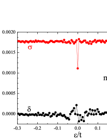
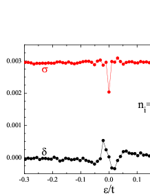
Figure 10: (Color online) The error ($\delta$ and $\sigma$) of the approximation of $\left|\Psi\left(\varepsilon\right)\right\rangle$ of a quasieigenstate in a graphene sample ($4096\times 4096$) with vacancies or hydrogen (($\varepsilon_{d}=-t/16,$ $V=2t$) impurities. The concentration of the defeats is $0.1\%$.

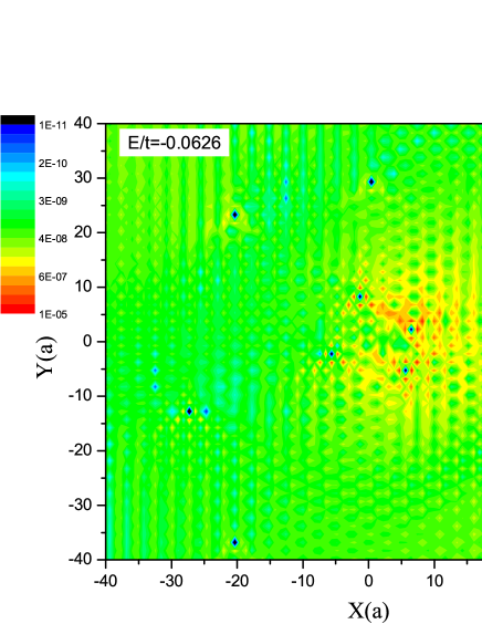
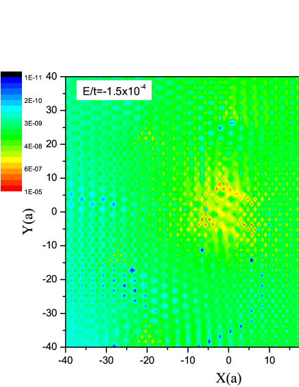
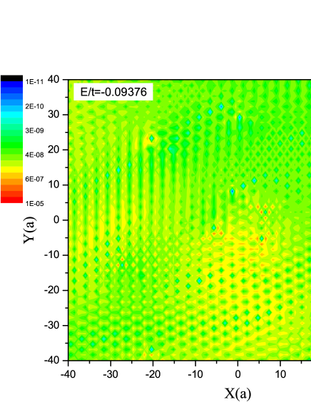
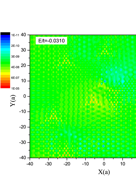
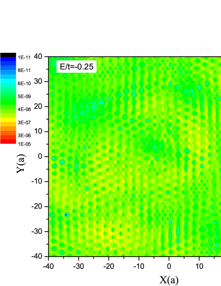
Figure 11: (Color online) Position of hydrogen impurities (black dots in the top left panel) and contour plot of the amplitudes of the quasieigenstates in the central part of a graphene sample ($4096\times 4096$) with different energies. The concentration of the hydrogen impurities ($\varepsilon_{d}=-t/16,$ $V=2t$) is $0.1\%$.

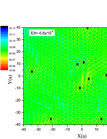
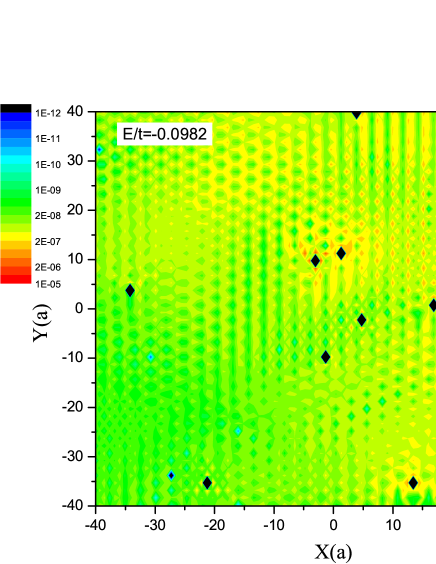
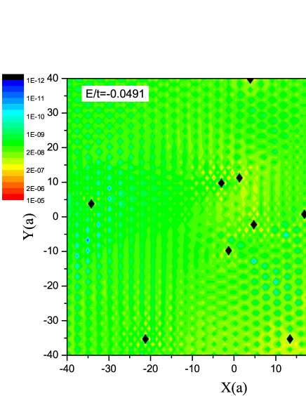
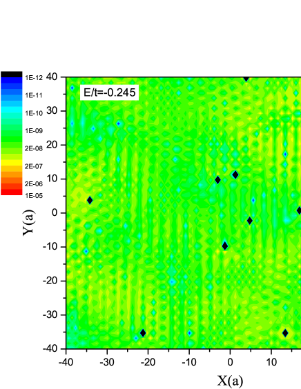
Figure 12: (Color online) Contour plot of the amplitudes of the quasieigenstates in the central part of a graphene sample ($4096\times 4096$) with different energies. The concentration of the vacancy impurities (indicated by black dots) is $0.1\%$.

For the general Hamiltonian (1) and for samples containing millions of carbon atoms, in practice, the eigenstates cannot be obtained directly from matrix diagonalization. An approximation of these eigenstates, or a superposition of degenerate eigenstates can be obtained by using the spectrum method Kosloffa1983 . Let $\left|\varphi\left(0\right)\right\rangle=\sum_{n}A_{n}\left|n\right\rangle$ be the initial state of the system, and $\{\left|n\right\rangle\}$ are the complete set of energy eigenstates. The state at time $t$ is

$$\left|\varphi\left(t\right)\right\rangle=e^{-iHt}\left|\varphi\left(0\right)\right\rangle.$$ (20)

Performing the Fourier transform of $\left|\varphi\left(t\right)\right\rangle$ one obtains the expression

$$\left|\widetilde{\Psi}\left(\varepsilon\right)\right\rangle = \frac{1}{2\pi}\int_{-\infty}^{\infty}dte^{i\varepsilon t}\left|\varphi\left(t\right)\right\rangle$$ (21)

$$= \frac{1}{2\pi}\sum_{n}A_{n}\int_{-\infty}^{\infty}dte^{i\left(\varepsilon-E_{n}\right)t}\left|n\right\rangle$$

$$= \sum_{n}A_{n}\delta\left(\varepsilon-E_{n}\right)\left|n\right\rangle,$$

which can be normalized as

$$\left|\Psi\left(\varepsilon\right)\right\rangle = \frac{1}{\sqrt{\sum_{n}\left|A_{n}\right|^{2}\delta\left(\varepsilon-E_{n}\right)}}\sum_{n}A_{n}\delta\left(\varepsilon-E_{n}\right)\left|n\right\rangle.$$

It is clear that $\left|\Psi\left(\varepsilon\right)\right\rangle$ is an eigenstate if it is a single (non-degenerate) state, and some superposition of degenerate eigenstates with the energy $\varepsilon$, otherwise.

In general, $\left|\Psi\left(\varepsilon\right)\right\rangle$ will not be an eigenstate but may be close to one and therefore we call it quasieigenstate. Although $\left|\Psi\left(\varepsilon\right)\right\rangle$ is written in the energy basis, the actual basis used to represent the state $\left|\varphi\left(t\right)\right\rangle$ can be any orthogonal and complete basis. It is convenient to introduce two variables $\delta\left(\varepsilon\right)$ and $\sigma\left(\varepsilon\right)$ to measure the difference between a true eigenstate and the quasieigenstate $\left|\Psi\left(\varepsilon\right)\right\rangle$:

$$\delta\left(\varepsilon\right) = \left\langle\Psi\left(\varepsilon\right)|H|\Psi\left(\varepsilon\right)\right\rangle-\varepsilon,$$ (23)

$$\sigma\left(\varepsilon\right) = \sqrt{\left\langle\Psi\left(\varepsilon\right)|H^{2}|\Psi\left(\varepsilon\right)\right\rangle-\left\langle\Psi\left(\varepsilon\right)|H|\Psi\left(\varepsilon\right)\right\rangle^{2}}.$$ (24)

As $\delta\left(\varepsilon\right)$ is a measure of the energy shift and $\sigma\left(\varepsilon\right)$ is the variance of the approximation, both variables should be zero if $\left|\Psi\left(\varepsilon\right)\right\rangle$ is a quasieigenstate with the energy $\varepsilon$. From numerical experiments (results not shown), we have found two ways to improve the accuracy of the quasieigenstates. One is that the Fourier transform should be performed on the states from both positive and negative times, and the other is that the wave function $\left|\varphi\left(t\right)\right\rangle$ should be multiplied by a window function (Hanning window NumericalRecipes ) $(1+\cos(\pi t/T))/2$ before performing the Fourier transform, $T$ being the final time of the propagation. The propagation in both positive and negative time is necessary to keep the original form of the integral in Eq. (21), and the use of a window improves the approximation to the integrals.

In Fig. 10 we show $\delta\left(\varepsilon\right)$ and $\sigma\left(\varepsilon\right)$ of the calculated quasieigenstates in graphene with vacancy or hydrogen impurities. The time step used in the propagation of the wave function is $\tau=1$ in the case of vacancies and $\tau=0.6$ in the case of hydrogen impurity. The total number of time steps is $N_{t}=$ $2048$ in both cases. One can see that the errors in the energy of $\left|\Psi\left(\varepsilon\right)\right\rangle$ are quite small ($\left|\delta\left(\varepsilon\right)\right|<5\times 10^{-4}$), and the standard deviation $\sigma\left(\varepsilon\right)$ is less than $2\times 10^{-3}$ and $3\times 10^{-3}$ for vacancies and hydrogen impurities, respectively. The value $\sigma\left(\varepsilon\right)$ is smaller in the case of the vacancies due to the larger time step and larger propagation time used. The fluctuations of $\delta\left(\varepsilon\right)$ in the region close to the neutrality point ($\varepsilon=0$) are due to the error introduced by the finite discrete Fourier transform in Eq. (21), because near the neutrality point, the finite discrete Fourier transform may mix components from the eigenstates in the opposite side of the spectrum. In fact, it would be more accurate to directly use $\left\langle\Psi\left(\varepsilon\right)|H|\Psi\left(\varepsilon\right)\right\rangle$ instead of $\varepsilon$ as the energy of the quasieigenstate. Notice that the error of $\sigma\left(\varepsilon\right)$ with $\varepsilon=0$ is smaller than in the case of nonzero $\varepsilon$, since for $\varepsilon=0$ there is no error due the combination of the factor $e^{i\varepsilon t}(=1)$ with the state $\left|\varphi\left(t\right)\right\rangle$. All the errors of $\delta\left(\varepsilon\right)$ and $\sigma\left(\varepsilon\right)$ as well as these fluctuations around $\delta\left(\varepsilon\right)$ can be reduced by increasing the time step $\tau$ and/or total number of time steps $N_{t}$.

Although quasieigenstates are not exact eigenstates, they can be used to calculate the electronic properties of the sample, such as the DC conductivity (as will be shown later). The contour plot of the amplitudes of the quasieigenstates directly reveals the structure of the eigenstates with certain eigenenergy, for example, the quasilocalization of the low-energy states around the vacancy or hydrogen impurity, see Fig. 11 and Fig. 12. The quasilocalization of the states around the impurities occurs not only for zero energy, but also for quasieigenstates with the energies close to the neutrality point. This quasilocalization leads to an increase of the spectral weight in the vicinity of the Dirac point ($E=0$), see Fig. 3. The states with larger eigenenergy are extended and robust to small concentration of impurities, and their spectral weight is close to that in clean graphene. One can see that in the case of hydrogen impurities, the quasieigenstates that are close enough to the impurity states, i.e., $E/t=-0.0626\approx\varepsilon_{d}$ in Fig. 11, are distributed in the whole region around hydrogen atoms. The carbon atoms coupled to hydrogens look like “vacancies”, with very small probability amplitudes, which explains why hydrogen impurities and vacancies produce similar effects on the electronic properties of graphene.

V Optical Conductivity

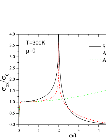
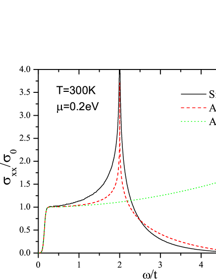
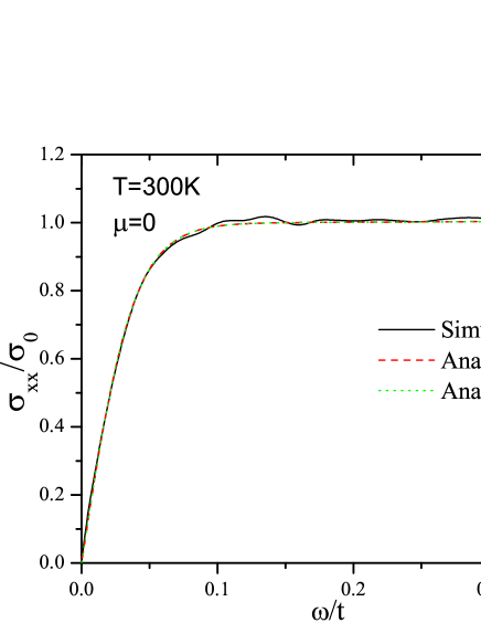
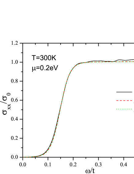
Figure 13: (Color online) Comparison of the numerically calculated optical conductivity ($\mu=0$ or $0.2$eV, $T=300K$) with Eq. (V.1) (analytical I) and Eq. (37) (analytical II). The size of the system is $M=N=8192$.

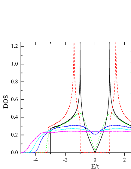
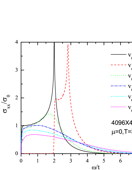
Figure 14: (Color online) Comparison of DOS (in units of $1/t$) and optical conductivity ($\mu=0,T=300K$) with symmetrical random ($v_{r}$) or antisymmetrical fixed ($\pm v_{d}$) potential on sublattices A and B. The size of the system is $M=N=4096$.

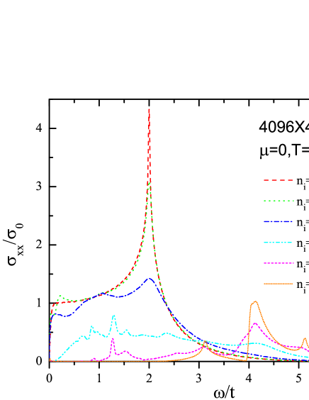
Figure 15: (Color online) Comparison of optical conductivity ($\mu=0,T=300K$) with different concentration of hydrogen impurities. The size of the system is $M=N=4096$, except for the clean graphene ($M=N=8192$).

Kubo’s formula for the optical conductivity can be expressed as Kubo1957

$$\mathbf{\sigma}_{\alpha\beta}\left(\omega\right) = \lim_{\varepsilon\rightarrow 0^{+}}\frac{1}{\left(\omega+i\varepsilon\right)\Omega}{\Huge\{}-i\left\langle\left[P_{\alpha},J_{\beta}\right]\right\rangle$$ (25)

$$+\int_{0}^{\infty}e^{i\left(\omega+i\varepsilon\right)t}dt\text{ }\left\langle\left[J_{\alpha}\left(t\right),J_{\beta}\right]\right\rangle{\Huge\}},$$

where $P$ is the polarization operator

$$P=e\sum_{i}\mathbf{r}_{i}c_{i}^{+}c_{i},$$ (26)

and $J$ is the current operator

$$J=\overset{\cdot}{P}=e\sum_{i}\overset{\cdot}{\mathbf{r}}_{i}c_{i}^{+}c_{i}=\frac{i}{\hbar}\left[H,P\right].$$ (27)

For a generic tight binding Hamiltonian, the current operator can be written as

$$J=-\frac{ie}{\hbar}\sum_{i,j}t_{ij}\left(\mathbf{r}_{j}-\mathbf{r}_{i}\right)c_{i}^{+}c_{j},$$ (28)

and

$$\left[P_{\alpha}\mathbf{,}J_{\beta}\right]=-\frac{ie^{2}}{\hbar}\sum_{i,j}t_{ij}\left[\left(\mathbf{r}_{i}-\mathbf{r}_{j}\right)_{\alpha}\left(\mathbf{r}_{j}-\mathbf{r}_{i}\right)_{\beta}\right]c_{i}^{+}c_{j}.$$ (29)

The ensemble average in Eq. (25) is over the Gibbs distribution, and the electric field is given by $\mathbf{E}\left(t\right)=\mathbf{E}_{0}\exp\left(i\omega+\varepsilon\right)t$ ($\varepsilon$ is a small parameter introduced in order that $\mathbf{E}\left(t\right)\rightarrow 0$ for $t\rightarrow-\infty$). In graphene, $P$ and $J$ are two-dimensional vectors, and $\Omega$ is replaced by the area of the sample $S$.

In general, the real part of the optical conductivity contains two parts, the Drude weight $D$ ($\omega=0$) and the regular part ($\omega\neq 0$). We omit the calculation of the Drude weight, and focus on the regular part. For non-interacting electrons, the regular part is Isihara1971

$$\text{Re}\sigma_{\alpha\beta}\left(\omega\right) = \lim_{\varepsilon\rightarrow 0^{+}}\frac{e^{-\beta\hbar\omega}-1}{\hbar\omega\Omega}\int_{0}^{\infty}e^{-\varepsilon t}\sin\omega t$$

$$\times 2\text{Im}\left\langle f\left(H\right)J_{\alpha}\left(t\right)\left[1-f\left(H\right)\right]J_{\beta}\right\rangle dt,$$

where $\beta=1/k_{B}T,$ $\mu$ is the chemical potential, and the Fermi-Dirac distribution operator

$$f\left(H\right)=\frac{1}{e^{\beta\left(H-\mu\right)}+1}.$$ (31)

In the numerical calculations, the average in Eq. (V) is performed over a random phase superposition of all the basis states in the real space, i.e., the same initial state $\left|\varphi\left(0\right)\right\rangle$ in calculation of DOS. The Fermi distribution operator $f\left(H\right)$ and $1-f\left(H\right)$ can be obtained by the standard Chebyshev polynomial decomposition (see Appendix B).

By introducing the three wave functions Iitaka1997

$$\left|\varphi_{1}\left(t\right)\right\rangle_{x} = e^{-\frac{iHt}{\hbar}}\left[1-f\left(H\right)\right]J_{x}\left|\varphi\right\rangle,$$ (32)

$$\left|\varphi_{1}\left(t\right)\right\rangle_{y} = e^{-\frac{iHt}{\hbar}}\left[1-f\left(H\right)\right]J_{y}\left|\varphi\right\rangle,$$ (33)

$$\left|\varphi_{2}\left(t\right)\right\rangle = e^{-\frac{iHt}{\hbar}}f\left(H\right)\left|\varphi\right\rangle,$$ (34)

we get all elements of the regular part of Re$\sigma_{\alpha\beta}\left(\omega\right)$:

$$\text{Re}\sigma_{\alpha\beta}\left(\omega\right) = \lim_{\varepsilon\rightarrow 0^{+}}\frac{e^{-\beta\hbar\omega}-1}{\hbar\omega\Omega}\int_{0}^{\infty}e^{-\varepsilon t}\sin\omega t$$ (35)

$$\times\left[2\text{Im}\text{ }\left\langle\varphi_{2}\left(t\right)\left|J_{\alpha}\right|\varphi_{1}\left(t\right)\right\rangle_{\beta}\right]dt.$$

V.1 Optical Conductivity of Clean Graphene

In Fig. 13, we compare our numerical results to the analytical results obtained in Refs. Stauber2008, ; Falkovsky2007, ; Kuzmenko2008, , where the real part of the conductivity in the visible region has the form Stauber2008

$$\text{Re}\sigma_{xx} = \sigma_{0}\left[\frac{\pi t^{2}a^{2}}{8A_{c}\hbar\omega}\rho\left(\frac{\hbar\omega}{2}\right)\left(18-\frac{\hbar^{2}\omega^{2}}{t^{2}}\right)+\frac{\hbar^{2}\omega^{2}}{4!2^{4}t^{2}}\right]$$

$$\left(\tanh\frac{\hbar\omega+2\mu}{4k_{B}T}+\tanh\frac{\hbar\omega-2\mu}{4k_{B}T}\right),$$

with the minimum conductivity $\sigma_{0}=\pi e^{2}/2h$. Around $\omega=0$ the real part of the conductivity can be simplified as Stauber2008 ; Falkovsky2007 ; Kuzmenko2008

$$\text{Re}\sigma_{xx} = \sigma_{0}\left(\frac{1}{2}+\frac{1}{72}\frac{\hbar^{2}\omega^{2}}{t^{2}}\right)$$ (37)

$$\left(\tanh\frac{\hbar\omega+2\mu}{4k_{B}T}+\tanh\frac{\hbar\omega-2\mu}{4k_{B}T}\right).$$

As we can see from Fig. 13, the numerical and analytical results match very well in the low frequency region, but not in the high frequence region. This is because the analytical expressions are partially based on the Dirac-cone approximation, i.e., the graphene energy bands are linearly dependent on the amplitude of the wave vector. It is exact for the calculations of the low-frequence optical conductivity, but not for high-frequence. Our numerical method does not use such approximation and has the same accuracy in the whole spectrum. Furthermore, our numerical results also show that the conductivity of Re$\sigma_{xx}$ with $\mu=0$ in the limit of $\omega=0$ converges to the minimum conductivity $\sigma_{0}$ when the temperature $T\rightarrow 0$.

V.2 Optical Conductivity of Graphene with Random on-Site Potentials

The on-site potential disorder can change the electronic properties of graphene dramatically. For example, if the potentials on sublattices A and B are not symmetric, a band gap will appear. If we set $v_{d}$ and $-v_{d}$ as the on-site potential on sublattice A and B, respectively, then a band gap of size $2v_{d}$ is observed in the central part of DOS and the optical conductivity in the region $0<\omega<2v_{d}$ becomes zero, see the red dashed lines ($v_{d}=t$) in Fig. (14). If the potentials on sublattice A and B are both uniformly random in a range $[-v_{r},v_{r}]$, then the spectrum is broaden symmetrically around the neutrality point (because of the random character of the potentials on sublattice A and B), and there is no band gap, see the colored lines (except the red one) in Fig. (14). It softens the singularities in the DOS, the smearing being larger for a larger degree of disorder. The smearing of the DOS leads to the smearing of the optical conductivity, see $\sigma_{xx}$ in Fig. 14.

V.3 Optical Conductivity of Graphene with Resonant Impurities

In Fig. 15 we present the optical conductivity of graphene with various concentrations of hydrogen impurities. Small concentrations of the impurities have a small effect on the optical conductivity, but higher concentrations change the optical properties dramatically, especially when the concentration reaches the maximum ($100\%$), i.e., when graphene becomes graphane. Graphane has a band gap ($2t$), see bottom panel in Fig. 6, which leads to the zero optical conductivities within the region $\left|\omega\right|\in[0,2t]$, see Fig. 15) for $n_{i}=100\%$. At intermediate concentrations, one can clearly see additional features in the optical conductivity related with the formation of impurity band. The Van Hove singularity of clean graphene is smeared out completely for concentrations as small as 1%.

VI DC Conductivity

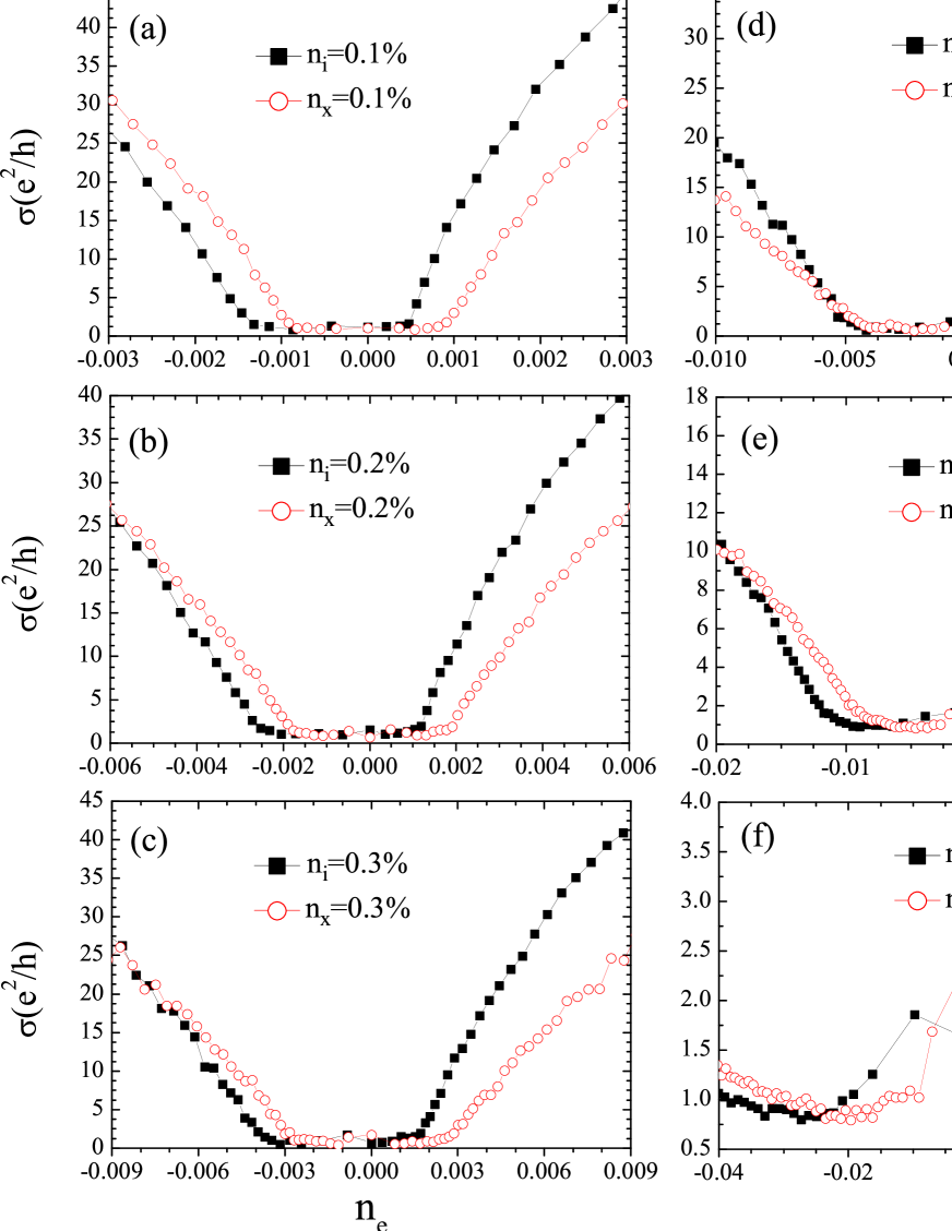
Figure 16: (Color online) Conductivity $\sigma$ (in units of $e^{2}/h$) as a function of charge carrier concentration $n_{e}$ (in units of electrons per atom) for different resonant impurity ($\varepsilon_{d}=-t/16,$ $V=2t$) or vacancy concentrations ($n_{x}$) : (a) $n_{i}=n_{x}=0.1\%,$ (b) $0.2\%,$ (c) $0.3\%,$ (d) $0.5\%$, (e) $1\%,$ (f) $5\%$. Numerical calculations are performed on samples containing (a) $8192\times 8192$ and (b-f) $4096\times 4096$ carbon atoms. The charge carrier concentrations $n_{e}$ are obtained by the integral of the corresponding density of states represented in Fig. 3.

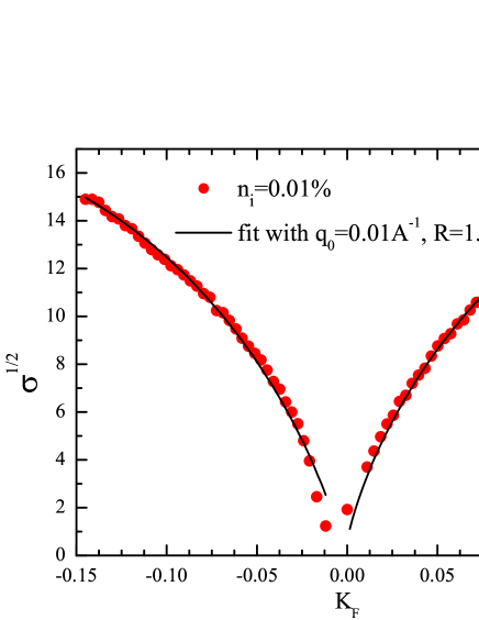
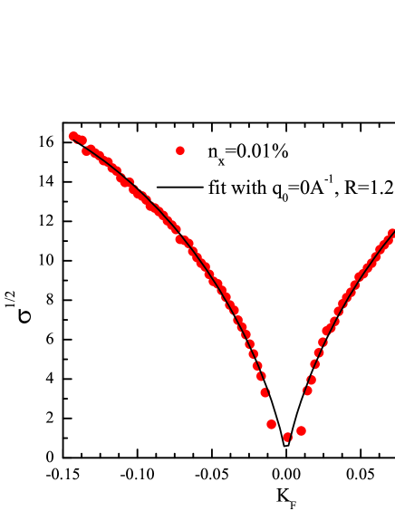
Figure 17: (Color online) Red dots: conductivity $\sigma$ (in units of $e^{2}/h$) as a function of $K_{F}$ (in units of Å^-1) for resonant impurity (top panel, $\varepsilon_{d}=-t/16,$ $V=2t$) or vacancy (bottom panel). The concentration of the impurities is $n_{i}=n_{x}=0.01\%.$ Numerical calculations are performed on samples containing $4096\times 4096$ carbon atoms. Black lines: fit of Eq. (44) with $q_{0}=0.01\text{\AA}^{-1}$, $R=1.25\text{\AA}$ for $n_{i}=0.01\%$, and $q_{0}=0$, $R=1.28\text{\AA}$ for $n_{x}=0.01\%$.

The DC conductivity can be obtained by taking $\omega\rightarrow 0$ in Eq. (25) yielding Isihara1971

$$\mathbf{\sigma}=-\frac{1}{V}Tr\left\{\frac{\partial f}{\partial H}\int_{0}^{\infty}dt\frac{1}{2}\left[JJ\left(t\right)+J\left(t\right)J\right]\right\}.$$ (38)

We can use the same algorithm as we used for the optical conductivity to perform the integration in Eq. (38), but it is not the best practical way since it only leads to the DC conductivity with one chemical potential each time, and the number of non-zero terms in Chebyshev polynomial representation growth exponentially when the temperature tends to zero. In fact, at zero temperature $\frac{\partial f}{\partial H}$ can be simplified as

$$-\frac{\partial f}{\partial H}=\delta\left(E_{F}-H\right),$$ (39)

and therefore Eq. (25) can be simplified as

$$\mathbf{\sigma}_{T=0} = \frac{\pi}{NV}\text{Re}\sum_{m,n=1}^{N}\left\langle n\right|J\left|m\right\rangle\left\langle m\right|J\left|n\right\rangle$$ (40)

$$\times\delta\left(E_{F}-E_{m}\right)\delta\left(E_{F}-E_{n}\right).$$

By using the quasieigenstates $\left|\Psi\left(\varepsilon\right)\right\rangle$ obtained from the spectrum method in Eq. (21), we can prove that (see Appendix C)

$$\mathbf{\sigma} = \frac{\rho\left(\varepsilon\right)}{V}\int_{0}^{\infty}dt\text{Re}\left[e^{-i\varepsilon t}\left\langle\varphi\right|Je^{iHt}J\left|\varepsilon\right\rangle\right]\approx\mathbf{\sigma}_{T=0},$$

where $\left|\varphi\right\rangle$ is the same initial random superposition state as in Eq. (20) and

$$\left|\varepsilon\right\rangle=\frac{1}{\left|\left\langle\varphi|\Psi\left(\varepsilon\right)\right\rangle\right|}\left|\Psi\left(\varepsilon\right)\right\rangle.$$ (42)

The accuracy of the quasieigenstates in Eq. (21) are mainly determined by the time interval and total time steps used in the Fourier transform. The main limitation of the numerical calculations using Eq. (21) is the size of the physical memory that can be used to store the quasieigenstates $\left|\Psi\left(\varepsilon\right)\right\rangle$.

We used the algorithm presented above to calculate the DC conductivity of single layer graphene with vacancies or resonant impurities. The results are shown in Fig. 16. As we can see from the numerical results, there is plateau of the order of the minimum conductivity Katsnelson2006 $4e^{2}/\pi h$ in the vicinity of the neutrality point, in agreement with theoretical expectations Ostrovsky2010 . Finite concentrations of resonant impurities lead to the formation of a low energy impurity band (see increased DOS at low energies in Fig. 3). At impurity concentrations of the order of a few percent (Fig. 16 e, f) this impurity band contributes to the conductivity and can lead to a maximum of $\sigma$ in the midgap region. The impurity band can host two electrons per impurity. For impurity concentrations below $\sim 5\%$, this leads to a plateau-shaped minimum of width $2n_{i}$ (or $2n_{x}$) in the conductivity vs. $n_{e}$ curves around the neutrality point. Analyzing experimental data of the plateau width (similar to the analysis for N₂O₄ acceptor states in Ref. Wehling2008, ) can therefore yield an independent estimate of impurity concentration.

Beyond the plateau around the neutrality point, the conductivity is inversely proportional to the concentration of the impurities, and approximately proportional to the carrier concentration $n_{e}$. This is consistent with the approach based on the Boltzmann equation, which in the limit of resonant impurities with $V\rightarrow\infty$, yields for the conductivity Katsnelson2007 ; Katsnelson2008 ; Robinson2008 ; Wehling2010

$$\sigma\approx(2e^{2}/h)\frac{2}{\pi}\frac{n_{e}}{n_{i}}\ln^{2}\left|\frac{E}{D}\right|,$$ (43)

where $n_{e}=E_{F}^{2}/D^{2}$ is the number of charge carriers per carbon atom, and $D$ is of order of the bandwidth. Equantion (43) yields the same behavior as for vacancies Stauber2007 . Note that for the case of the resonance shifted with respect to the neutrality point the consideration of Ref. Katsnelson2007, leads to the dependence

$$\sigma\propto\left(q_{0}\pm k_{F}\ln{k_{F}R}\right)^{2},$$ (44)

where $\pm$ corresponds to electron and hole doping, respectively, and $R$ is the effective impurity radius. The Boltzmann approach does not work near the neutrality point where quantum corrections are dominant Ostrovsky2006 ; Katsnelson2006 ; Auslender2007 . In the range of concentrations, where the Boltzmann approach is applicable the conductivity as a function of energy fits very well to the dependence given by Eq. (44), as for example shown in Fig. (17), with $q_{0}=0.01\text{\AA}^{-1}$, $R=1.25\text{\AA}$ for $n_{i}=0.01\%$, and $q_{0}=0$, $R=1.28\text{\AA}$ for $n_{x}=0.01\%$. The relation of these results to experiment is discussed in Ref. Wehling2010, .

The advantage of the method used here for the calculation of the DC conductivity is that the results do not depend on the upper time limit in the integration since the contributions to the integrand in Eq.(VI) corresponding to different energies tends to zero fast enough when the time is large. The propagation time for the integration depends on the concentration of the disorder, i.e., larger concentration leads to faster decay of the corrections. The disadvantage of this method is that a lot of memory may be needed to store the coefficients of many quasieigenstates. Furthermore, since $\left|\varepsilon\right\rangle$ in Eq. (42) contains the factor $1/\left|\left\langle\varphi|\Psi\left(\varepsilon\right)\right\rangle\right|$, this may cause problems when $\left|\left\langle\varphi|\Psi\left(\varepsilon\right)\right\rangle\right|$ is very small. For example, when using this method to calculate the Hall conductivity in the presence of strong magnetic fields, tiny $\left|\left\langle\varphi|\Psi\left(\varepsilon\right)\right\rangle\right|$ (out the Landau levels) will leads to large fluctuations of the calculated conductivity. Nevertheless, the conductivities without the presence on the magnetic filed in our paper are agreement with the results reported in Refs. Bang2010, (hydrogenated graphene) and Wu2010, (graphene with vacancies), and both papers are based on the numerical calculation of the Kubo-Greenwood formula, as proposed in Ref.Roche1997, . To calculate the Hall conductivity accurately our method should be developed further.

VII Summary

We have presented a detailed numerical study of the electronic properties of single-layer graphene with resonant (“hydrogen”) impurities and vacancies within a framework of noninteracting tight-binding model on the honeycomb lattice. The algorithms developed in this paper are based on the numerical solution of the time-dependent Schrödinger equation, the fundamental operation being the action of the evolution operator on a general wave vector. We do not need to diagonalize the Hamiltonian matrix to obtain the eigenstates and therefore the method can be applied to very large crystallites which contains millions of atoms. Furthermore since the operation of the Hamiltonian matrix on a general wave vector does not require any special symmetry of the matrix elements, this flexibility can be exploited to study different kinds of disorder and impurities in the noninteracting tight-binding model.

The algorithms for the calculation of density of states, quasieigenstates, AC and DC conductivities, are applicable to any 1D, 2D and 3D lattice structure, not only to a single layer of carbon atoms arranged in a honeycomb lattice. The calculation for the electronic properties of multilayer graphene can be easily obtained by adding the hoping between the corresponding atoms of different layers.

Our computational results give a consistent picture of behavior of the electronic structure and transport properties of functionalized graphene in a broad range of concentration of impurities (from graphene to graphane). Formation of impurity bands is the main factor determining electrical and optical properties at intermediate impurity concentrations, together with the appearance of a gap near the graphane limit.

VIII Acknowledgement

The support by the Stichting Fundamenteel Onderzoek der Materie (FOM) and the Netherlands National Computing Facilities foundation (NCF) are acknowledged.

IX Appendix A

Suppose $x\in\left[-1,1\right]$, then

$$e^{-izx}=J_{0}(z)+2\sum_{m=1}^{\infty}\left(-i\right)^{m}J_{m}\left(z\right)T_{m}\left(x\right),$$ (45)

where $J_{m}(z)$ is the Bessel function of integer order $m$, and $T_{m}\left(x\right)=\cos\left[m\arccos\left(x\right)\right]$ is the Chebyshev polynomial of the first kind. $T_{m}\left(x\right)$ obeys the following recurrence relation:

$$T_{m+1}\left(x\right)+T_{m-1}\left(x\right)=2xT_{m}\left(x\right).$$ (46)

Since the Hamiltonian $H$ has a complete set of eigenvectors $\left|E_{n}\right\rangle$ with real valued eigenvalues $E_{n}$, we can expand the wave function $\left|\phi(0)\right\rangle$ as a superposition of the eigenstates $\left|n\right\rangle$ of $H$

$$\left|\phi(0)\right\rangle=\sum_{n=1}^{N}\left|n\right\rangle\left\langle n|\phi(0)\right\rangle,$$ (47)

and therefore

$$\left|\phi(t)\right\rangle=e^{-itH}\left|\phi(0)\right\rangle=\sum_{n=1}^{N}e^{-itE_{n}}\left|n\right\rangle\left\langle n|\phi(0)\right\rangle.$$ (48)

By using the inequality

$$\left\|\sum X_{n}\right\|\leq\sum\left\|X_{n}\right\|,$$ (49)

with the Hamiltonian $H$ of Eq.(1) we find

$$\left\|H\right\|_{b} \equiv 3t_{\max}+6t_{\max}^{\prime}+\left|v\right|_{\max}+\left|\varepsilon_{d}\right|+\left|V\right|$$ (50)

$$\geqslant \max\{E_{n}\}.$$

Introduce new variables $\hat{t}\equiv t\left\|H\right\|_{b}$ and $\hat{E}_{n}\equiv E_{n}/\left\|H\right\|_{b}$, where $\hat{E}_{n}$ are the eigenvalues of a modified Hamiltonian $\hat{H}\equiv H/\left\|H\right\|_{b}$, that is

$$\hat{H}\left|E_{n}\right\rangle=\hat{E}_{n}\left|E_{n}\right\rangle.$$ (51)

By using Eq. (45), the time evolution of $\left|\phi(t)\right\rangle$ can be represented as

$$\left|\phi(t)\right\rangle = \left[J_{0}(\hat{t})\hat{T}_{0}\left(\hat{H}\right)+2\sum_{m=1}^{\infty}J_{m}\left(\hat{t}\right)\hat{T}_{m}\left(\hat{H}\right)\right]\left|\phi(0)\right\rangle,$$

where the modified Chebyshev polynomial $\hat{T}_{m}\left(\hat{E}_{n}\right)$ is

$$\hat{T}_{m}\left(\hat{E}_{n}\right)=\left(-i\right)^{m}T_{m}\left(\hat{E}_{n}\right),$$ (53)

obeys the recurrence relation

$$\hat{T}_{m+1}\left(\hat{H}\right)\left|\phi\right\rangle = -2i\hat{H}\hat{T}_{m}\left(\hat{H}\right)\left|\phi\right\rangle+\hat{T}_{m-1}\left(\hat{H}\right)\left|\phi\right\rangle,$$

$$\hat{T}_{0}\left(\hat{H}\right)\left|\phi\right\rangle = I\left|\phi\right\rangle,\hat{T}_{1}\left(\hat{H}\right)\left|\phi\right\rangle=-i\hat{H}\left|\phi\right\rangle.$$ (54)

X Appendix B

In general, a function $f(x)$ whose values are in the range $\left[-1,1\right]$ can be expressed as

$$f(x)=\frac{1}{2}c_{0}T_{0}\left(x\right)+\sum_{k=1}^{\infty}c_{k}T_{k}\left(x\right),$$ (55)

where $T_{k}\left(x\right)=\cos\left(k\arccos x\right)$ and the coefficients $c_{k}$ are

$$c_{k}=\frac{2}{\pi}\int_{-1}^{1}\frac{dx}{\sqrt{1-x^{2}}}f\left(x\right)T_{k}\left(x\right).$$ (56)

Let $x=\cos\theta$, then $T_{k}\left(x\right)=T_{k}\left(\cos\theta\right)=\cos k\theta$, and

$$c_{k} = \frac{2}{\pi}\int_{0}^{\pi}f\left(\cos\theta\right)\cos k\theta d\theta$$ (57)

$$= \text{Re}\left[\frac{2}{N}\sum_{n=0}^{N-1}f\left(\cos\frac{2\pi n}{N}\right)e^{\frac{2\pi ink}{N}}\right],$$

which can be calculated by the fast Fourier transform.

For the operators $f=ze^{-\beta H}/\left(1+ze^{-\beta H}\right)$, where $z=\exp\left(\beta\mu\right)$ is the fugacity, we normalize $H$ such that $\widetilde{H}=H\mathbf{/}\left|\left|H\right|\right|$ has eigenvalues in the range $\left[-1,1\right]$ and put $\widetilde{\beta}=\beta\left|\left|H\right|\right|$. Then

$$f\left(\widetilde{H}\right)=\frac{ze^{-\widetilde{\beta}\widetilde{H}}}{1+ze^{-\widetilde{\beta}\widetilde{H}}}=\sum_{k=0}^{\infty}c_{k}T_{k}\left(\widetilde{H}\right),$$ (58)

where $c_{k}$ are the Chebyshev expansion coefficients of

$$f\left(x\right)=\frac{ze^{-\widetilde{\beta}x}}{1+ze^{-\widetilde{\beta}x}},$$ (59)

and the Chebyshev polynomial $T_{k}\left(\widetilde{H}\right)$ can be obtained by the recursion relations

$$T_{k+1}\left(\widetilde{H}\right)-2\widetilde{H}T_{k}\left(\widetilde{H}\right)+T_{k-1}\left(\widetilde{H}\right)=0,$$ (60)

with

$$T_{0}\left(\widetilde{H}\right)=1,T_{1}\left(\widetilde{H}\right)=\widetilde{H}.$$ (61)

XI Appendix C

The random superposition state (RSS) $\left|\varphi\right\rangle$ in the real space can be represented in the energy eigenbases as

$$\left|\varphi\right\rangle=\sum_{n}A_{n}\left|n\right\rangle.$$ (62)

By using the expression Eq. (21) of $\left|\Psi\left(\varepsilon\right)\right\rangle$ we obtain

$$\left|\left\langle\varphi|\Psi\left(\varepsilon\right)\right\rangle\right|=\sqrt{\sum_{n}\left|A_{n}\right|^{2}\delta\left(E-E_{n}\right)},$$ (63)

and

$$\left|\varepsilon\right\rangle=\frac{1}{\sum_{n}\left|A_{n}\right|^{2}\delta\left(\varepsilon-E_{n}\right)}\sum_{n}A_{n}\delta\left(\varepsilon-E_{n}\right)\left|n\right\rangle.$$ (64)

Therefore the conductivity in Eq. (VI) becomes

$$\mathbf{\sigma} = \frac{1}{V}\frac{\rho\left(\varepsilon\right)}{\sum_{n}\left|A_{n}\right|^{2}\delta\left(\varepsilon-E_{n}\right)}\int_{0}^{\infty}dt\text{Re}[e^{-i\left(\varepsilon-E_{m}\right)t}$$ (65)

$$\times\sum_{m,k}A_{k}^{\ast}\left\langle k\right|J\left|m\right\rangle\left\langle m\right|J\sum_{n}A_{n}\delta\left(\varepsilon-E_{n}\right)\left|n\right\rangle]$$

$$= \frac{\pi}{V}\frac{\rho\left(\varepsilon\right)}{\sum_{n}\left|A_{n}\right|^{2}\delta\left(\varepsilon-E_{n}\right)}\text{Re}\sum_{m,k,n}A_{n}A_{k}^{\ast}$$

$$\times\left\langle k\right|J\left|m\right\rangle\left\langle m\right|J\left|n\right\rangle\delta\left(\varepsilon-E_{m}\right)\delta\left(\varepsilon-E_{n}\right).$$

Dividing $\sum_{m,k,n}$ into two parts with $k=n$ and $k\neq n$, the conductivity reads

$$\mathbf{\sigma} = \frac{\pi}{V}\frac{\rho\left(\varepsilon\right)}{\sum_{n}\left|A_{n}\right|^{2}\delta\left(\varepsilon-E_{n}\right)}\text{Re}\sum_{m,n}\left|A_{n}\right|^{2}$$

$$\times\left\langle n\right|J\left|m\right\rangle\left\langle m\right|J\left|n\right\rangle\delta\left(\varepsilon-E_{m}\right)\delta\left(\varepsilon-E_{n}\right)$$

$$+\frac{\pi}{V}\frac{\rho\left(\varepsilon\right)}{\sum_{n}\left|A_{n}\right|^{2}\delta\left(\varepsilon-E_{n}\right)}\text{Re}\sum_{m,k\neq n}A_{n}A_{k}^{\ast}$$

$$\times\left\langle k\right|J\left|m\right\rangle\left\langle m\right|J\left|n\right\rangle\delta\left(\varepsilon-E_{m}\right)\delta\left(\varepsilon-E_{n}\right),$$

When the sample size $N\rightarrow\infty$, the RSS in real space is equivalent to a RSS in the energy basis, and we have $\left|A_{n}\right|^{2}\approx 1/N,$ $\rho\left(\varepsilon\right)\approx\sum_{n}\left|A_{n}\right|^{2}\delta\left(\varepsilon-E_{n}\right)$. Then the second terms in above expression is close to zero because of the cancellation of the random complex coefficients $A_{n}A_{k}^{\ast}$. Thus, we have proven that

$$\mathbf{\sigma} = \frac{\rho\left(\varepsilon\right)}{V}\int_{0}^{\infty}dt\text{Re}\left[e^{-i\varepsilon t}\left\langle\varphi\right|Je^{iHt}J\left|\varepsilon\right\rangle\right]$$

$$\approx \frac{\pi}{NV}\text{Re}\sum_{m,n}\left\langle n\right|J\left|m\right\rangle\left\langle m\right|J\left|n\right\rangle\delta\left(\varepsilon-E_{m}\right)\delta\left(\varepsilon-E_{n}\right),$$

which is just Eq. (40).

Introducing

$$\left|\varphi_{1}\left(t\right)\right\rangle_{x}=e^{-iHt}J_{x}\left|\varphi\right\rangle,\text{ }\left|\varphi_{1}\left(t\right)\right\rangle_{y}=e^{-iHt}J\left|\varphi\right\rangle,$$ (68)

the DC conductivities at zero temperature is given by

$$\mathbf{\sigma}_{\alpha\beta}\left(\varepsilon,T=0\right) = \frac{1}{V}\int_{0}^{\infty}\text{ }\text{Re}\left[e^{-i\varepsilon t}\text{ }_{\alpha}\left\langle\varphi_{1}\left(t\right)\left|J_{\beta}\right|\varepsilon\right\rangle\right]dt.$$

The DC conductivity for temperature $T>0$ is

$$\sigma_{\alpha\beta}=\sum_{\varepsilon}\beta\left[1-f\left(\varepsilon\right)\right]f\left(\varepsilon\right)\mathbf{\sigma}_{\alpha\beta}\left(\varepsilon,T=0\right).$$ (70)

References

- (1) A. K. Geim and K. S. Novoselov, Nature Mater. 6, 183 (2007).
- (2) M. I. Katsnelson, Mater. Today 10, 20 (2007).
- (3) A. H. Castro Neto, F. Guinea, N. M. R. Peres, K. S. Novoselov, and A. K. Geim, Rev. Mod. Phys. 80, 315 (2008).
- (4) C. W. J. Beenakker, Rev. Mod. Phys. 80, 1337 (2008).
- (5) A. K. Geim, Science 324, 1530 (2009).
- (6) S. Das Sarma, S. Adam, E. H. Hwang, and E. Rossi, arXiv:1003.4731.
- (7) M. A. H. Vozmediano, M. I. Katsnelson, and F. Guinea, Phys. Rep. (2010), available online: doi:10.1016/j.physrep.2010.07.003.
- (8) A. Cresti, N. Nemec, B. Biel, G. Niebler, F. Triozon, G. Cuniberti, and S. Roche, Nano Research 1, 361-394 (2008).
- (9) E. R. Mucciolo and C. H. Lewenkopf, J. Phys.: Condens. Matter 22, 273201 (2010).
- (10) N. M. R. Peres, arXiv:1007.2849v1.
- (11) N. H. Shon and T. Ando, J. Phys. Soc. Jpn. 67, 2421 (1998).
- (12) N. M. R. Peres, F. Guinea, and A. H. Castro Neto, Phys. Rev. B 73, 125411 (2006).
- (13) M. I. Katsnelson and K. S. Novoselov, Solid State Commun. 143, 3 (2007).
- (14) M. Hentschel and F. Guinea, Phys. Rev. B 76, 115407 (2007).
- (15) D. S. Novikov, Phys. Rev. B 76, 245435 (2007).
- (16) K. Nomura and A. H. MacDonald, Phys. Rev. Lett. 96, 256602 (2006).
- (17) T. Ando, J. Phys. Soc. Japan 75, 074716 (2006).
- (18) E. H. Hwang, S. Adam, and S. Das Sarma, Phys. Rev. Lett. 98, 186806 (2007)
- (19) M. I. Katsnelson and A. K. Geim, Phil. Trans. R. Soc. A 366, 195 (2008).
- (20) P. M. Ostrovsky, I. V. Gornyi, and A. D. Mirlin, Phys. Rev. B 74, 235443 (2006).
- (21) T. Stauber, N. M. R. Peres, and F. Guinea, Phys. Rev. B 76, 205423 (2007).
- (22) M. Titov, P. M. Ostrovsky, I. V. Gornyi, A. Schuessler, and A. D. Mirlin, Phys. Rev. Lett. 104, 076802 (2010).
- (23) A. Altland, Phys. Rev. B 65, 104525 (2002).
- (24) J.-H. Chen, W. G. Cullen, C. Jang, M. S. Fuhrer, and E. D. Williams, Phys. Rev. Lett. 102, 236805 (2009).
- (25) T. Wehling, K. Novoselov, S. Morozov, E. Vdovin, M. I. Katsnelson, A. Geim, and A. Lichtenstein, Nano Letters 8, 173, (2008).
- (26) T. O. Wehling, M. I. Katsnelson and A. I. Lichtenstein, Phys. Rev. B 80, 085428 (2009).
- (27) T. O. Wehling, M. I. Katsnelson, and A. I. Lichtenstein, Chem. Phys. Lett. 476, 125 (2009).
- (28) Z. H. Ni, L. A. Ponomarenko, R. Yang, R. R. Nair, S. Anissimova, I. V. Grigorieva, F. Schedin, K. S. Novoselov, and A. K. Geim, arXiv:1003.0202.
- (29) T. O. Wehling, S. Yuan, A. I. Lichtenstein, A. K. Geim, and M. I. Katsnelson, Phys. Rev. Lett. 105, 056802 (2010)
- (30) A. V. Shytov, D. A. Abanin, and L. S. Levitov, Phys. Rev. Lett. 103, 016806 (2009).
- (31) V. M. Pereira, J. M. B. Lopes dos Santos, and A. H. Castro Neto, Phys. Rev. B 77, 115109 (2008).
- (32) A. L. C. Pereira, New J. Phys. 11, 095019 (2009).
- (33) V. M. Pereira, F. Guinea, J. M. B. Lopes dos Santos, N. M. R. Peres, and A. H. Castro Neto, Phys. Rev. Lett. 96, 036801 (2006).
- (34) A. L. C. Pereira and P. A. Schulz, Phys. Rev. B 78, 125402 (2008).
- (35) H. De Raedt and M. I. Katsnelson, JETP Lett. 88, 607 (2008).
- (36) A. Hams and H. De Raedt, Phys. Rev. E 62, 4365 (2000).
- (37) Junhyeok Bang and K. J. Chang, arXiv:1003.2041v1.
- (38) Shangduan Wu and Feng Liu, arXiv:1001.2057v1.
- (39) S. Roche and D. Mayou, Phys. Rev. Lett. 79, 2518 (1997).
- (40) A. Cresti, G. Grosso, and G. P. Parravicini, Phys. Rev. B 76, 205433 (2007).
- (41) C. H. Lewenkopf, E. R. Mucciolo and A. H. Castro Neto, Phys. Rev. B 77, 081410 (2008).
- (42) M. Hilke, arXiv:0912.0769v1.
- (43) Yanyang Zhang, Jiang-Ping Hu, B. A. Bernevig, X. R. Wang, X. C. Xie, and W. M. Liu, Phys. Rev. B 78, 155413 (2008).
- (44) Wen Long, Qing-feng Sun, and Jian Wang, Phys. Rev. Lett. 101, 166806 (2008).
- (45) Yan-Yang Zhang, Jiangping Hu, B. A. Bernevig, X. R. Phys. Rev. Lett. 102, 106401 (2009).
- (46) Yan-Yang Zhang, Jiang-Ping Hu, X.C. Xiea and W.M. Physica B 404, 2259 (2009).
- (47) A. Lherbier, B. Biel, Y.-M. Niquet, and S. Roche, Phys. Rev. Lett. 100, 036803 (2008).
- (48) E. R. Mucciolo, A. H. Castro Neto, and C. H. Lewenkopf, Phys. Rev. B 79, 075407 (2009).
- (49) W. Zhu, Q. W. Shi, X. R. Wang, X. P. Wang, J. L. Yang, Jie Chen, J. G. Hou, arXiv:1005.3592v1.
- (50) J. P. Robinson, H. Schomerus, L. Oroszlány, and V. I. Fal’ko, Phys. Rev. Lett. 101, 196803 (2008).
- (51) S. V. Vonsovsky and M. I. Katsnelson, Quantum Solid State Physics (Springer, Berlin etc., 1989).
- (52) J. P. Hobson and W. A. Nierenberg, Phys. Rev. 89, 662 (1953).
- (53) D. C. Elias, R. R. Nair, T. M. G. Mohiuddin, S. V. Morozov, P. Blake, M. P. Halsall, A. C. Ferrari, D. W. Boukhvalov, M. I. Katsnelson, A. K. Geim, and K. S. Novoselov, Science 323, 610 (2009).
- (54) S. Lebegue, M. Klintenberg, O. Eriksson, and M. I. Katsnelson, Phys. Rev. B 79, 245117 (2009).
- (55) D. Kosloffa and R. Kosloff, J. Comput. Phys. 52, 35 (1983).
- (56) William H. Press, Saul A. Teukolsky, William T. Vetterling, and Brian P. Flannery, Numerical Recipes 3rd Edition (Cambridge University Press, Cambridge, 2007).
- (57) R. Kubo, J. Phys. Soc. Jpn. 12, 570 (1957).
- (58) A. Ishihara, Statistical Physics (Academic Press, New York, 1971).
- (59) T. Iitaka, S. Nomura, H. Hirayama, X. Zhao, Y. Aoyagi, and T. Sugano, Phys. Rev. E 56, 1222 (1997).
- (60) T. Stauber, N. M. R. Peres, and A. K. Geim, Phys. Rev. B 78, 085432 (2008).
- (61) L. A. Falkovsky and S. S. Pershoguba, Phys. Rev. B 76, 153410 (2007).
- (62) A. B. Kuzmenko, E. van Heumen, F. Carbone, and D. van der Marel, Phys. Rev. Lett. 100, 117401 (2008).
- (63) M. Katsnelson, Eur. Phys. J. B 51, 157 (2006).
- (64) P. M. Ostrovsky, M. Titov, S. Bera, I. V. Gornyi, and A. D. Mirlin, arXiv:1006.3299.
- (65) M. Auslender and M. I. Katsnelson, Phys. Rev. B 76, 235425 (2007).