Precision spectroscopy of the molecular ion HD⁺: control of Zeeman shifts

Abstract

Precision spectroscopy on cold molecules can potentially enable novel tests of fundamental laws of physics and alternative determination of some fundamental constants. Realizing this potential requires a thorough understanding of the systematic effects that shift the energy levels of molecules. We have performed a complete ab initio calculation of the magnetic field effects for a particular system, the heteronuclear molecular hydrogen ion HD⁺. Different spectroscopic schemes have been considered, and several transitions, all accessible by modern radiation sources and exhibiting well controllable or negligible Zeeman shift, have been found to exist. Thus, HD⁺ is a candidate for the determination of the ratio of electron-to-nuclear reduced mass, and for tests of its time-independence.

Cold molecules have recently been proposed as novel systems for precision measurements related to fundamental aspects of physics, such as the measurement of the electron-to-nuclear mass ratio, its possible time-variability, tests of Lorentz Invariance, tests of QED, and parity violation. Several of these are based on precision spectroscopy Froehlich ; kor&schil ; schiller08 ; Mueller ; mkajita ; flambaum ; deMille ; ye , where frequencies of ro-vibrational transitions exhibiting high quality factors must be measured. As the tests mentioned above have already been performed with very high precision using various atomic systems, studies on molecular systems must be conceived in ways that have the potential of surpassing atomic tests. This implies that molecular systems must be experimentally accessible and that systematic shifts of the transition frequencies must be sufficiently small so as to guarantee the desired spectroscopic accuracy.

We focus on a particular diatomic molecule, HD⁺. Because of its relative simplicity it can be analyzed with high-precision ab initio methods. QED calculations of ro-vibrational frequencies have reached a relative accuracy of a few parts in $10^{-10}$ korobov2008 , and the influence of external perturbing and exciting electromagnetic fields, i.e. all systematics, can also be treated accurately ab initio. Comparison of theoretical and experimental transition frequencies in HD⁺ can potentially lead to determining the electron to proton/deuteron mass ratio and the Rydberg constant in an alternative way. For these purposes, an experimental transition frequency accuracy in the range $1\cdot 10^{-10}$ to $1\cdot 10^{-14}$ must be attained. The requirement is even more stringent, at the $10^{-16}$ level, if the system is to be used to test the time independence of the mass ratio or Lorentz Invariance. Experimentally, HD⁺ can be cooled to tens of mK by sympathetic cooling in an ion trap Blythe and rotationally cooled tschneider . One-photon laser spectroscopy of ro-vibrational transitions has been performed and one transition frequency has been determined with a relative uncertainty at the $2\cdot 10^{-9}$ level schiller08 , in agreement with the QED calculation korobov2008 .

Here we present the results of a thorough study of the magnetic field effects on the radiofrequency, rotational (THz) and ro-vibrational transitions in HD⁺. Both one- and two-photon transitions are of interest for precision spectroscopy. Earlier, Karr et al. jphkarr had evaluated the two-photon transitions strengths in HD⁺ in the spinless particle approximation. An analysis of a particular ro-vibrational transition at moderate spectral resolution has been reported in Ref.schiller08 .

Theoretical approach. The Hamiltonian $H$ of the HD⁺ ion in an external magnetic field has the form $H=H^{\rm NR}+V^{\rm diag}+V^{\rm spin}+V^{\rm mag}$, where $H^{\rm NR}$ is the non-relativistic 3-body Hamiltonian and the correction terms collect the spin-independent interactions, the spin interactions (cf. Ref. PRL06 ; LNP07 ) and the external magnetic field interaction terms, respectively. In the leading order approximation $V^{\rm mag}=-{\mathbf{B}}\cdot\sum_{i}(eZ_{i}/2M_{i}c)({\mathbf{L}}_{i}+(\mu_{i}/s_{i}){\mathbf{S}}_{i})$, where the summation is over the constituents of HD⁺ $(i=p,d,e)$, $M_{i}$, $Z_{i}$ and $\mu_{i}$ are the mass, the electric charge (in units $e$) and the magnetic moment (in units $e\hbar/2M_{i}c$) of particle “$i$”, $s_{i}$ is the size of its spin ($1/2$ for $i=p,e$ and $1$ for $i=d$), ${\mathbf{L}}_{i}$ and ${\mathbf{S}}_{i}$ are the orbital and spin angular momentum operators in the center-of-mass-frame, and ${\mathbf{B}}$ is the external magnetic field. Neglecting the higher order corrections to $V^{\rm mag}$ (cf. Ref. hegg ) is justified for magnetic fields $B$ below the threshold $B_{thr}\sim 10^{2}$ G for which the contribution of $V^{\rm mag}$, increasing with $B$, reaches the order of magnitude of the hyperfine energy, since the relativistic corrections to $V^{\rm mag}$ are smaller than the theoretical uncertainty of the hyperfine energy levels of Ref. PRL06 .

The spin structure of the ro-vibrational state $(v,L)$, where $v$ and $L$ are the vibrational and total orbital momentum quantum numbers, is calculated in first order of perturbation theory using an effective Hamiltonian $V^{\rm eff}$ that is obtained by averaging $V^{\rm spin}+V^{\rm mag}$ over the spatial degrees of freedom. Compared to $H_{\rm eff}$ (the HD⁺ effective spin Hamiltonian of Ref. PRL06 ), $V^{\rm eff}$ includes 4 additional terms, originating from $V^{\rm mag}$: $V^{\rm eff}=H_{\rm eff}+E_{10}({\mathbf{L}}\cdot{\mathbf{B}})+E_{11}({\mathbf{S}}_{p}\cdot{\mathbf{B}})+E_{12}({\mathbf{S}}_{d}\cdot{\mathbf{B}})+E_{13}({\mathbf{S}}_{e}\cdot{\mathbf{B}})$. In the adopted leading order approximation $E_{11}=-4.2577$ kHz/G, $E_{12}=-0.6536$ kHz/G and $E_{13}=2.8025$ MHz/G are expressed only in terms of the mass and magnetic moments of the particles. The values of $E_{10}$ were calculated using the variational non-relativistic wave functions of HD⁺ of Ref. DDBkorobov , thus improving on the accuracy of the first such calculations hegg .

The matrix of $V^{\rm eff}$ is evaluated in the basis set of vectors with definite values of the squared angular momenta ${\mathbf{F}}={\mathbf{S}}_{p}+{\mathbf{S}}_{e}$, ${\mathbf{S}}={\mathbf{F}}+{\mathbf{S}}_{d}$, ${\mathbf{J}}={\mathbf{S}}+{\mathbf{L}}$ and $z$-axis projection $J_{z}$ of ${\mathbf{J}}$. Except for the “stretched” states with the “extreme” values $F\!=\!1$, $S\!=\!2$, $J\!=\!L+2$ and $J_{z}\!=\!\pm J$, $J_{z}$ is the only exact quantum number; labeling the eigenstates of $V^{\rm eff}$ requires an additional index $n$. The corresponding eigenvalues $\Delta E^{vLnJ_{z}}$ represent the energy levels of HD⁺, defined relative to the “spinless” energies $E^{vL}$, calculated as eigenvalues of $H^{\rm NR}+V^{\rm diag}$. Since the hyperfine spectrum is only deformed but not rearranged by magnetic fields $B$ below a few G, we take for $n$ the set of quantum numbers $(F,S,J)$ labelling the hyperfine states at $B\!=\!0$.

The hyperfine states of HD⁺ are split into sublevels distinguished with the quantum number $J_{z}$. The Zeeman shift may be approximated with the quadratic form

$$\Delta E^{vLnJ_{z}}(B)-\Delta E^{vLnJ_{z}}(0)\approx h^{vLn}J_{z}B+q^{vLnJ_{z}}B^{2}\,.$$ (1)

The numerical values of $h^{vLn}$ and $q^{vLn0}$, calculated by the least square method and providing relative uncertainty below $10^{-6}$ for $B<1$ G are given in Table 1. Eq. (1) may be used to evaluate the Zeeman shift of transition frequencies and choose the less sensitive ones as candidates for precision spectroscopy. Stretched states are a special case: the Zeeman shift is strictly linear, with $h^{vLn}=(L\,E_{10}+E_{12}+(E_{11}+E_{13})/2)/(L+2)$.

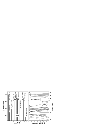
Figure 1: Left: Strength $T^{(1)}_{fi}$ of ten favored hyperfine components $M_{1},\ldots,M_{10}$ of the $(0,1)\rightarrow(4,2)$ one-photon transition line at $B\!=\!0$ (no $\theta$-dependence), labeled with the quantum numbers $(FSJ)$ of the initial and final states. Right: Frequencies of the $\Delta J_{z}\!=\!0$ components of $M_{1},\ldots,M_{10}$ as function of the magnetic field $B$ for $\theta\!=\!0$. The $J_{z}\!=\!0\rightarrow J^{\prime}_{z}\!=\!0$ components of $M_{8}$ and $M_{10}$ (short dotted lines) undergo a very small quadratic shift. The frequencies of the transitions between stretched states in transversal field (dotted lines) have a very small linear shift; their mean is independent of $B$.

Transitions. The probability per unit time for an electric dipole transition between a lower $|i\rangle\!\equiv\!|vLnJ_{z}\rangle$ and upper $\langle f|\!\equiv\!\langle v^{\prime}L^{\prime}n^{\prime}J^{\prime}_{z}|$ states, stimulated by an oscillating electric field ${\mathbf{E}}(t)={\mathbf{E}}\,\cos 2\pi\nu t$ of frequency $\nu$, is (in units $h=1$) $\pi^{2}\delta(\nu\!-\!\nu_{fi})|\langle f|W|i\rangle|^{2}$, where $\nu_{fi}\!=\!\nu_{0}\!+\!\Delta E^{v^{\prime}L^{\prime}n^{\prime}J^{\prime}_{z}}\!-\!\Delta E^{vLnJ_{z}}$, $\nu_{0}\!=\!E^{v^{\prime}L^{\prime}}\!-\!E^{vL}$ is referred to as “central frequency”,  $W\!=\!-{\mathbf{E}}.{\mathbf{d}}$ is the interaction with the electric field, and ${\mathbf{d}}$ is the electric dipole moment operator. The matrix elements $\langle f|W|i\rangle$ are expressed in terms of the reduced matrix elements of ${\mathbf{d}}$ which, in the non-relativistic approximation, do not depend of the spin quantum numbers: $d_{fi}\equiv d_{v^{\prime}L^{\prime},vL}$. Accurate numerical values of $d_{v^{\prime}L^{\prime},vL}$ have been calculated with the variational Coulomb wave functions of Ref. DDBkorobov ; they agree with earlier results of Ref. bunker at the $10^{-3}$ level. Assuming statistical population of the hyperfine states, the observable spectrum of the transition $(v,L)\!\rightarrow\!(v^{\prime},L^{\prime})$ can be put in the form $|{\mathbf{E}}|^{2}\sum_{f,i}\delta(\nu-\nu_{fi})\,T^{(1)}_{fi}(\theta)$, where $\theta$ is the angle between ${\mathbf{B}}$ and ${\mathbf{E}}$, the sum is over all pairs of states $(i,f)$ belonging to the hyperfine structure of the initial and final ro-vibrational states. The number of hyperfine lines may exceed $10^{3}$, but most of them are weak. For magnetic fields $B$ below a few G the spectrum is dominated by the “favored” components corresponding to transitions between states that satisfy $\Delta S\!=\!\Delta F\!=\!0$; the frequencies of the favored transitions lie in a band of width $\sim 100$ MHz around $\nu_{0}$. Fig. 1 illustrates the Zeeman structure of an overtone ro-vibrational transition ($(0,1)\rightarrow(4,2)$), to be discussed further below.

Of interest also are the radio-frequency (RF) magnetic dipole (M1) transitions between spin sub-states of the same $(vL)$ state, stimulated by an oscillating magnetic field ${\mathbf{B}}^{\prime}\cos 2\pi\nu t$. The frequencies $\nu_{fi}$ of the transitions with $\Delta F=\pm 1$ are in the range $700<\nu_{fi}<1100$ MHz, while $\nu_{fi}<200$ MHz for $\Delta F=0$. The explicit expressions of the RF transition probabilities show that they are mainly due to the $({\mathbf{B}}^{\prime}\cdot{\mathbf{S}}_{e})$ term in $V^{\rm mag}$.

The two-photon spectrum may similarly be put in the form $|{\mathbf{E}}|^{4}\sum_{f,i}\delta(\nu\!-\!\nu_{fi}/2)\,T^{(2)}_{fi}(\theta)$. In transverse polarization ($\theta\!=\!\pi/2$) each favored hyperfine component splits into 3 components with $\Delta J_{z}=J^{\prime}_{z}-J_{z}=-2,0,2$ with a typical separation of the order of $\sim 10^{2}$ kHz at $B=0.5$ G; each of these components acquires an additional super-fine structure with separations in the $10^{1}$ kHz range. In a longitudinal magnetic field ($\theta=0$) $\Delta J_{z}=0$, and the lines are “super-fine” split only.

Transitions between stretched states are allowed by selection rules, both as one-photon pure rotational ($v=v^{\prime}$) or ro-vibrational as well as two-photon transitions.

Discussion. At low $B$, the Zeeman shift of the frequency of a single Zeeman component may be estimated using Eq. (1): $\delta\nu_{fi}(B)\approx(h^{\prime}J^{\prime}_{z}-hJ_{z})B+(q^{\prime}-q)B^{2}$. The systematic uncertainty due to the external magnetic field may be minimized by selecting transitions with minimal $\delta\nu_{fi}(B)$. We describe a few concrete transitions, for different cases of assumed experimental spectral resolution.

1: Resolved hyperfine structure, unresolved Zeeman subcomponents. The level of spectroscopic resolution needed for improved measurements of mass ratios is about 10 kHz for an overtone vibrational transition and therefore requires experimental resolution of the hyperfine structure (with typical spacing of several MHz, see Fig. 1), but not necessarily of the Zeeman sublevels.

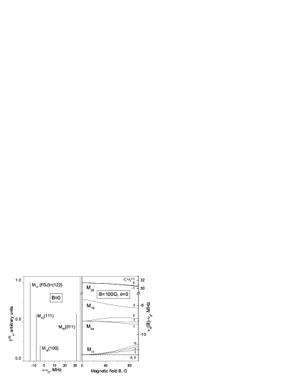
Figure 2: Left: strength $T^{(2)}_{fi}$ of the favored components of the $(0,0)\rightarrow(2,0)$ two-photon transition line at $B\!=\!0$, labelled with the quantum numbers $(FSJ)\!=\!(F^{\prime}S^{\prime}J^{\prime})$. Right: Zeeman shift of the $\Delta J_{z}\!=\!0$ components in external magnetic field $B$. The spectrum is independent of $\theta$. The transition frequencies between stretched states ($J_{z}\!=\!\pm 2$ components of $M_{17}$, dotted line) are independent of $B$.

Among one-photon transition, a favorable case is the triplet of magnetic subcomponents $|vL(FSJ)J_{z}\rangle=|01(010)0\rangle\rightarrow|42(011)J_{z}^{\prime}\rangle$. The $J_{z}\!=\!0\rightarrow J_{z}^{\prime}\!=\!0$ subcomponent (parallel polarization) has a very small quadratic Zeeman shift (-18 Hz at 1 G), while the $J_{z}\!=\!0\rightarrow J_{z}^{\prime}\!=\!\pm 1$ subcomponents (observable in perpendicular polarization) have dominant linear Zeeman shifts of 34.3 and $-$36.3 kHz, respectively, with an intensity-weighted shift of only 290 Hz at 1 G ($1.3\cdot 10^{-12}$ in relative units). If the magnetic field direction is not optimal, the latter value sets the scale of the Zeeman systematic effect. A two-photon transition candidate is the $\theta$-insensitive $|00(011)J_{z}\rangle\rightarrow|20(011)J_{z}\rangle$ triplet (line $M_{20}$ in Fig. 2) with a weighed shift of $-$95 Hz at 1 G $(-8\cdot 10^{-13})$. As fields below 1 G are feasible, such shift values will be well below the current and near-future theoretical uncertainties and thus will not be a limitation in comparisons of theoretical and experimental results.

2: Resolved Zeeman subcomponents: the preferred experimental situation, in which the transition frequencies of individual subcomponents can be measured. Examples of one-photon transitions with very low magnetic field sensitivity include transitions with $J^{\prime}_{z}\!=\!J_{z}\!=\!0$ with eliminated linear and suppressed quadratic dependence on $B$: $|vL(FSJ)J_{z}\rangle\!=\!|01(011)0\rangle\!\rightarrow\!|02(012)0\rangle$ (pure rotational), $|01(112)0\rangle\!\rightarrow\!|32(113)0\rangle$, $|01(010)0\rangle\!\rightarrow\!|42(011)0\rangle$, $|01(012)0\rangle\!\rightarrow\!|42(013)0\rangle$, $|02(012)0\rangle\!\rightarrow\!|43(013)0\rangle$, with sensitivities $\delta\nu(1\mathrm{G})/\nu_{0}\!\approx\!(3,0.1,-0.08,-0.2,-0.2)\cdot 10^{-12}$, respectively. The sensitivity may also be weak in transitions with $\Delta J_{z}\neq 0$, e.g. in $|02(011){-1}\rangle\!\rightarrow\!|43(012){-2}\rangle$ with $|\delta\nu(B)/\nu_{0}|<8\cdot 10^{-13}$ for $B<1\,$G.

One-photon pure rotational or ro-vibrational transitions between stretched states occur as a doublet with purely linear magnetic shift: $\delta\nu_{fi}(B)=\pm(L^{\prime}\,E^{\prime}_{10}-L\,E_{10})B$ for $J_{z}=\pm(L+2)\rightarrow J_{z}^{\prime}=\pm(L^{\prime}+2)$, where $L,E_{10}$ $(L^{\prime},E^{\prime}_{10})$ refer to the initial (final) state, and $|L-L^{\prime}|=1$. This is about $\pm 0.5\,$kHz for $B=1$ G. The mean of the frequencies is strictly independent of $B$ in the adopted approximation. It should be possible to measure each doublet component independently and then compute the average, as in atomic optical clocks.

Fig. 1 gives an example of a one-photon transition, $(0,1)\rightarrow(4,2)$ at $\lambda\approx 1.4\,$$\mu$m. The hyperfine spectrum includes 18 favored lines of which 10 are plotted. While most of them are quite sensitive to the external magnetic field strength, the $J_{z}\!=\!0\rightarrow J_{z}^{\prime}\!=\!0$ subcomponents of $M_{8}$ and $M_{10}$ are weakly sensitive to $B$. Line $M_{10}$ also contains the moderately sensitive doublet mentioned above, and $M_{4}$ contains the stretched states transitions observable at perpendicular polarization only.

Two-photon transitions between stretched states are of metrological interest. In transitions with $L^{\prime}=L\pm 2$ the doublet splitting is of order $\pm 10\,$Hz/G, since $E_{01}$ varies weakly with the vibrational quantum number, and the mean shift is zero. Again, it should be possible to measure each doublet component independently and then compute the mean. For two-photon transitions with $L^{\prime}\!=\!L\!=\!0$ there is no splitting and no shift. Favourable two-photon transitions are $(0,0)\rightarrow(2,0)$ at $2\times 5.362\,\mu$m and $(0,1)\rightarrow(2,1)$ at $2\times 5.368\,\mu$m, which have intermediate states whose detuning is not too large and therefore allow a reasonable excitation strength for realistic laser power from quantum cascade lasers. In addition, the $(0,0)\rightarrow(2,0)$ transition has a particularly simple spectrum, see Fig. 2, since the $L\!=\!0$ states have only four levels and the two-photon transition selection rules bcagnac allow only $\Delta J\!=\!\Delta J_{z}\!=\!0$ transitions. This gives a relatively strong weight to the stretched states transition relative to the sum over all transitions (which are all equally strong). Its frequency is given by a simple expression, see below.

3. Comparison of ab-initio theory and experiment. When spectroscopy of HD⁺ is pursued with the goal of comparison with QED calculations and for a determination of the particle mass ratio, it may be important to determine the central frequency $\nu_{0}$ since in the adopted approximation, unlike the spin corrections, $\nu_{0}$ includes the contribution of QED corrections of order $O(m\alpha^{5})$ and $O(m\alpha^{5}\log\alpha)$. We propose to combine the results of optical pectroscopy between vibrational levels $(v,L)$ and $(v^{\prime},L^{\prime})$ with the results of RF spectroscopy within each of these levels to extract $\nu_{0}$. Indeed, the coefficients of the effective spin Hamiltonian $E_{i}$ and the spin corrections to $E^{vL}$, can be expressed in terms of the frequencies of RF transitions within the hyperfine structure of the $(v,L)$ state (and similar for the $(v^{\prime},L^{\prime})$ state). Since the number $n_{h}$ of linearly independent hyperfine transition frequencies exceeds the number $N_{e}$ of non-vanishing $E_{i}$, the above relations can be resolved for $E_{i}$ only if the radio-frequencies satisfy $N_{h}-N_{e}$ compatibility relations, that may serve to test the experimental accuracy. The value of $\nu_{0}$ is then expressed in terms of spectroscopic data and may be used to test the predictions of few-body bound state QED in next-to-leading orders in $\alpha$. This approach is particularly simple in states with $L\!=\!0$, since the only non-vanishing coefficients are $E_{4}$ and $E_{5}$. Denote the frequencies of the $J_{z}\!=\!0\rightarrow J^{\prime}_{z}\!=\!0$ components at $B=0$ of three RF transitions in the $(v,L=0)$ state as follows: $\nu_{1}=\nu_{v0(111)0,v0(100)0}$, $\nu_{2}=\nu_{v0(122)0,v0(111)0}$ $\nu_{3}=\nu_{v0(100)0,v0(011)0}$, and similarly, by $\nu^{\prime}_{1}\ldots,\nu^{\prime}_{3}$, the corresponding frequencies in the $(v^{\prime},0)$ state. Diagonalizing the hyperfine hamiltonian, we obtain $E_{4}=\nu_{2}+\nu_{3}$, $E_{5}=2\,(\nu_{1}+\nu_{2})/3$, with compatibility relation $\nu_{2}(\nu_{1}+\nu_{2}+\nu_{3})=2\nu_{1}\nu_{3}$ (and similar for the $(v^{\prime},0)$ state). The spin energy of the stretched states is $\Delta E^{v0(122)2}=E_{4}/4+E_{5}/2=\nu_{1}/3+7\nu_{2}/12+\nu_{3}/4$. The transition frequency between stretched states is $\nu_{v0(122)2,v^{\prime}0(122)2}=\nu_{0}+\Delta\nu$, $\Delta\nu=1/3\,(\nu^{\prime}_{1}-\nu_{1})+7/12\,(\nu^{\prime}_{2}-\nu_{2})+(\nu^{\prime}_{3}-\nu_{3})/4$. Thus, $\nu_{0}$ could be obtained by measuring one vibrational transition, and six RF transitions. The sensitivity to magnetic field comes only from $\Delta\nu$, since the Zeeman shift of $\nu_{v0(122)2,v^{\prime}0(122)2}$ is strictly zero in the adopted approximation. For example, $\Delta\nu$ is shifted by only 55 Hz ($5\cdot 10^{-13}$) in the case $v=0,v^{\prime}=2$ at $B=1$ G. This shift value could be taken as a conservative Zeeman uncertainty for $\nu_{0}$, but it could be further reduced by correcting for the magnetic field in the trap; the field could be determined e.g. from a measurement of the Zeeman splitting of an appropriate magnetic-sensitive transition and using the theoretical magnetic sensitivities.

4. Spectroscopic techniques. In order to achieve the spectroscopic resolutions discussed, a Doppler-free technique is required, and two methods appear suitable. Two-photon spectroscopy with counter-propagating beams of an ensemble of cooled, but not strongly confined molecular ions strongly suppresses the first-order Doppler broadening jcbergquist . Second is quantum logic spectroscopy trosenband on a single HD⁺ ion. For both methods, techniques for strongly populating the lower spectroscopic state will be helpful tschneider .

Summary. By evaluating the Zeeman effect for all experimentally relevant spectroscopies of HD⁺ we have shown that it will not be a limiting factor for the experimental accuracy if appropriate transitions and spectroscopic technique are selected. This is of particular relevance to the possible use of HD⁺ for setting limits to a hypothetical time-dependence of particle mass ratios, where a relative accuracy of $10^{-16}$ is desired. For the determination of the ratio of electron to reduced nuclear mass by comparison of ab initio QED calculations and experimental frequencies, it is advantageous to determine the central transition frequencies $\nu_{0}$ since the uncertainties related to particle magnetic moments and nuclear electromagnetic structure will be significantly suppressed. We have shown how this can be achieved by combining two-photon and RF spectroscopy of states with low magnetic sensitivity, the latter feature not being affected by the higher-order relativistic mass and anisotropy corrections.

Other systematic shifts, such as light, blackbody radiation and Stark shifts are currently being analyzed.

Acknowledgments The work was partly supported by Grant 02-288 of the Bulgarian Science Fund (D.B.) and the Russian Foundation for Basic Research under Grant No. 08-02-00341 (V.I.K.). D.B. and V.I.K also acknowledge the support from a JINR grant for the joint research of BLTP-JINR and INRNE-BAS. The work of S.S. was supported by DFG project Schi 431/11-1.

Table 1: Numerical values of the coefficients $h^{vLn}$ (upper line, in kHz/G) and $q^{vLnJ_{z}},J_{z}=0$ (lower line, in kHz/G²) in the weighed least-square approximation (1) of the dependence of the Zeeman corrections to the hyperfine energy levels on the magnetic field $B$ for the ro-vibrational states of the HD⁺ ion with $L\leq 4$ and $v\leq 4$. The relative inaccuracy of the approximation does not exceed $5.10^{-7}$ for $B<1$ G, except for the $F=1$ components of the states with $L=1$ where accuracy better than $10^{-5}$ can only be achieved with higher degree polynomial approximation.

	$(F,S)=(0,1)$			$(1,0)$	$(1,1)$			$(1,2)$
$vL$	$J\!=\!L\!+\!1$	$L$	$L\!-\!1$	$L$	$L\!+\!1$	$L$	$L\!-\!1$	$L\!+\!2$	$L\!+\!1$	$L$	$L\!-\!1$	$L\!-\!2$
00	-218.820			0.000	917.397			699.233
	-2.074			-17.657	14.784			4.947
10	-218.835			0.000	917.411			699.233
	-2.122			-18.071	15.130			5.063
20	-218.851			0.000	917.428			699.233
	-2.170			-18.475	15.468			5.176
30	-218.871			0.000	917.448			699.233
	-2.217			-18.869	15.798			5.287
40	-218.894			0.000	917.470			699.233
	-2.262			-19.251	16.119			5.394
01	-129.368	-148.704	0.000	-473.172	466.638	821.918	0.000	465.376	595.729	1197.227
	-4.988	-2.940	1.743	-12.606	8.611	-95.776	92.665	-95.865	106.989	2.167
11	-128.783	-147.464	0.000	-459.754	466.337	809.370	0.000	465.291	595.691	1195.121
	-5.222	-3.121	2.015	-13.127	9.133	-99.725	96.462	-104.234	115.802	2.019
21	-128.183	-146.200	0.000	-445.608	466.036	796.288	0.000	465.198	595.666	1192.796
	-5.470	-3.317	2.318	-13.657	9.694	-103.890	100.450	-113.351	125.380	1.843
31	-127.569	-144.909	0.000	-430.712	465.734	782.670	0.000	465.096	595.651	1190.231
	-5.735	-3.529	2.658	-14.193	10.301	-108.308	104.657	-123.282	135.795	1.635
41	-126.934	-143.585	0.000	-415.040	465.434	768.518	0.000	464.990	595.642	1187.400
	-6.018	-3.762	3.042	-14.736	10.961	-113.021	109.119	-134.081	147.104	1.391
02	-100.293	-80.709	24.335	-364.548	307.231	442.688	-650.959	349.337	374.520	466.911	624.618	0.000
	-4.198	-2.932	0.904	-11.457	7.212	32.570	-35.737	37.105	-17.480	7.061	25.264	-38.314
12	-99.490	-79.360	27.011	-357.541	307.093	437.197	-646.350	349.339	373.864	464.072	617.290	0.000
	-4.387	-3.058	1.076	-11.972	7.650	35.119	-38.324	38.907	-18.322	7.352	26.707	-40.748
22	-98.667	-77.979	29.748	-350.004	306.960	431.260	-641.463	349.342	373.184	461.119	609.615	0.000
	-4.587	-3.190	1.268	-12.503	8.122	37.889	-41.147	40.830	-19.226	7.658	28.256	-43.371
32	-97.821	-76.563	32.551	-341.885	306.832	424.836	-636.285	349.345	372.478	458.041	601.573	0.000
	-4.799	-3.329	1.484	-13.047	8.633	40.913	-44.244	42.891	-20.201	7.981	29.928	-46.210
42	-96.945	-75.101	35.443	-333.120	306.715	417.886	-630.789	349.353	371.747	454.830	593.142	0.000
	-5.026	-3.478	1.727	-13.606	9.190	44.230	-47.658	45.113	-21.260	8.326	31.739	-49.298
03	-85.696	-63.510	2.629	-296.799	225.824	311.507	-423.624	279.364	278.044	279.838	186.045	-700.466
	-3.705	-2.584	0.060	-9.894	5.759	15.852	-18.897	20.502	0.673	6.205	8.318	-22.289
13	-84.790	-62.138	4.836	-292.840	225.798	308.857	-420.847	279.367	277.175	277.177	181.073	-700.471
	-3.865	-2.675	0.167	-10.377	6.114	17.059	-20.106	21.586	0.636	6.430	8.663	-23.633
23	-83.861	-60.733	7.093	-288.510	225.782	305.901	-417.911	279.371	276.272	274.419	175.891	-700.478
	-4.033	-2.770	0.289	-10.879	6.499	18.360	-21.414	22.745	0.590	6.664	9.027	-25.078
33	-82.904	-59.289	9.408	-283.760	225.777	302.597	-414.802	279.375	275.335	271.554	170.482	-700.484
	-4.210	-2.867	0.427	-11.402	6.917	19.767	-22.835	23.991	0.532	6.908	9.412	-26.640
43	-81.913	-57.797	11.796	-278.525	225.789	298.905	-411.500	279.385	274.363	268.576	164.836	-700.477
	-4.399	-2.970	0.586	-11.947	7.374	21.296	-24.388	25.336	0.460	7.163	9.824	-28.336
04	-76.724	-56.329	-8.945	-248.212	176.961	237.613	-317.629	232.709	224.638	204.655	91.646	-467.118
	-3.387	-2.407	-0.434	-8.642	4.784	10.241	-13.379	14.907	5.129	5.664	3.631	-16.106
14	-75.767	-54.959	-6.945	-245.779	176.976	236.409	-315.688	232.713	223.678	202.075	87.721	-467.114
	-3.527	-2.483	-0.363	-9.083	5.079	11.062	-14.192	15.714	5.315	5.842	3.694	-17.059
24	-74.783	-53.554	-4.898	-243.092	177.005	235.011	-313.627	232.717	222.678	199.401	83.629	-467.110
	-3.674	-2.560	-0.280	-9.546	5.399	11.949	-15.067	16.577	5.507	6.025	3.754	-18.084
34	-73.770	-52.109	-2.797	-240.113	177.049	233.388	-311.433	232.722	221.635	196.626	79.356	-467.104
	-3.828	-2.639	-0.184	-10.032	5.747	12.908	-16.014	17.506	5.704	6.212	3.812	-19.190
44	-72.720	-50.616	-0.632	-236.790	177.114	231.504	-309.090	232.731	220.549	193.743	74.889	-467.090
	-3.993	-2.720	-0.072	-10.545	6.130	13.949	-17.046	18.510	5.907	6.404	3.867	-20.391

References

- (1) U. Fröhlich, et al., Lect. Notes in Phys. 648, 297 (2004).
- (2) S. Schiller and V. Korobov, Phys.Rev.A71, 32505 (2005).
- (3) J.C.J.Koelemeij et al., Phys.Rev.Lett. 98, 173002 (2007).
- (4) H. Müller, et al., Phys. Rev. D 70, 076004 (2004).
- (5) M. Kajita, Phys. Rev. A 77, 012511 (2008);
- (6) C. Chin, V.V. Flambaum, M.G. Kozlov, New J. Phys. 11, 055048 (2009).
- (7) D. DeMille, et al. Phys. Rev. Lett. 100, 043202 (2008)
- (8) T. Zelevinsky, S. Kotochigova, J. Ye, Phys. Rev. Lett. 100, 043201 (2008)
- (9) V.I. Korobov. Phys. Rev. A 77, 022509 (2008).
- (10) P. Blythe et al., Phys. Rev. Lett. 95, 183002 (2005).
- (11) T. Schneider, et al., Nature Physics 6, 275 (2010).
- (12) J.-Ph. Karr, S. Kilic, and L. Hilico, J. Phys. B 38, 853 (2005).
- (13) D.Bakalov, V.I.Korobov, S.Schiller, Phys. Rev. Lett. 97, 243001 (2006).
- (14) B. Roth, et al., Lect. Notes in Phys. 745, 205 (2008).
- (15) R.A.Hegstrom, Phys. Rev. A 19, 17 (1979).
- (16) V. I. Korobov, Phys. Rev. A 74 (2006) 052506.
- (17) E. A. Colbourn and P. R. Bunker, J. Mol. Spectrosc. 63, 155 (1976).
- (18) B. Cagnac, G. Grynberg, and F. Biraben, J. Phys. (Paris) 34, 845 (1973).
- (19) J.C. Bergquist, et al., Phys. Rev. Lett. 55, 1567 (1985)
- (20) T. Rosenband et al., Phys. Rev. Lett. 98, 220801 (2007); P. O. Schmidt et al., Science 309, 749 (2005).
- (21) A. Carrington, et al., Mol. Phys. 72, 735 (1991).
- (22) C.A. Leach and R.E. Moss, Annu. Rev. Phys. Chem. 46, 55 (1995).