On the Sensitivity of L/E Analysis of Super-Kamiokande Atmospheric Neutrino Data to Neutrino Oscillation Part 1

Abstract

It is said that the finding of the maximum oscillation in neutrino oscillation by Super-Kamiokande is one of the major achievements of the SK. In present paper, we examine the assumption made by Super-Kamiokande Collaboration that the direction of the incident neutrino is approximately the same as that of the produced lepton, which is the cornerstone in their $L/E$ analysis and we find this approximation does not hold even approximately. In the Part 2 of the subsequent paper, we apply the results from Figures 12, 13 and 14 to $L/E$ analysis and conclude that one cannot obtain the maximum oscillation in $L/E$ analysis which shows strongly the oscillation pattern from the neutrino oscillation.

1 Introduction

According to the results obtained from the Super-Kamio- kande Experiments on atmospheric neutrinos, it is said that oscillation phenomena have been found between two neutrinos, $\nu_{\mu}$and $\nu_{\tau}$. Published reports on the confirmation to the oscillation between the neutrinos, $\nu_{\mu}$and $\nu_{\tau}$, and the history foregoing these experiments will be critically reviewed and details are in the following:

• During 1980’s Kamiokande and IMB observed smaller atmospheric neutrino flux ratio $\nu_{\mu}/\nu_{e}$ than the predicted value Hirata .

• Kamiokande found anomaly in the zenith angle distribution Hatakeyama .

• Super-Kamiokande found $\nu_{\mu}$-$\nu_{\tau}$ oscillation Kajita2 and
  Soudan2 and MACRO confirmed the Super-Kamiokande result Mann .

• K2K, the first accelerator-based long baseline experiment, confirmed atmospheric neutrino oscillationK2K .

• MINOS’s precision measurement gives the consistent results with Super-Kamiokande onesMINOS .

It is well known that Super-Kamiokande Collaboration examined all possible types of the neutrino events, such as, say, Sub-GeV e-like, Multi-GeV e-like, Sub-GeV $\mu$-like, Multi-GeV $\mu$-like, Multi-ring Sub-GeV $\mu$-like, Multi-ring Multi-GeV $\mu$-like, PC, Upward Stopping Muon Events and Upward Through Going Muon Events. In other words, all possible interactions by neutrinos, such as, elastic and quasielastic scattering, single-meson production and deep scattering are considered in their analyses. Furthermore, all topologically different types of neutrino events lead to the unified numerical oscillation parameters, say, $\Delta m^{2}=2.4\times 10^{-3}\rm{eV^{2}}$ and $sin^{2}2\theta=1.0$ Ashie2 .

However, these parameters are obtained from the analysis of the zenith angle distribution of the incident neutrinos which are based on the survival probability of a given flavor( see Eq.(7)). The most important result among the achievements on neutrino oscillation made by Super-
Kamiokande Collaboration is the finding of the maximum oscillation in neutrino oscillation, because it is the ultimate result in the sense that they observe the oscillation pattern itself directly in neutrino oscillation.

Taking account of all factors mentioned above, it is natural that the majority believes the finding of the $\mu-\tau$ neutrino oscillation by Super-Kamiokande Collaboration.

However, it should be emphasized strongly that Super-Kamiokande Collaboration put the fundamental assumption in all possible analyses of the atmospheric neutrino oscillation which is never self-evident and should be carefully examined. This assumption is that the directions of the incident neutrinos are approximately the same as those of emitted leptons.

In order to avoid any misunderstanding toward the SK assumption on the direction, we reproduce this assumption from the original SK papers and their related papers in italic.

[A] Kajita and Totsuka Kajita1 state :

”However, the direction of the neutrino must be estimated from the reconstructed direction of the products of the neutrino interaction. In water Cheren-kov detectors, the direction of an observed lepton is assumed to be the direction of the neutrino. Fig.11 and Fig.12 show the estimated correlation angle between neutrinos and leptons as a function of lepton momentum. At energies below 400 MeV/c, the lepton direction has little correlation with the neutrino direction. The correlation angle becomes smaller with increasing lepton momentum. Therefore, the zenith angle dependence of the flux as a consequence of neutrino oscillation is largely washed out below 400 MeV/c lepton momentum. With increasing momentum, the effect can be seen more clearly.”

[B] Ishitsuka Ishitsuka states:

” 8.4 Reconstruction of $L_{\nu}$

Flight length of neutrino is determined from the neutrino incident zenith angle, although the energy and the flavor are also involved. First, the direction of neutrino is estimated for each sample by a different way. Then, the neutrino flight lenght is calclulated from the zenith angle of the reconstructed direction.

8.4.1 Reconstruction of Neutrino Direction

FC Single-ring Sample

The direction of neutrino for FC single-ring sample is simply assumed to be the same as the reconstructed direction of muon. Zenith angle of neutrino is reconstructed as follows:

$$\hskip 56.9055pt\cos\Theta^{rec}_{\nu}=\cos\Theta_{\mu}\hskip 56.9055pt(8.17)$$

,where $\cos\Theta^{rec}_{\nu}$ and $\cos\Theta_{\mu}$ are cosine of the reconstructed zenith angle of neutrino and muon, respectively.”

[C] Jung, Kajita et al. Jung state :

”At neutrino energies of more than a few hundred MeV, the direction of the reconstructed lepton approximately represents the direction of the original neutrino. Hence, for detectors near the surface of the Earth, the neutrino flight distance is a function of the zenith direction of the lepton. Any effects, such as neutrino oscillations, that are a function of the neutrino flight distance will be manifest in the lepton zenith angle distributions.”

Hereafter, we call the fundamental assumption by the Super-Kamiokande Experiment simply as the SK assumption on the direction.

Among various types of the neutrino events analyzed by Super-Kamiokande, the most important events are single ring muon(electron) events which are generated in the detector and terminate in it, because these events give more essential physical quantities for clear interpretation on neutrino oscillation, namely, the kinds of the neutrino, the transferred energies and the directions of the produced leptons. These single ring muon events are generated from the quasi elastic scattering (QEL). If the existence of neutrino oscillation is verified surely in the analyses of single ring muon events among Fully Contained Events under the SK assumption on the direction, then we can expect the corroboration of the oscillation in the analyses of other types of the interaction with less accuracy. Therefore, the SK assumption on the direction should be carefully examined in the analysis of single ring events due to QEL among Fully Contained Events.

Our paper is organized as follows. In section 2, we treat the differential cross section for QEL in the stochastic manner as exactly as possible and obtain the zenith angle distributions of the emitted leptons, $\cos\theta_{\mu}$, for given neutrinos with definite zenith angles, taking account of the azimuthal angles of the emitted leptons in QEL. As a result of it, we show that the SK assumption on the direction does not hold any more for the incident neutrinos with smaller energies. In section 3, we examine the SK assumption on the direction in the light of $L_{\nu}$ and $L_{\mu}$ and reach the same conclusion obtained in the section 2, as it must be. In section 4, we examine all possible choices of combination of $L$ and $E$, namely, $L_{\nu}/E_{\nu}$, $L_{\nu}/E_{\mu}$, $L_{\mu}/E_{\nu}$, $L_{\mu}/E_{\mu}$, in $L/E$ analysis and show that the maximum oscillation can be realized in the combination of $L_{\nu}/E_{\nu}$, as it must be. In section 5, we compare our results obtained from the numerical experiments with real observation obtained by Super-Kamiokande Collaboration. In section 6, we conclude that SK cannot observe the maximum oscillation in their $L_{\mu}/E_{\nu}$ analysis.

Here, we designate the minimum extrema in $L/E$ distribution for neutrino oscillation as the maximum oscillation by the terminology already utilized in the Super-Kamiokande Collaboration Ashie1 .

2 Single Ring Events among Fully Contained Events which are Produced by Quasi Elastic Scsattering.

2.1 Differential cross section of quasi elastic scattering and influence over various quantities concerned

As stated in Introduction, the finding of the observation of the maximum oscillation in the $L/E$ analysis is the ultimate verification of the finding of the neutrino oscillation by Super-Kamiokande. For the examination of the Super-Kamiokande’s assertion, we analyze the $L/E$ distribution of the single ring events among Fully Contained Events.

In order to examine the validity of the SK assumption on the direction, we consider the single ring events due to the following quasi elastic scattering(QEL):

$$\nu_{e}+n\longrightarrow p+e^{-}$$

$$\nu_{\mu}+n\longrightarrow p+\mu^{-}$$

$$\bar{\nu}_{e}+p\longrightarrow n+e^{+}$$ (1)

$$\bar{\nu}_{\mu}+p\longrightarrow n+\mu^{+},$$

The differential cross section for QEL is given as follows r4 .

$$\frac{{\rm d}\sigma_{\ell(\bar{\ell})}(E_{\nu(\bar{\nu})})}{{\rm d}Q^{2}}=\frac{G_{F}^{2}{\rm cos}^{2}\theta_{C}}{8\pi E_{\nu(\bar{\nu})}^{2}}\Biggl{\{}A(Q^{2})\pm B(Q^{2})\biggl{[}\frac{s-u}{M^{2}}\biggr{]}+$$

$$C(Q^{2})\biggl{[}\frac{s-u}{M^{2}}\biggr{]}^{2}\Biggr{\}},$$ (2)

where

$$A(Q^{2}) = \frac{Q^{2}}{4}\Biggl{[}f^{2}_{1}\biggl{(}\frac{Q^{2}}{M^{2}}-4\biggr{)}+f_{1}f_{2}\frac{4Q^{2}}{M^{2}}$$

$$+f_{2}^{2}\biggl{(}\frac{Q^{2}}{M^{2}}-\frac{Q^{4}}{4M^{4}}\biggr{)}+g_{1}^{2}\biggl{(}4+\frac{Q^{2}}{M^{2}}\biggl{)}\Biggr{]},$$

$$B(Q^{2}) = (f_{1}+f_{2})g_{1}Q^{2},$$

$$C(Q^{2}) = \frac{M^{2}}{4}\biggl{(}f^{2}_{1}+f^{2}_{2}\frac{Q^{2}}{4M^{2}}+g_{1}^{2}\biggr{)}.$$

The signs $+$ and $-$ refer to $\nu_{\mu(e)}$ and $\bar{\nu}_{\mu(e)}$ for charged current (c.c.) interactions, respectively. The $Q^{2}$ denotes the four momentum transfer between the incident neutrino and the charged lepton. Details of other symbols are given in r4 .

The relation among $Q^{2}$, $E_{\nu(\bar{\nu})}$, the energy of the incident neutrino, $E_{\ell}$, the energy of the emitted charged lepton (muon or electron or their anti-particles) and $\theta_{\rm s}$, the scattering angle of the emitted lepton, is given as

$$Q^{2}=2E_{\nu(\bar{\nu})}E_{\ell}(1-{\rm cos}\theta_{\rm s}).$$ (3)

Also, the energy of the emitted lepton is given by

$$E_{\ell}=E_{\nu(\bar{\nu})}-\frac{Q^{2}}{2M}.$$ (4)

Now, let us examine the magnitude of the scattering angle of the emitted lepton in a quantitative way, as this plays a decisive role in determining the accuracy of the direction of the incident neutrino, which is directly related to the reliability of the zenith angle distribution of single ring muon (electron) events in the Super-Kamiokande Experiment.

By using Eqs. (2) to (4), we obtain the distribution function for the scattering angle of the emitted leptons and the related quantities by a Monte Carlo method. The procedure for determining the scattering angle for a given energy of the incident neutrino is described in Appendix A. Figure 1 shows this relation for muon, from which we can easily understand that the scattering angle $\theta_{\rm s}$ of the emitted lepton ( muon here ) cannot be neglected. For a quantitative examination of the scattering angle, we construct the distribution function for ${\theta_{\rm s}}$ of the emitted lepton from Eqs. (2) to (4) by using the Monte Carlo method.

Figure 2 gives the distribution function for $\theta_{\rm s}$ of the muon produced in the muon neutrino interaction. It can be seen that the muons produced from lower energy neutrinos are scattered over wider angles and that a considerable part of them are scattered even in backward directions. Similar results are obtained for anti-muon neutrinos, electron neutrinos and anti-electron neutrinos.

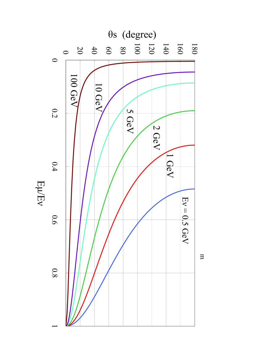
Figure 1: Relation between the energy of the muon and its scattering angle for different incident muon neutrino energies, 0.5, 1, 2, 5, 10 and 100 GeV.

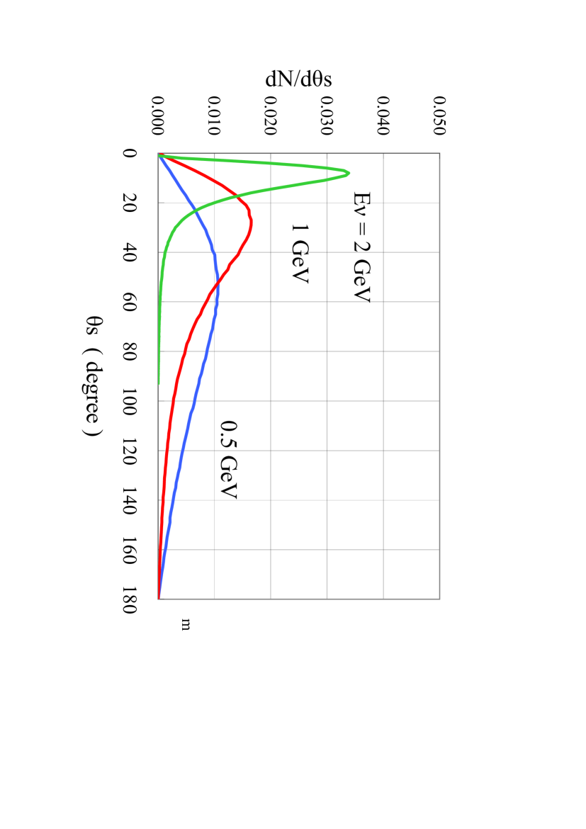
Figure 2: Distribution functions for the scattering angle of the muon for muon-neutrino with incident energies, 0.5 , 1.0 and 2 GeV. Each curve is obtained by the Monte Carlo method (one million sampling per each curve).

Also, in a similar manner, we obtain not only the distribution function for the scattering angle of the charged leptons, but also their average values $<\theta_{\rm s}>$ and their standard deviations $\sigma_{\rm s}$. Table 1 shows them for muon neutrinos, anti-muon neutrinos, electron neutrinos and anti-electron neutrinos. From Table 1, it seems to be clear that the scattering angles could not be neglected, taking account of the fact that the frequency of the neutrino events with smaller energies is far larger than that of the neutrino events with larger energies due to high steep of the neutrino energy spectrum. However, Super-Kamiokande Collaboration assume that the direction of the neutrino is approximately the same as that of the emitted lepton even for the neutrino events with smaller energies, as cited in the three passages mentioned above Kajita1 , Ishitsuka ,Jung . However, it has never been verified by Super-Kamiokande Collaboration.

Table 1: The average values $<\theta_{\rm s}>$ for scattering angle of the emitted charged leptons and their standard deviations $\sigma_{\rm s}$ for various primary neutrino energies $E_{\nu(\bar{\nu})}$.

$E_{\nu(\bar{\nu})}$ (GeV)	angle	$\nu_{\mu(\bar{\mu})}$	$\bar{\nu}_{\mu(\bar{\mu})}$	$\nu_{e}$	$\bar{\nu_{e}}$
	(degree)
0.2	$<\theta_{\mathrm{s}}>$	89.86	67.29	89.74	67.47
	$\sigma_{\mathrm{s}}$	38.63	36.39	38.65	36.45
0.5	$<\theta_{\mathrm{s}}>$	72.17	50.71	72.12	50.78
	$\sigma_{\mathrm{s}}$	37.08	32.79	37.08	32.82
1	$<\theta_{\mathrm{s}}>$	48.44	36.00	48.42	36.01
	$\sigma_{\mathrm{s}}$	32.07	27.05	32.06	27.05
2	$<\theta_{\mathrm{s}}>$	25.84	20.20	25.84	20.20
	$\sigma_{\mathrm{s}}$	21.40	17.04	21.40	17.04
5	$<\theta_{\mathrm{s}}>$	8.84	7.87	8.84	7.87
	$\sigma_{\mathrm{s}}$	8.01	7.33	8.01	7.33
10	$<\theta_{\mathrm{s}}>$	4.14	3.82	4.14	3.82
	$\sigma_{\mathrm{s}}$	3.71	3.22	3.71	3.22
100	$<\theta_{\mathrm{s}}>$	0.38	0.39	0.38	0.39
	$\sigma_{\mathrm{s}}$	0.23	0.24	0.23	0.24

2.2 Influence of azimuthal angle in QEL over the zenith angle of single ring events

In the present subsection, we examine the effect of the azimuthal angles, $\phi$, of the emitted leptons over their own zenith angles, $\theta_{\mu(\bar{\mu}))}$, for given zenith angles of the incident neutrinos, $\theta_{\nu(\bar{\nu}))}$ in QEL, which was not be considered in the detector simulation carried by Super-Kamiokande Collaboration . The influence of this effect over the zenith angle cannot be neglected particularly in horizontal-like neutrino events.

For three typical cases (vertical, horizontal and diagonal), Figure 3 gives a schematic representation of the relationship between, $\theta_{\nu(\bar{\nu})}$, the zenith angle of the incident neutrino, and ( $\theta_{\rm s}$, $\phi$), a pair of scattering angle of the emitted lepton and its azimuthal angle.

From Figure 3-a, it can been seen that the zenith angle $\theta_{\mu(\bar{\mu})}$ of the emitted lepton is not influenced by its $\phi$ in the vertical incidence of the neutrinos $(\theta_{\nu(\bar{\nu})}=0^{\rm o})$, as it must be. From Figure 3-b, however, it is obvious that the influence of $\phi$ of the emitted leptons on their own zenith angle is the strongest in the case of horizontal incidence of the neutrino $(\theta_{\nu(\bar{\nu})}=90^{\rm o})$. Namely, one half of the emitted leptons are recognized as upward going, while the other half is classified as downward going ones. The diagonal case ( $\theta_{\nu(\bar{\nu})}=43^{\rm o}$) is intermediate between the vertical and the horizontal. In the following, we examine the cases for vertical, horizontal and diagonal incidence of the neutrinos with different energies, say, $E_{\nu(\bar{\nu})}=0.5$ GeV, $E_{\nu(\bar{\nu})}=1$ GeV and $E_{\nu(\bar{\nu})}=5$ GeV, as the typical cases.

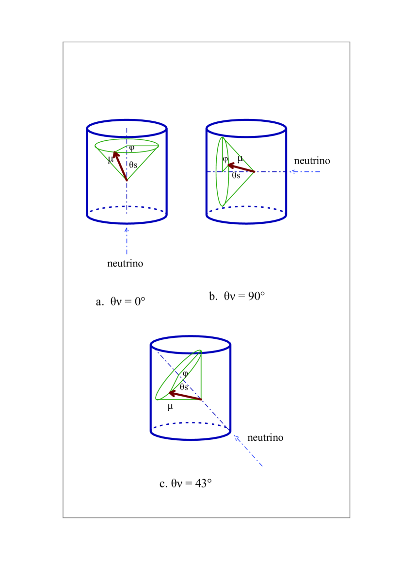
Figure 3: Schematic view of the zenith angles of the charged muons for different zenith angles of the incident neutrinos, focusing on their azimuthal angles.

2.3 Dependence of the spreads of the zenith angle for the emitted leptons on the energies of the emitted leptons for different incident directions of the neutrinos with different energies

The detailed procedure for the Monte Carlo simulation is described in Appendix A. We give the scatter plots between the fractional energies of the emitted muons and their zenith angle for a definite zenith angle of the incident neutrino with different energies in Figures 6 to 6. In Figure 6, we give the scatter plots for vertically incident neutrinos with different energies 0.5, 1 and 5 GeV. In this case, the relations between the emitted energies of the muons and their zenith angles are unique, which comes from the definition of the zenith angle of the emitted lepton. However, the densities (frequencies of the event number) along each curves are different in position to position and depend on the energies of the incident neutrinos. Generally speaking, densities along the curves become greater toward $\cos\theta_{\mu(\bar{\mu})}=1$. In this case, $\cos\theta_{\mu(\bar{\mu})}$ is never influenced by the azimuthal angel in the scattering by the definition .

On the contrast, it is shown in Figure 6 that the horizontally incident neutrinos give the widest zenith angle distributions for the emitted muons with the same fractional energies due to the effect of the azimuthal angles. The lower the energies of the incident neutrinos are, the wider the spreads of the scattering angles of emitted muons $\theta_{\mu}$ become, which leads to wider zenith angle distributions for the emitted muons. As easily understood from Figure 6, the diagonally incident neutrinos give the intermediate zenith angle distributions for the emitted muons between those for vertically incident neutrinos and those for horizontally incident neutrinos.

(a)                                                (b)                                                (c)

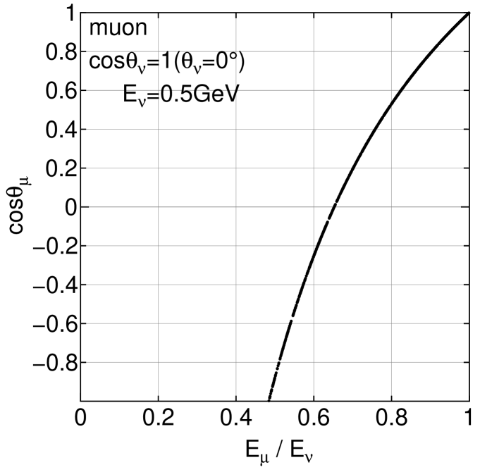
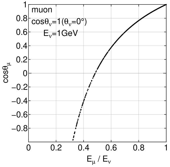
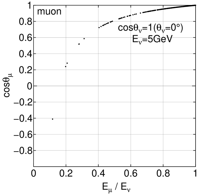
Figure 4: The scatter plots between the fractional energies of the produced muons and their zenith angles for vertically incident muon neutrinos with 0.5 GeV, 1 GeV and 5 GeV, respectively. The sampling number is 1000 for each case.

(a)                                                (b)                                                (c)

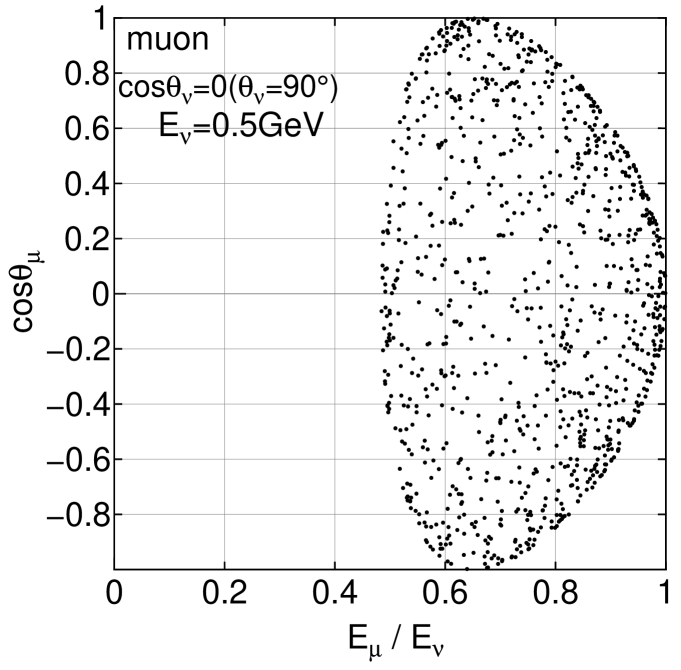
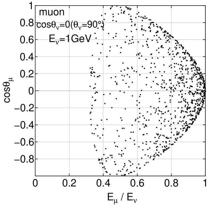
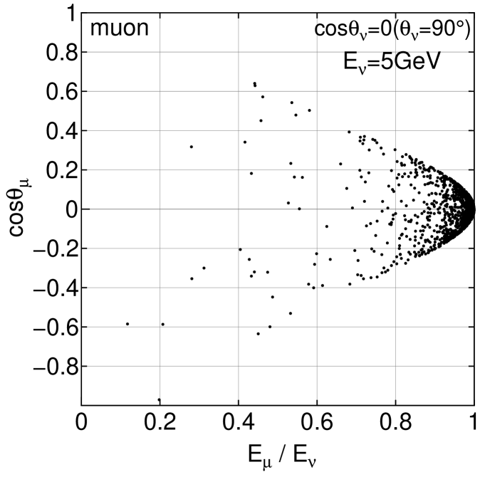
Figure 5: The scatter plots between the fractional energies of the produced muons and their zenith angles for horizontally incident muon neutrinos with 0.5 GeV, 1 GeV and 5 GeV, respectively. The sampling number is 1000 for each case.

(a)                                                (b)                                                (c)

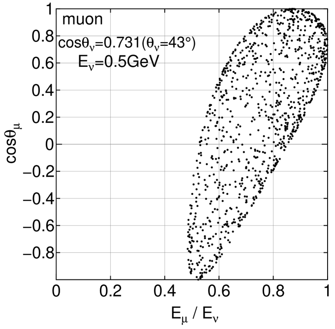
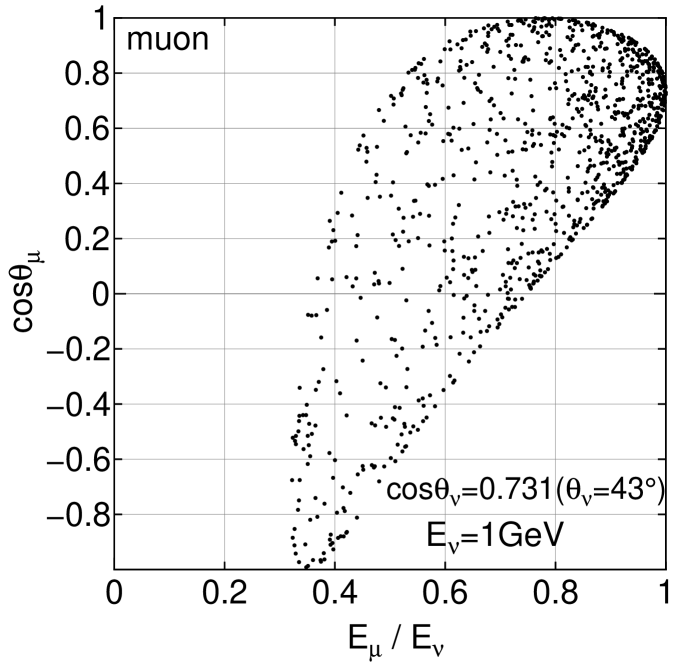
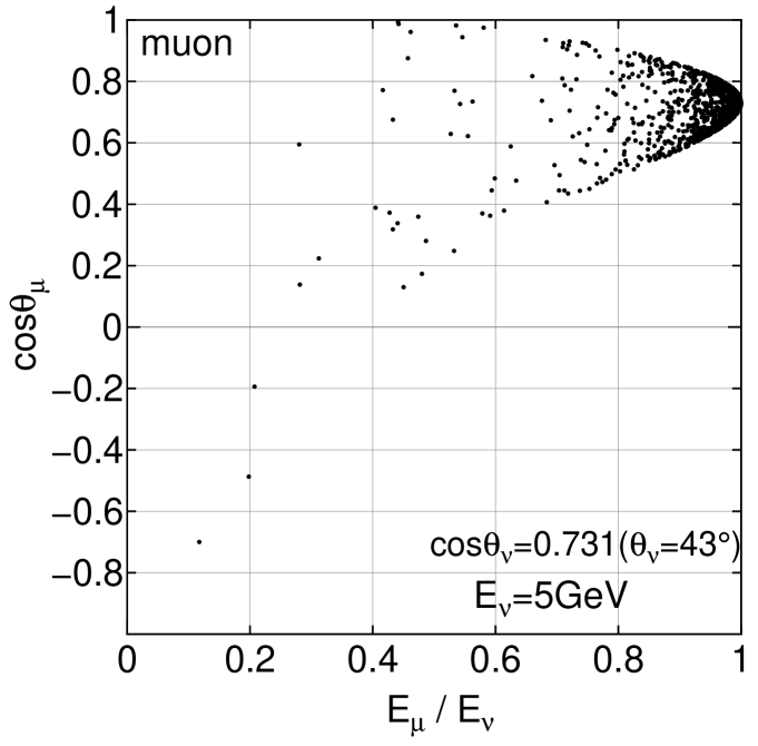
Figure 6: The scatter plots between the fractional energies of the produced muons and their zenith angles for diagonally incident muon neutrinos with 0.5 GeV, 1 GeV and 5 GeV, respectively. The sampling number is 1000 for each case.

(a)                                                (b)                                                (c)

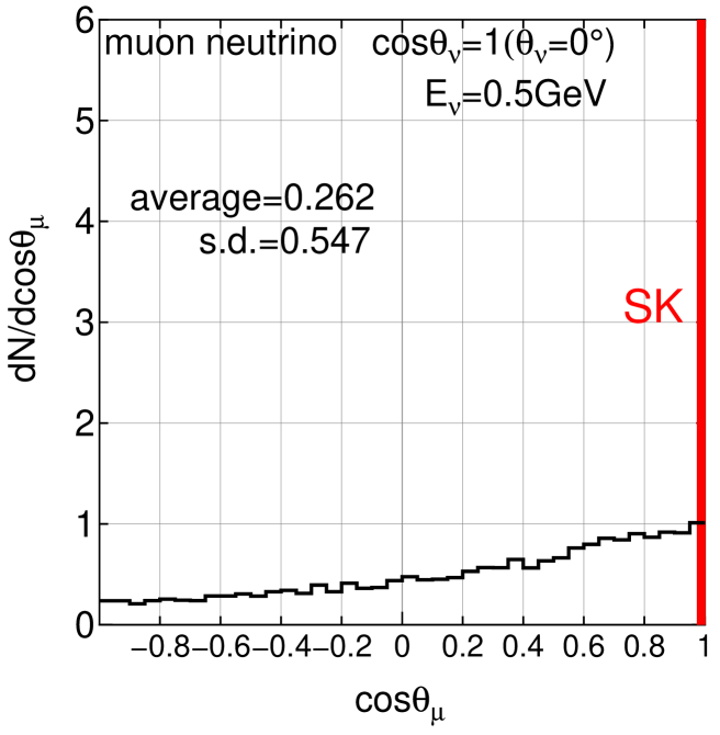
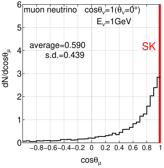
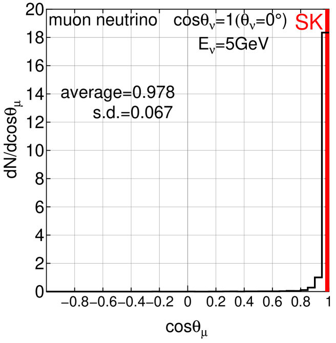
Figure 7: Zenith angle distribution of the muon for the vertically incident muon neutrino with 0.5 GeV, 1 GeV and 5 GeV, respectively. The sampling number is 10000 for each case. SK stands for the corresponding ones under the SK assumption.

(a)                                                (b)                                                (c)

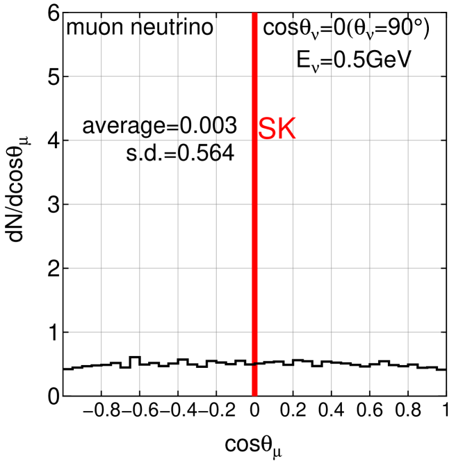
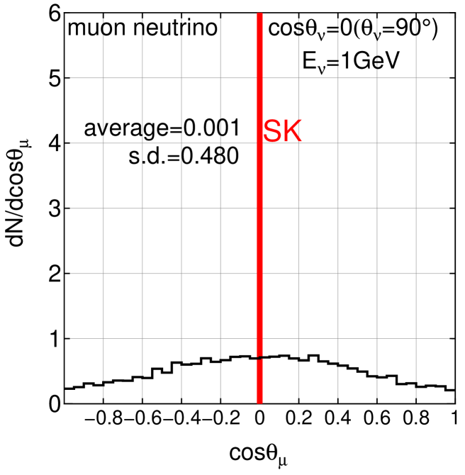
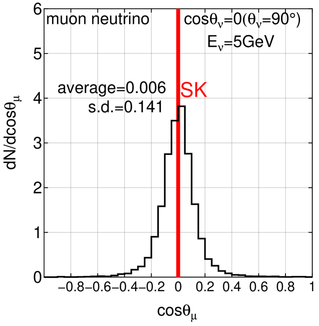
Figure 8: Zenith angle distribution of the muon for the horizontally incident muon neutrino with 0.5 GeV, 1 GeV and 5 GeV, respectively. The sampling number is 10000 for each case. SK stands for the corresponding ones under the SK assumption.

(a)                                                (b)                                                (c)

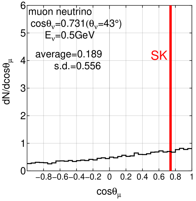
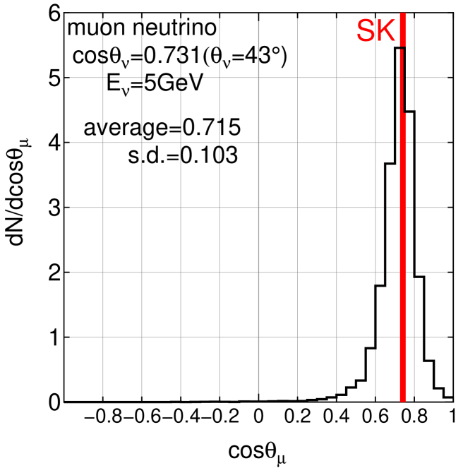
Figure 9: Zenith angle distribution of the muon for the diagonally incident muon neutrino with 0.5 GeV, 1 GeV and 5 GeV, respectively. The sampling number is 10000 for each case. SK stands for the corresponding ones under the SK assumption.

In Figures 9 to 9, we express Figures 6 to 6 in a different way. We sum up muon events with different emitted energies for given zenith angles. As the result of it, we obtain frequency distribution of the neutrino events as a function of $cos\theta_{\mu}$ for different incident directions and different incident energies of neutrinos.

In Figures 9(a) to 9(c), we give the zenith angle distributions of the emitted muons for the case of vertically incident neutrinos with different energies, say, $E_{\nu}=$ 0.5, 1 and 5 GeV.

Comparing the case for 0.5 GeV with that for 5 GeV, we understand the big contrast between them as for the zenith angle distribution. The scattering angle of the emitted muon for 5 GeV neutrino is relatively small (See, Table 1), so that the emitted muons keep roughly the same direction as their original neutrinos. In this case, the effect of their azimuthal angle on the zenith angle is also smaller. However, in the case for 0.5 GeV which is the dominant energy for single ring muon events in the Super-Kamiokande, there is even a possibility for the emitted muon to be emitted in the backward direction due to the larger angle scattering, the effect of which is enhanced by their azimuthal angle.

The most frequent occurrence in the backward direction of the emitted muon appears in the horizontally incident neutrino as shown in Figs. 8(a) to 8(c). In this case, the zenith angle distribution of the emitted muon should be symmetrical with regard to the horizontal direction. Comparing the case for 5 GeV with those both for $\sim$0.5 GeV and for $\sim$1 GeV, even 1 GeV incident neutrinos lose almost the original sense of the incidence if we measure it by the zenith angle of the emitted muon. Figures 9(a) to 9(c) for the diagonally incident neutrinos tell us that the situation for diagonal case lies between the case for the vertically incident neutrinos and that for horizontally incident ones. SK in the figures denotes the SK assumption on the direction of incident neutrinos. From the Figures 9(a) to 9(c), it is clear that the scattering angles of emitted muons influence their zenith angles, which is enhanced by their azimuthal angles, particularly for more inclined directions of the incident neutrinos.

3 Super-Kamiokande Assumption on the Direction in the Light of $L_{\nu}$ and $L_{\mu}$

In the previous section, we show that the SK assumption on the direction does not hold as for scattering angles of the leptons even if statistically. This assumption is logically equivalent to the statement that $L_{\nu}$ is approximately the same as $L_{\mu}$ in $L/E$ analysis , where $L_{\nu}$ denotes the distance on the incident neutrino from the interaction point of the neutrino events to the intersection of the Earth surface toward its arriving direction and $L_{\mu}$ denotes the corresponding distance on the emitted muon. Consequently, if our indication on the invalidity of the SK assumption on the direction is correct, the same conclusion should be expected in the relation between $L_{\nu}$ and $L_{\mu}$. In the present section and subsequent sections, we examine directly the validity of the implicit SK assumption that $L_{\nu}$ is approximated by $L_{\mu}$, taking into consideration the neutrino energy spectrum at the Super-Kamiokande site.

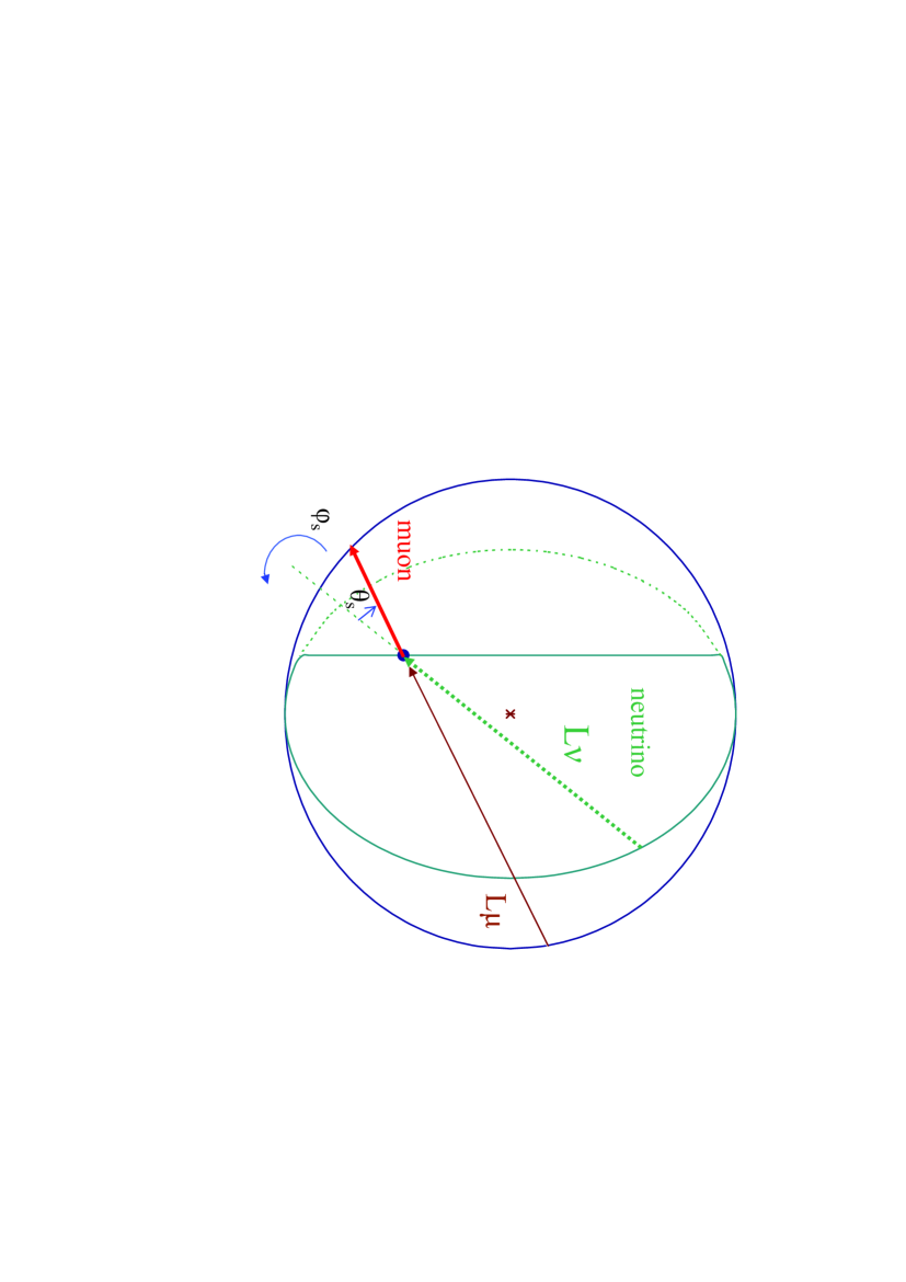
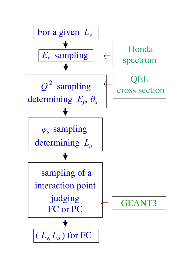
Figure 10: Schematic view of relations among $L_{\nu}$, $L_{\mu}$, $\theta_{s}$ and $\phi_{s}$ .

Figure 11: The procedure for our numerical experiment for obtaining $L_{\mu}$ from a given $L_{\nu}$.

In section 3.1 we give the procedure how to obtain $L_{\mu}$ from a neutrino event with given $L_{\nu}$ in the stochastic manner. In section 3.2 we give the correlations between $L_{\nu}$ and $L_{\mu}$, taking account of the effect of the backscattering as well as the effect of the azimuthal angle in the QEL in stochastic manner. As the result of it, we show that $L_{\nu}\approx L_{\mu}$, namely the SK assumption on the direction, does not hold even if statistically in both the absence and the presence of neutrino oscillation (Figure 13 and Figure 13). Also, we treat the correlation between $E_{\nu}$ and $E_{\mu}$, in the stochastic manner. We show that the approximation of $E_{\nu}$ with $E_{\mu}$ by Super-Kamiokande Collaboration does not make so serious error compared with the approximation of $L_{\nu}$ by $L_{\mu}$, although their treatment is theoretically unsuitable (Figure 6).

In section 4, we show that $L_{\nu}/E_{\nu}$ distribution can reproduce the minimum extrema for neutrino oscillation which SK’s neutrino oscillation parameters demand and ,furthermore, it may give the differnt mimimum extrema in the neutrino oscillation under the different neutrino oscillation parameters from SK’s. We show $L_{\nu}/E_{\nu}$ distribution can reproduce the minimum extrema for neutrino oscillation (the maximum oscillation) which Super-Kamiokande Collaboration demand, by using their neutrino oscillation parameters ($\Delta m^{2}=2.4\times 10^{-3}\rm{eV^{2}}$ and $sin^{2}2\theta=1.0$). Furthermore, it may give the different minimum extrema in the neutrino oscillation under the different neutrino oscillation parameters from the Super-Kamiokande Collaboration. This fact denotes that our numerical computer experiment is done in a correct manner.

3.1 Derivation of $L_{\mu}$ from a given $L_{\nu}$ in the single ring muon event among Fully Contained Events

In our numerical computer experiment, we obtain single ring muon events among the Fully Contained Events resulting from QEL in the virtual SK detector, the details of which are described in Appendix A. For the neutrino event with a definite neutrino energy thus generated, we simulate its interaction point inside the detector and the emitted energy of the muon concerned which gives its scattering angle uniquely. The determination of the neutrino energy, the emitted energy of the muon and its scattering angle are described in Appendix A. The muon thus generated is pursued in the stochastic manner by using GEANT 3 and finally we judge whether the muon concerned stops inside the detector (the Fully Contained Event) or passes through the detector (the Partially Contained Event). For Fully Contained Events thus obtained, we know the directions of the incident neutrinos, the generation points and termination points of the events generated inside the detector, the emitted muon energies, their scattering angles and their azimuthal angles in QEL which give their zenith angles, $L_{\nu}$ and $L_{\mu}$ finally.

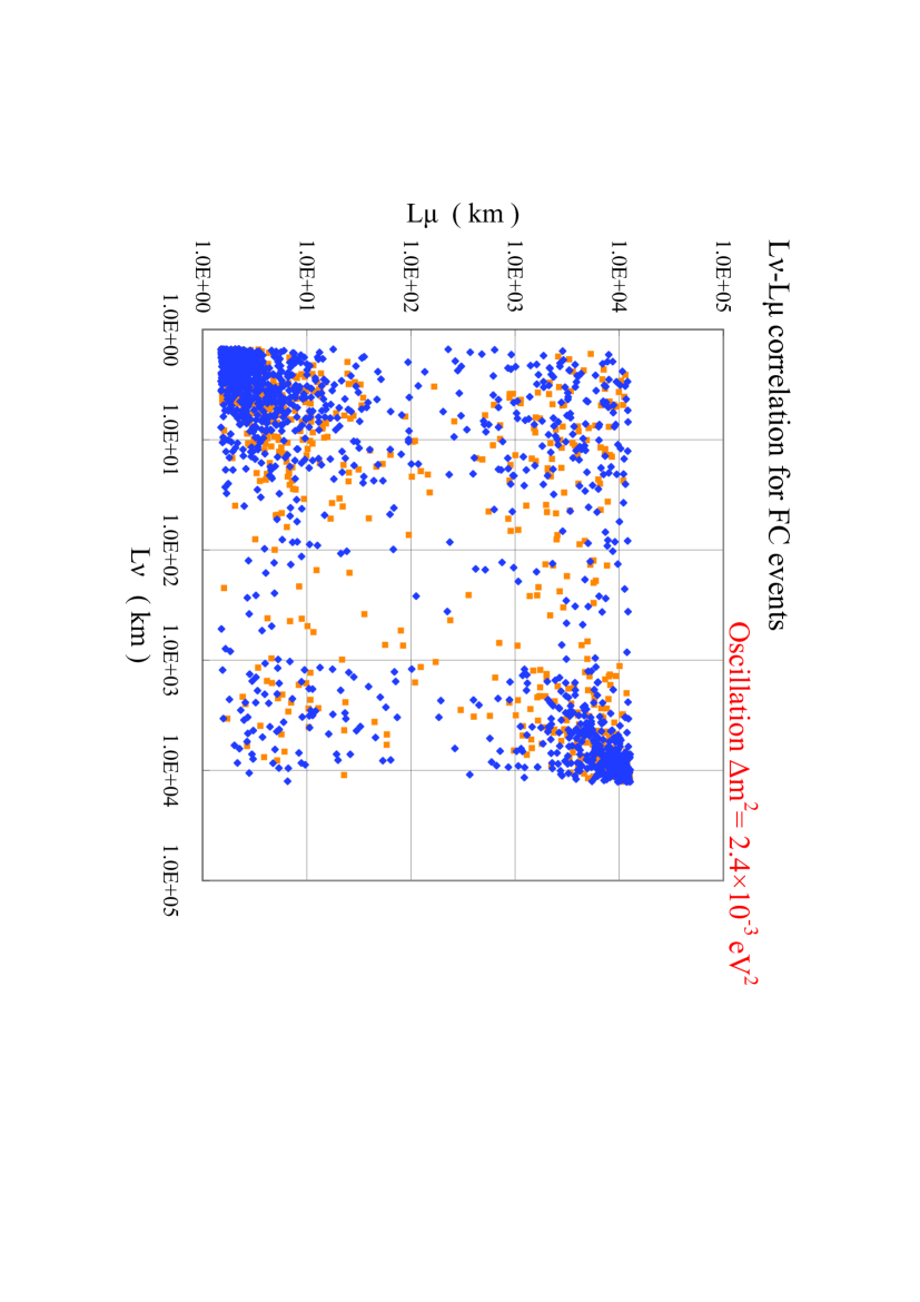
Figure 12: Correlation diagram for $L_{\nu}$ and $L_{\mu}$ without oscillation for 1489.2 live days. The blue points and orange points denote neutrino events and ani-neutrino events, respectively.

Figure 13: Correlation diagram for $L_{\nu}$ and $L_{\mu}$ with oscillation for 1489.2 live days. The blue points and orange points denote neutrino events and ani-neutrino events, respectively.

In Figure 11, we show the relation between $L_{\nu}$ and $L_{\mu}$ schematically. Figure 11 shows the procedure for obtaining $L_{\mu}$ from $L_{\nu}$ which is equivalent to the corresponding procedure for obtaining $cos\theta_{\mu}$ from $cos\theta_{\nu}$.

The relation between direction cosine of the incident neutrino, $(\ell_{\nu(\bar{\nu})},m_{\nu(\bar{\nu})},n_{\nu(\bar{\nu})})$, and that of the corresponding emitted lepton, $(\ell_{\rm r},m_{\rm r},n_{\rm r})$, for a given scattering angle, $\theta_{\rm s}$, and its azimuthal angle, $\phi$, resulting from QEL is given in Appendix A.

$L_{\nu}$ and $L_{\mu}$ are functions of the direction cosine of the incident neutrino, $cos\theta_{\nu}$, and that of emitted muon, $cos\theta_{\mu}$, respectively and they are given as,

$$L_{\nu}=R_{g}\times(r_{SK}cos\theta_{\nu}+\sqrt{r_{SK}^{2}cos^{2}\theta_{\nu}+1-r_{SK}^{2}})\,\,\,\,(5-1)$$

$$L_{\mu}=R_{g}\times(r_{SK}cos\theta_{\mu}+\sqrt{r_{SK}^{2}cos^{2}\theta_{\mu}+1-r_{SK}^{2}})\,\,\,\,(5-2)$$

where $R_{g}$ is the radius of the Earth and $r_{SK}=1-D_{SK}/R_{g}$, with the depth, $D_{SK}$, of the Super-Kamiokande Experiment detector from the surface of the Earth. It should be noticed that the $L_{\nu}$ and $L_{\mu}$ are regulated by both the energy spectrum of the incident neutrino and the production spectrum of the muon (QEL in the present case). Consequently, their mutual relation is influenced by either the absence of the oscillation or the presence of the oscillation which depend on the combination of the oscillation parameters.

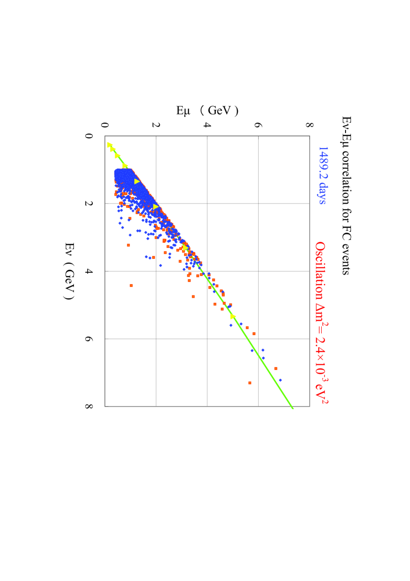
Figure 14: The correlation diagram between $E_{\nu}$ and $E_{\mu}$ for oscillation for 1489.2 live days. The continous line denotes the polynomial expression by Super-Kamiokande Collabolation.

3.2 The correlation between $L_{\nu}$ and $L_{\mu}$

In Figure 13, we give the correlation diagram between $L_{\nu}$ and $L_{\mu}$ for single ring muon events among Fully Contained Events for the 1489.2 live days in the absence of neutrino oscillation which corresponds to the actual Super-Kamiokande ExperimentAshie2 . In Figure 13, blue points denote neutrino events while orange points denote anti-
neutrino events. Throughout all correlation diagrams in the present paper, blue points and orange ones have the same meaning shown in Figure 13. The aggregates of the (anti-) neutrino events which correspond to a definite combination of $L_{\nu}$ and $L_{\mu}$ are essentially classified into four groups in the following:

Group A is defined as the aggregate for neutrino events in which both $L_{\nu}$ and $L_{\mu}$ are rather small. It denotes that the downward neutrinos produce the downward muons with smaller scattering angles. In this case, the energies of the produced muons are near the energies of the incident neutrinos due to smaller scattering angles.

Group B is defined as the aggregate for neutrino events in which both $L_{\nu}$ and $L_{\mu}$ are rather large. It denotes that the upward neutrinos produce upward muons with smaller scattering angles. In this case, the energy relation between the incident neutrinos and the produced muons is essentially the same as in Group A, because the flux of the upward neutrino events is symmetrical to that of the downward neutrino events in the absence of neutrino oscillation.

Group C is defined as the aggregate for neutrino events in which $L_{\nu}$ are rather small and $L_{\mu}$ are rather large. It denotes that the downward neutrinos produce the upward muons by the possible effect reusulting from both backscattering and azimuthal angle in QEL. In this case, the energies of the produced muons are smaller than those of the energies of the incident neutrinos due to larger scattering angles.

Group D is defined as the aggregate for the neutrino events in which $L_{\nu}$ are rather large and $L_{\mu}$ are rather small. It denotes that the upward neutrinos produce the downward muons. The energy relation between the incident neutrinos and the produced muons is essentially the same as in Group C in the absence of neutrino oscillation.

It is clear from Figure 13 that there exist the symmetries between Group A and Group B, and also between Group C and Group D, which reflect the symmetry between the upward neutrino flux and the downward neutrino one for null oscillation.

In Figure 13, we give the correlation between $L_{\nu}$ and $L_{\mu}$ under their neutrino oscillation parameters, say, $\Delta m^{2}=2.4\times 10^{-3}\rm{eV^{2}}$ and $sin^{2}2\theta=1.0$ Ashie2 . In the presence of neutrino oscillation, the property of the symmetry which holds in the absence of neutrino oscillation (see $\langle$Group A and Group B$\rangle$ and/or $\langle$Group C and Group D$\rangle$ in Figure 13) is lost due to the different incident neutrino fluxes in the upward direction and downward one. If we compare Group A with Group B, the event number in Group B (upward $\nu$ $\rightarrow$ upward $\mu$) is smaller than that in group A (downward $\nu$ $\rightarrow$ downward $\mu$), which comes from smaller flux of the upward neutrinos. The similar relation between Group C (downward $\nu$ $\rightarrow$ upward $\mu$ ) and Group D (upward $\nu$ $\rightarrow$ downward $\mu$) is held in Figure 13.

Summarizing the characteristics among Groups A to D in the Figures 13 and 13, we could conclude that $\langle$Group A and Group B$\rangle$ and $\langle$Group C and Group D$\rangle$ are in symmetrical situations in the absence of neutrino oscillation, while such a symmetrical situation is lost in the presence of neutrino oscillation. Also, it is clear from Figures 13 and 13 that $L_{\nu}\approx L_{\mu}$, namely the SK assumption on the direction, does not hold both in the absence of neutrino oscillation and in the presence of neutrino oscillation even if statistically.

Here, it should be noticed that the approximation of $L_{\nu}\approx L_{\mu}$ does not hold completely in the region C and region D. The event numbers in Group C and Group D could not be neglected among the total event number concerned. In these regions, neutrino events consist of those with backscattering and/or neutrino events in which the neutrino directions are horizontally downward (upward), but their produced muons turn upward (downward) resulting from the effect of azimuthal angles in QEL.

3.3 The correlation between $E_{\nu}$ and $E_{\mu}$

Super-Kamiokande Collaboration estimate $E_{\nu}$ from $E_{\mu}$, the visible energy of the muon, from their Monte Carlo simulation, by the following equationIshitsuka (see page 135 of the paper concerned) :

$$E_{\nu,SK}=E_{\mu}\times(a+b\times x+c\times x^{2}+d\times x^{3}),\,\,\,(6)$$

where $x=log_{10}(E_{\mu})$.

The idea that $E_{\nu}$ could be approximated as the polynomial means that there is unique relation between $E_{\nu}$ and $E_{\mu}$. However, in the light of stochastic characters inherent in both the incident neutrino energy spectrum and the production spectrum of the muon, such a treatment is not suitable theoretically, which may kill a real correlation effect between the incident neutrino energy and the emitted muon energy. In Figure 14, we give the correlation between $E_{\nu}$ and $E_{\mu}$ together with that obtained from the polynomial expression by Super-Kamiokande Collaboration under their neutrino oscillation parameters and their incident neutrino energy spectrumHonda . It is clear from the figure that the part of the lower energy incident neutrino deviates largely from the approximated formula, which reflects explicitly the stochastic character of QEL. We can give the similar relation for null oscillation, the shape of which may be different from that with oscillation due to the difference in the incident neutrino energy spectrum.

Thus, we could choose four combinations, namely $L_{\nu}/E_{\nu}$, $L_{\mu}/E_{\mu}$, $L_{\mu}/E_{\nu}$ and $L_{\nu}/E_{\mu}$ for the examination of maximum oscillations due to neutrino oscillation in $L/E$ analysis. However, only the combination of $L_{\mu}/E_{\mu}$ out of these four combinations can be physically measurable.

4 Summary

Since one cannot measure $L_{\nu}$ and $E_{\nu}$, so one is forced to utilize $L_{\mu}$ and $E_{\mu}$ in the $L/E$ analysis in place of them. Then, Super-Kamiokande Collaboration assume that the direction of the incident neutrino is the same as that of the emitted lepton the SK assumption on the direction and $E_{\nu}$ can be estimated from the some polynomial formula of the variable $E_{\mu}$ in $L/E$ analysis. However, it is clear from Figures 12 and 13 that the SK assumption on the direction does not hold even approximately and the transformation of $E_{\mu}$ into $E_{\nu}$ is not uniquely.

In the Part 2 of the subsequent paper, we apply the results from Figures 12, 13 and 14 to $L/E$ analysis and conclude that one cannot obtain the maximum oscillation in $L/E$ analysis which shows strongly the oscillation pattern from the neutrino oscillation.

APPENDIX

Appendix A Monte Carlo Procedure for the Decision of Emitted Energies of the Leptons and Their Direction Cosines

Here, we give the Monte Carlo Simulation procedure for obtaining the energy and its direction cosines, $(l_{r},m_{r},n_{r})$, of the emitted lepton in QEL for a given energy and its direction cosines, $(l,m,n)$, of the incident neutrino.

The relation among $Q^{2}$, $E_{\nu(\bar{\nu})}$, the energy of the incident neutrino, $E_{\ell(\bar{\ell})}$, the energy of the emitted lepton (muon or electron or their anti-particles) and $\theta_{\rm s}$, the scattering angle of the emitted lepton, is given as

$$Q^{2}=2E_{\nu(\bar{\nu})}E_{\ell(\bar{\ell})}(1-{\rm cos}\theta_{\rm s}).$$ (A·1)

Also, the energy of the emitted lepton is given by

$$E_{\ell(\bar{\ell})}=E_{\nu(\bar{\nu})}-\frac{Q^{2}}{2M}.$$ (A·2)

Procedure 1
We decide $Q^{2}$ from the probability function for the differential cross section with a given $E_{\nu(\bar{\nu})}$ (Eq. (2) in the text) by using the uniform random number, ${\xi}$, between (0,1) in the following

$$\xi=\int_{Q_{\rm min}^{2}}^{Q^{2}}P_{\ell(\bar{\ell})}(E_{\nu(\bar{\nu})},Q^{2}){\rm d}Q^{2},$$ (A·3)

where

$$P_{\ell(\bar{\ell})}(E_{\nu(\bar{\nu})},Q^{2})=$$

$$\frac{{\rm d}\sigma_{\ell(\bar{\ell})}(E_{\nu(\bar{\nu})},Q^{2})}{{\rm d}Q^{2}}\Bigg{/}\!\!\!\!\int_{Q_{\rm min}^{2}}^{Q_{\rm max}^{2}}\frac{{\rm d}\sigma_{\ell(\bar{\ell})}(E_{\nu(\bar{\nu})},Q^{2})}{{\rm d}Q^{2}}{\rm d}Q^{2}.$$

From Eq. (A$\cdot$1), we obtain $Q^{2}$ in histograms together with the corresponding theoretical curve in Figure 15. The agreement between the sampling data and the theoretical curve is excellent, which shows the validity of the utlized procedure in Eq. (A$\cdot$3) is right.

Figure 15: The reappearance of the probability function for QEL cross section. Histograms are sampling results, while the curves concerned are theoretical ones for given incident energies.

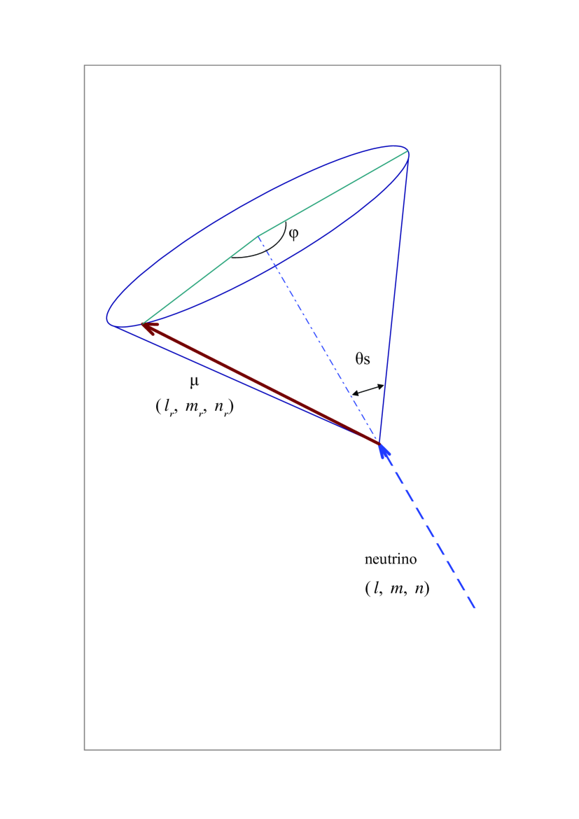
Figure 16: The relation between the direction cosine of the incident neutrino and that of the emitted charged lepton.

Procedure 2
We obtain $E_{\ell(\bar{\ell})}$ from Eq. (A$\cdot$2) for the given $E_{\nu(\bar{\nu})}$ and $Q^{2}$ thus decided in the Procedure 1.

Procedure 3
We obtain $\cos{\theta_{\rm s}}$, cosine of the the scattering angle of the emitted lepton, for $E_{\ell(\bar{\ell})}$ thus decided in the Procedure 2 from Eq. (A$\cdot$1) .

Procedure 4
We decide $\phi$, the azimuthal angle of the scattering lepton, which is obtained from

$$\phi=2\pi\xi.$$ (A·5)

Here, $\xi$ is a uniform random number between (0, 1).
As explained schematically in the text(see Figure 3 in the text), we must take account of the effect due to the azimuthal angle $\phi$ in the QEL to obtain the zenith angle distribution both for Fully Contained Events and Partially Contained Events correctly.

Procedure 5
The relation between direction cosines of the incident neutrinos, $(\ell_{\nu(\bar{\nu})},m_{\nu(\bar{\nu})},n_{\nu(\bar{\nu})})$, and those of the corresponding emitted lepton, $(\ell_{\rm r},m_{\rm r},n_{\rm r})$, for a certain $\theta_{\rm s}$ and $\phi$ is given as

$$\left(\begin{array}[]{c}\ell_{\rm r}\\ m_{\rm r}\\ n_{\rm r}\end{array}\right)=\left(\begin{array}[]{ccc}\displaystyle\frac{\ell n}{\sqrt{\ell^{2}+m^{2}}}&-\displaystyle\frac{m}{\sqrt{\ell^{2}+m^{2}}}&\ell_{\nu(\bar{\nu})}\\ \displaystyle\frac{mn}{\sqrt{\ell^{2}+m^{2}}}&\displaystyle\frac{\ell}{\sqrt{\ell^{2}+m^{2}}}&m_{\nu(\bar{\nu})}\\ -\sqrt{\ell^{2}+m^{2}}&0&n_{\nu(\bar{\nu})}\end{array}\right)\left(\begin{array}[]{c}{\rm sin}\theta_{\rm s}{\rm cos}\phi\\ {\rm sin}\theta_{\rm s}{\rm sin}\phi\\ {\rm cos}\theta_{\rm s}\end{array}\right),$$ (A·6)

where $n_{\nu(\bar{\nu})}={\rm cos}\theta_{\nu(\bar{\nu})}$, and $n_{\rm r}={\rm cos}\theta_{\ell}$. Here, $\theta_{\ell}$ is the zenith angle of the emitted lepton.

The Monte Carlo procedure for the determination of $\theta_{\ell}$ of the emitted lepton for the parent (anti-)neutrino with given $\theta_{\nu(\bar{\nu})}$ and $E_{\nu(\bar{\nu})}$ involves the following steps:

We obtain $(\ell_{r},m_{r},n_{r})$ by using Eq. (A·6). The $n_{r}$ is the cosine of the zenith angle of the emitted lepton which should be contrasted to $n_{\nu}$, that of the incident neutrino.
Repeating the procedures 1 to 5 just mentioned above, we obtain the zenith angle distribution of the emitted leptons for a given zenth angle of the incident neutrino with a definite energy.

In the SK analysis, instead of Eq. (A·6), they assume
$n_{r}=n_{\nu(\bar{\nu})}$ uniquely for ${E_{\mu(\bar{\mu})}}\geq$ 400 MeV.

References

-
(1)
Hirata, KS et al., Phys.Lett.B205(1988)416.
Hirata, KS et al., Phys.Lett.B280(1992)146.
Casper, D et al., Phys.Rev.Lett.66(1991)2561.
Becker-Szendy, R et al., Phys.Rev. D 46(1992)3720. - (2) Hatakeyama, S et al., Phys.Rev.Lett.81(1998)2010.
-
(3)
Kajita, T,
Neutrino 98, Takayama, Japan, June 4-9 19982.
Fukuda, Y, Phys.Rev.Lett.81(1998)1562. -
(4)
Mann, WA, Nucl.Phys.Proc.Supple Vol.91(2000)134.
Ambrosio, Met al., Phys.Lett.B478(2000)3. - (5) K2K, Phys.Rev. D74(2006)72003.
- (6) Michael, DG et al., Phys.Rev.Lett.97(2006) 191801.
- (7) Ashie,Y. et al., Phys. Rev. D 71 (2005) 112005.
- (8) Kajita, T. and Totsuka, Y. Rev. Mod. Phys., 73 (2001)85. See p.101.
- (9) Ishitsuka, M, Ph.D thesis, University of Tokyo (2004). See p. 138.
- (10) Jung, CK, Kajita, T, Mann, T and McGrew, C, Anual. Rev. Mod. Sci. vol.15 (2005) 431.
- (11) Renton, P., Electro-weak Interaction, Cambridge University Press (1990). See p. 405.
-
(12)
Honda, M., et al., Phys. Rev. D 52 (1996) 4985.
Honda, M., et al., Phys. Rev. D 70 (2004)043008-1. - (13) Ashie,Y et al., Phys.Rev.Lett.93 (2004)101801-1.