Gaussian integration with rescaling of abscissas and weights

Abstract

An algorithm for integration of polynomial functions with variable weight is considered. It provides extension of the Gaussian integration, with appropriate scaling of the abscissas and weights. Method is a good alternative to usually adopted interval splitting.

1 Introduction : the integral

In many areas of the physics and chemistry, the following integral emerges:

$$I(a)=\int_{1}^{\infty}\frac{g(x)}{1+e^{x/a}}\;dx$$ (1)

where $g(x)$ is a smooth function and $0<a<\infty$ a real parameter. Here we assume that function $g(x)$ can be successfully approximated by the polynomial. For a fixed value of $a$ the standard method for numerical evaluation of such an integral is Gaussian integration or similar closely related algorithm.

The difficulties caused by the integral of the form (1) can be show by comparison with other similar examples. If we change lower integration limit from 1 to zero, one can easily remove parameter $a$ from the algorithm by the substitution $x=at$:

$$a\int_{0}^{\infty}\frac{g(at)}{1+e^{t}}\;dt.$$

Parameter $a$ now appear in the function $g$, and modified (because of 1 in the denominator) Gauss-Laguerre algorithm can be used.

Similarly, if we remove 1 from the denominator, the substitution $z=(x-1)/a$ transform integral into form:

$$ae^{-1/a}\int_{0}^{\infty}g(1+az)e^{-z}\;dz$$

easily integrable numerically with standard Gauss-Laguerre algorithm.

However, when both the lower integration limit is 1, and 1 is present in the denominator, parameter $a$ cannot be eliminated from Eq. (1): it always appears either outside function $g$ in non-linear way, or enters the limit(s) of integration. This does not prevent us from calculating abscissas and weights of the Gauss-like quadrature for any fixed value of $a$, say $a=1$, $a=3$ or $a=1/4$. The general idea of the algorithm presented in this article, is to use Gauss-like quadrature with abscissas and weights being functions of parameter $a$.

Standard method to handle integrals of the form (1) is to split integration interval into at least two: $1\leq x<\xi$, $\xi\leq x<\infty$. If the value of $\xi$ is chosen properly as a function of $a$, then in the first interval we have:

$$\frac{1}{1+e^{x/a}}\sim\frac{1}{e^{\frac{1}{a}}+1}-\frac{e^{\frac{1}{a}}(x-1)}{a\left(e^{\frac{1}{a}}+1\right)^{2}}+O\left((x-1)^{2}\right),$$

that is, weight is nearly linear (or polynomial if using higher order expansion). In this interval we can use Gauss-Legendre integration. For $x>\xi$, 1 in the denominator can be omitted, and Gauss-Laguerre quadrature apply. In practice, more interval subdivisions are required [1, 2, 3].

2 Case with fixed parameter

We start analysis with simplest case of $a=1$ in Eq. (1). The integral becomes:

$$I(1)=\int_{1}^{\infty}\frac{g(x)}{1+e^{x}}\;dx$$ (2)

For $g(x)=x^{n}$, where $n$ is non-negative integer, we have found that moments are equal to:

$$M(n,1)\equiv\int_{1}^{\infty}\frac{x^{n}}{1+e^{x}}\;dx=-\sum_{k=1}^{n+1}\left(\prod_{i=1}^{k-1}n+i-k+1\right)\mathrm{Li}_{k}\left(-\frac{1}{e}\right)$$ (3)

where $\mathrm{Li}_{k}$ is the polylogarithm. Our goal is to find weights, $W_{i}$, and abscissas, $X_{i}$, of the Gaussian quadrature formula:

$$\int_{1}^{\infty}\frac{P_{n}}{1+e^{x}}\;dx=\sum_{i=1}^{N_{gauss}}W_{i}P_{n}(X_{i}),$$ (4)

where $P_{n}$ is polynomial of the order up to $2N_{gauss}-1$.

Convenient method [4] to find weights and Gauss points uses orthogonal polynomials $Q_{n}$ related to given weight:

$$\int_{1}^{\infty}\frac{Q_{n}Q_{m}}{1+e^{x}}\;dx=\delta_{nm}.$$

Unfortunately, as noted by [5], for infinite integration interval calculations still require arbitrary precision calculations. Problem is increasingly ill-conditioned numerically. We have found, that the best method is to solve system of equations for unknown polynomial coefficients in eq. (4) progressively. We use already found coefficients for polynomials of the order $n-1$, and Laguerre polynomial $L_{n}$ coefficients as a guess starting points. System of the equations is then solved numerically using arbitrary precision arithmetic. Results were verified using method of [6].

Once orthogonal polynomials are found, abscissas are zeros of the $Q_{n}$, and weights are equal to [5]:

$$W_{i}=\left(\sum_{k=1}^{n-1}Q_{k}(X_{i})^{2}\right)^{-1}.$$

Another equivalent formula for weights is [4]:

$$W_{i}=-\frac{k_{n}}{k_{n-1}}\left(Q_{n}(X_{i})Q_{n-1}^{{}^{\prime}}(X_{i})\right)^{-1}$$

Knowledge of abscissas and weights for integral with $a=1$ is crucial, because of the approximate scaling found and used in the next section to derive more general results for $a\neq 1$.

3 Scaling of abscissas and weights

For integral (1) with function $g(x)$ being equal to $x^{n}$ we can provide formula similar to (3), generalized to case $a\neq 1$:

$$M(n,a)=\int_{1}^{\infty}\frac{x^{n}}{1+e^{x/a}}\;dx=-\sum_{k=1}^{n+1}a^{k}\,\left(\prod_{i=1}^{k-1}n+i-k+1\right)\mathrm{Li}_{k}\left(-\frac{1}{e^{1/a}}\right)$$ (5)

Knowledge of the moments facilitates calculations of abscissas and weights, but in practice polylogarithms present in eq. (5) often is not directly available. One must calculate moments by means of direct numerical integration. In principle, using (5), one can find orthogonal polynomials (and Gaussian quadrature abscissas and weights as well) analytically. However, formulae become ridiculously complicated already for $n>2$, and we restrict discussion to case of $n=1$.

Unfortunately, we were unable to derive general formulae for orthogonal polynomials $Q_{n}$ or find coefficients of the three-term recurrence formula.

3.1 Single Gaussian point quadrature

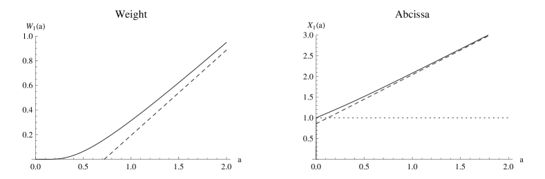
Figure 1: Weight (left) and abscissa (right) and for single point Gaussian quadrature as a functions of $a$, and its asymptotes (dashed).

While the case of single Gaussian point is not interesting from practical point of view, it gives some insights into planned procedure due to very simple formulae. Quadrature is:

$$\int_{1}^{\infty}\frac{g(x)}{1+e^{x/a}}\;dx\simeq w_{1}g(x_{1}),$$ (6)

where:

$$w_{1}=a\ln{(1+e^{-1/a})}\equiv a\;\mathrm{Li}_{1}(-e^{-1/a}),\quad x_{1}=1+a\;\frac{\mathrm{Li}_{2}(-e^{-1/a})}{\mathrm{Li}_{1}(-e^{-1/a})}$$ (7)

Integration algorithm based on abscissa and weight provided above is exact only for constant functions. Weight and abscissa are shown in Fig. 1. Functions $\mathrm{Li}_{k}(-e^{-1/a})$ present in the formulas above are somewhat pathological. All derivatives vanish at $a=0$:

$$\lim_{a\to 0^{+}}\frac{d^{n}}{da^{n}}\mathrm{Li}_{k}(-e^{-1/a})=0.$$

Therefore, the function $\psi(a)$ defined as follows:

$$\psi(a)=\begin{cases}0&a\leq 0\\ \mathrm{Li}_{k}(-e^{-1/a})&a>0\end{cases}$$ (8)

is an example of the infinitely differentiable function which is non-analytic at $a=0$. Therefore, it cannot be approximated by the polynomials near $a=0$. For $a\to\infty$ we have:

$$\lim_{a\to\infty}\mathrm{Li}_{k}(-e^{-1/a})=\begin{cases}-\ln{2}&\quad k=1\\ \left(4^{(1-k)/2}-1\right)\,\zeta(k)&\quad k>1\end{cases}$$ (9)

where $\zeta$ is Riemann-zeta function. Both functions $W_{1}(a)$ and $X_{1}(a)$ approach their asymptotes very slowly, cf. Fig. 1.

3.2 General Gaussian quadrature

For $a\neq 1$, due to extremely complicated formulae, discussion will be limited to numerical results. It is observed, that functions $W_{i}(a)$ and $X_{i}(a)$ behave like functions $W_{1}(a)$ and $X_{1}(a)$ discussed in previous subsection. Rough approximation for abscissas and weights (arbitrary order) can be combined from results for $a=1$, and single point quadrature as follows:

$$X_{i}(a)\simeq 1+a\,\lambda_{i},\qquad W_{i}(a)\simeq\delta_{i}\,(-1+a\ln{(1+e^{1/a})})$$ (10)

where $\lambda_{i}=1+X_{i}(1)$ and $\delta_{i}=W_{i}(1)/(-1+\ln{(1+e)})$. Values of $W_{i}(1)$ and $X_{i}(1)$ are simply weights and abscissas for $a=1$ quadrature, cf. Sect. 2.

Example results are presented in Fig. 2 using lines. Gauss points behave as expected for $a\to 0$, that is, they concentrate near $x=1$. For $a\to\infty$ abscissas spread from $x=1$ to infinity. Weight also behave correctly, scaling linearly with $a\to\infty$ and approaching zero as $a\to 0$. For $a\to 0$, formulae (10) are progressively better approximations. Note however, that (10) do not provide correct asymptotic behavior for $a\to\infty$. This would require knowledge of analytical formulae for $W_{i}(a)$ and $X_{i}(a)$, or its asymptotic expansion at least.

Parameterization (10) provides excellent starting guess points for numerical calculations of $W_{i}(a)$ and $X_{i}(a)$.

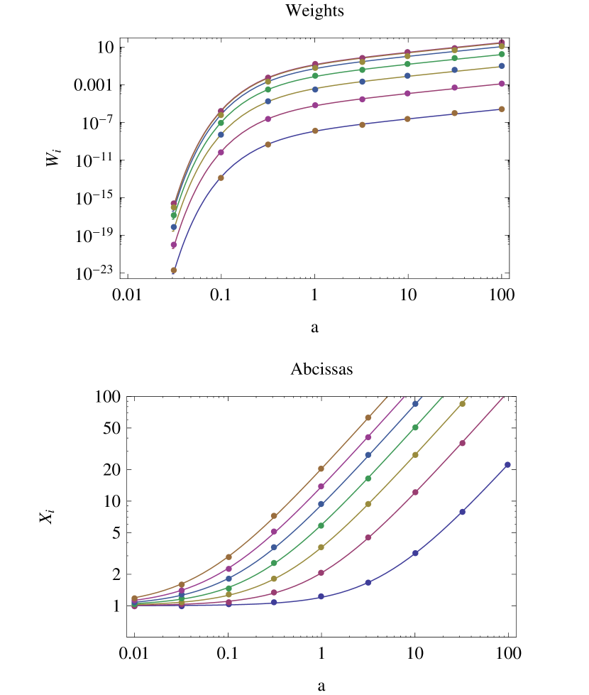
Figure 2: Numerically obtained Gaussian weights and abscissas for integral of the form (1) (points) compared to formulae (10) (lines). 7-point quadrature is shown.

Typical numerical result is shown in Fig. 2 using bullets. Apparent accuracy of the scaling (10) is misleading, because (i) logarithmic scale hide errors (ii) very high accuracy is required for Gaussian quadrature to work. Therefore quadrature obtained from (10) is not expected to be very accurate, except maybe for $a\ll 1$. Nevertheless, overall picture is appealing, and use of scaling, possibly not as simple as (10), seems to be move in the promising direction. At present, however, we are forced to use interpolation of numerically computed values. For values of $a$ outside interpolation domain we can use asymptotes for $a\gg 1$, and (8) for $a\ll 1$.

4 Performance of the algorithm

Approximate value of the integral (1) is computed from formula:

$$I(a)\simeq\sum_{i=1}^{N_{gauss}}W_{i}(a)P_{n}\left(X_{i}(a)\right)$$ (11)

where, in contrast to (4), $W_{i}$ and $X_{i}$ are functions of $a$, cf. Fig. 2.

There are two factors determining accuracy of the method: number of Gaussian points, $N_{gauss}$, and accuracy of the functions $W_{i}(a),X_{i}(a)$, $i=1\ldots N_{gauss}$. The latter depends on number of sampling points, $N_{sampl}$, and algorithm used to interpolate between them. Ideally, we would like to have many Gauss points, and very accurate (or exact) scaling of them. In practice we should know what is better: large $N_{gauss}$ with small $N_{sampl}$, or vice versa. We address these questions in next subsections.

4.1 Accuracy as a function of Gaussian points $N_{gauss}$

In this subsection we keep number of sampling points used to interpolate functions $W_{i}(a)$ and $X_{i}(a)$ fixed. Number of these functions will be varied. Naively, from definition of the Riemann integral, we expect that more sampling points could result in increased accuracy regardless of the algorithm used, as long as integral is convergent. On the other hand Gaussian quadrature of polynomials is exact up to certain order, but only for precisely determined abscissas and weights. Algorithm is then expected to fail (in the sense of accuracy) for polynomials except at the grid points. For non-polynomial functions Gaussian integration is only approximate functional, and accuracy of $W_{i},X_{i}$ is possibly less important.

Now we attempt to test these expectations using two examples of interest:

$$g_{1}(x)=x+x^{4}-x^{5},\qquad\text{polynomial exactly integrable}$$ (12a)

$$g_{2}(x)=x^{4}\sqrt{1+x},\qquad\text{function arising from relativistic momentum}$$ (12b)

Number of sampling points has been fixed to 50 per decade per function. In the range of $0.01\leq a\leq 100$ total of 201 points spaced logarithmically were used. Third and eight order interpolation were used for abscissas and weights, respectively.

Figure 3: Relative errors versus $a$ for $N_{gauss}=3$ (dotted), $5$ (dashed) and $11$ (solid) for polynomial (12a).

Three cases are compared: $N_{gauss}=3,7$ and $11$. Relative accuracy obtained for polynomial (12a) is presented in Fig. 3. Differences are barely visible, and error is entirely due to variations of the abscissas and weights. Normally, for polynomial of the order $\leq 5$ we expect to achieve relative error of the order of machine epsilon (Fig. 3, thin line near bottom; axis is placed at $\epsilon=2.2\times 10^{-16}$). Therefore, this figure shows errors caused by the interpolation of the abscissas and weights. Error estimate reach huge values for small values of $a$. However, in typical application integrals of the form (1) are calculated over wide range of parameters and summed up. Therefore overall absolute error is mainly due to regions with large $a$ where the numerical value of the integral is largest. Interpolation error visible in Fig. 3 might be significantly reduced if required, cf. Sect. 4.2 and Figs. 5, 6.

Figure 4: Like in Fig. 3, but for non-polynomial function (12b).

Test case $g_{2}$ (12b) provides more realistic task for the algorithm. This time number of Gaussian points do matter, especially for $a>1$. Thin lines show relative accuracy achieved exactly at grid points. For $a>1$, algorithm surprisingly provides accuracy nearly identical to normal Gaussian integration. It is however clear from Fig. 4, that accuracy better than $\sim 10^{-10}$ cannot be achieved, regardless of the value of $N_{gauss}$. We need more dense grid of points used to interpolate functions $W_{i}(a),X_{i}(a)$ in (11), or better interpolation algorithm, cf. Sect. 4.2. Again, for $a\ll 1$ relative accuracy is poor, but integral values are very small in this regime due to exponential factor in the integrand of (1). For small $a$ one can also consider use of (10) instead of numerical values, see Fig. 5, red line.

4.2 Accuracy as a function of sampling points $N_{sampl}$

In this subsection we keep number of Gaussian points fixed, $N_{gauss}=7$. Number of sampling points will be increased, so interpolated functions $W_{i}(a),X_{i}(a)$ will approach their exact values. For polynomials up to the order $2N_{gauss}-1=13$, integration algorithm is expected to achieve machine precision – in limiting case at least. For other functions it should be no worse than ordinary Gauss-Laguerre-like integration with fixed weight.

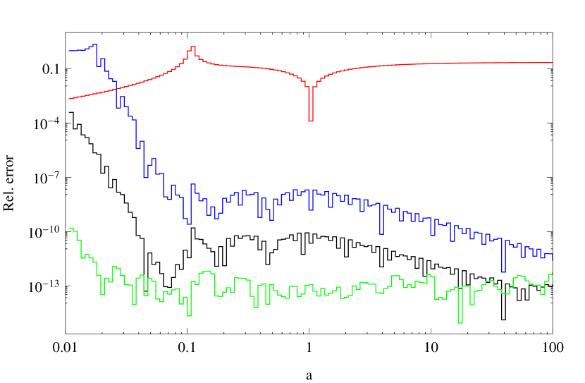
Figure 5: Relative errors versus $a$ caused in the final integral using increased number of interpolation points used to restore abscissas and weights for integrand (12a). Red - analytical formula, blue - 50/decade, black -200/decade, green - 1000/decade.

Typical result is presented in Fig. 5. Let us remind, that in the case of exact abscissas and weights for polynomial (12a) we expect to achieve machine precision. In Fig. 5 $\epsilon=2.2\times 10^{-16}$, where lower axis has been placed. Third order interpolation has been used do compute abscissas and eight order to compute weights. Analytical formula (10) is shown in red for reference. It is not surprise, that using progressively more interpolation points we get better results (Fig. 5). Using 1000 points per decade (Fig. 5, green), relative accuracy is at level of $10^{-13}$.

4.2.1 Influence of the interpolation order and method

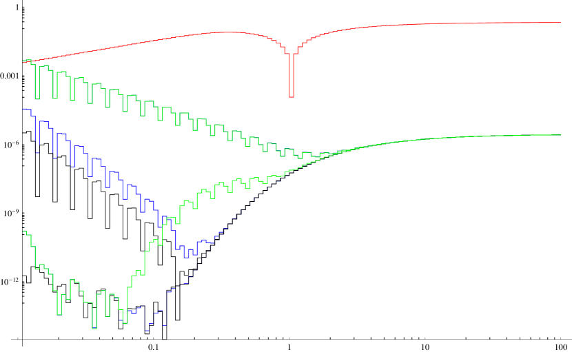
Figure 6: Relative errors versus $a$ caused in the final integral using various interpolation algorithms used to restore abscissas and weights (using 1000 points per decade) for integrand (12b). Red - analytical formula, blue - Hermite, black - splines, green - mixed orders (see text).

Interpolation goal is to reproduce abscissas and weights from discrete set of points as accurately as possible. Besides number of these points, which is obvious factor, secondary important issues are: interpolation method, interpolation order and location of the points. Influence of various factors on relative integration error in the case of function (12b) is presented in Fig. 6. 4000 points spaced logarithmically has been used in the range from 0.01 to 100, i.e. thousand points per decade. Two standard interpolation algorithms: Hermite and spline were used with order 1 (linear), 3 and 8. Noteworthy, relative error gain obtained from increase of the interpolation order from 3 to 8 is as high as six orders of magnitude. Further test has shown, that gain is almost entirely due to accuracy of weights. Abscissas are successfully approximated even using linear interpolation, cf. green lines in Fig. 6. Interpolation order and method is important mainly if $a<1$. For $a\gg 1$ no differences are visible.

Possibly, using non-linearly scattered points and renormalized function values we would be able to increase accuracy further without increasing number of points. This might be important issue in real-world implementation of the algorithm. Too large amount of data can result in cache misses of modern CPUs, slowing down calculations.

5 Concluding remarks

Novel algorithm for evaluation of the improper integrals with a real parameter (1) in the weight function has been presented. Method is based on Gaussian integration, where abscissas and weights are functions of parameter $a$ rather than just real numbers. Both analytical and numerical approximations of these functions are considered. Algorithm is shown to be robust and useful.

Presented method might be considered to be an example of rendering of the multivariate function into number of functions of one variable. The latter can be approximated very accurately, and do not consume computer memory, in contrast to tabulations of multivariate functions. Therefore the fact, that functions $W_{i}$ are not already known in terms of e.g. elementary functions is not serious limitation for modern hardware.

Possible direction of further research are: (i) search for exact scaling formulae or their approximations (ii) scaling in limiting cases $a\to 0$ and $a\to\infty$ (iii) dedicated interpolation formulae (iv) use of scaling with non-Gaussian (e.g. trapezoidal) integration rules. Properties of the related orthogonal (non-classic) polynomials are also of interest, particularly three-term recurrence formula and behavior of the leading terms.

References

- [1] Gong, Z., Zejda, L., Däppen, W., and Aparicio, J. M., Computer Physics Communications 136 (2001) 294.
- [2] Timmes, F., Cococubed.com, http://cococubed.asu.edu/code_pages/fermi_dirac.shtml, 2008.
- [3] Aparicio, J. M., Astrophysical Journal Supplement 117 (1998) 627.
- [4] Golub, G. H. and H., W. J., Mathematics of Computation 23 (1969) 221.
- [5] Gautschi, W., Mathematics of Computation 24 (1970) 245.
- [6] Fukuda, H., Katuya, M., Alt, E., and Matveenko, A., Computer Physics Communications 167 (2005) 143 .